Báo cáo hóa học: " Research Article A New Multistage Lattice Vector Quantization with Adaptive Subband Thresholding for Image Compression"

Chia sẻ: Linh Ha | Ngày: | Loại File: PDF | Số trang:11

Thêm vào BST

Báo xấu

44
lượt xem 3
download

Download Vui lòng tải xuống để xem tài liệu đầy đủ

Tuyển tập báo cáo các nghiên cứu khoa học quốc tế ngành hóa học dành cho các bạn yêu hóa học tham khảo đề tài: Research Article A New Multistage Lattice Vector Quantization with Adaptive Subband Thresholding for Image Compression

Chủ đề:

Bình luận(0) Đăng nhập để gửi bình luận!

Lưu

Nội dung Text: Báo cáo hóa học: " Research Article A New Multistage Lattice Vector Quantization with Adaptive Subband Thresholding for Image Compression"

Hindawi Publishing Corporation EURASIP Journal on Advances in Signal Processing Volume 2007, Article ID 92928, 11 pages doi:10.1155/2007/92928 Research Article A New Multistage Lattice Vector Quantization with Adaptive Subband Thresholding for Image Compression M. F. M. Salleh and J. Soraghan Institute for Signal Processing and Communications, Department of Electronic and Electrical Engineering, University of Strathclyde, Royal College Building, Glasgow G1 1XW, UK Received 22 December 2005; Revised 2 December 2006; Accepted 2 February 2007 Recommended by Liang-Gee Chen Lattice vector quantization (LVQ) reduces coding complexity and computation due to its regular structure. A new multistage LVQ (MLVQ) using an adaptive subband thresholding technique is presented and applied to image compression. The technique con- centrates on reducing the quantization error of the quantized vectors by “blowing out” the residual quantization errors with an LVQ scale factor. The signiﬁcant coeﬃcients of each subband are identiﬁed using an optimum adaptive thresholding scheme for each subband. A variable length coding procedure using Golomb codes is used to compress the codebook index which produces a very eﬃcient and fast technique for entropy coding. Experimental results using the MLVQ are shown to be signiﬁcantly better than JPEG 2000 and the recent VQ techniques for various test images. Copyright © 2007 M. F. M. Salleh and J. Soraghan. This is an open access article distributed under the Creative Commons Attribution License, which permits unrestricted use, distribution, and reproduction in any medium, provided the original work is properly cited. 1. INTRODUCTION that produced results that are comparable to JPEG 2000 [9] at low bit rates. Recently there have been signiﬁcant eﬀorts in producing ef- Image compression schemes that use plain lattice VQ have been presented in [3, 6]. In order to improve perfor- ﬁcient image coding algorithms based on the wavelet trans- mance, the concept of zerotree prediction as in EZW [10] form and vector quantization (VQ) [1–4]. In [4], a review of or SPHIT [11] is incorporated to the coding scheme as pre- some of image compression schemes that use vector quan- sented in [12]. In this work the authors introduce a technique tization and wavelet transform is given. In [1] a still image called vector-SPHIT (VSPHIT) that groups the wavelet coef- compression scheme introduces an adaptive VQ technique. The high frequency subbands coeﬃcients are coded using ﬁcients to form vectors before using zerotree prediction. In addition, the signiﬁcant coeﬃcients are quantized using the a technique called multiresolution adaptive vector quanti- voronoi lattice VQ (VLVQ) that reduces computational load. zation (MRAVQ). The VQ scheme uses the LBG algorithm Besides scanning the individual wavelet coeﬃcients based on wherein the codebook is constructed adaptively from the in- zerotree concept, scanning blocks of the wavelet coeﬃcients put data. The MRAVQ uses a bit allocation technique based has recently become popular. Such work is presented in [13] on marginal analysis, and also incorporates the human visual called the “set-partitioning embedded block” (SPECK). The system properties. MRAVQ technique has been extended to work exploits the energy cluster of a block within the sub- video coding in [5] to form the adaptive joint subband vec- band and the signiﬁcant coeﬃcients are coded using a sim- tor quantization (AJVQ). Using the LBG algorithm results in ple scalar quantization. The work in [14] uses VQ to code the high computation demands and encoding complexity partic- signiﬁcant coeﬃcients for SPECK called the vector SPECK ularly as the vector dimension and bit rate increase [6]. The lattice vector quantization (LVQ) oﬀers substantial reduction (VSPECK) which improves the performance. The image coding scheme based on the wavelet trans- in computational load and design complexity due to the lat- form and vector quantization in [1, 2] searches for the signif- tice regular structure [7]. The LVQ has been used in many icant subband coeﬃcients by comparing them to a threshold image coding applications [2, 3, 6]. In [2] a multistage resid- value at the initial compression stage. This is followed by a ual vector quantization based on [8] is used along with LVQ
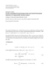
2 EURASIP Journal on Advances in Signal Processing Consider a sequence of length N having n zeros and a one quadtree modelling process of the signiﬁcant data location. {00 · · · 01} The threshold setting is an important entity in searching for the signiﬁcant vectors in the subbands. Image subbands at X = 0n 1 ; where N = n + 1. (1) diﬀerent levels of decomposition carry diﬀerent degrees of information. For general images, lower frequency subbands Let p be the probability of a zero, and 1 − p is the probability carry more signiﬁcant data than higher frequency subbands of a one [15]. Therefore there is a need to optimize the threshold P (0) = p, P (1) = 1 − p. (2) values for each subband. A second level of compression is achieved by quantizing the signiﬁcant vectors. The probability of the sequence X can be expressed as Entropy coding or lossless coding is traditionally the last P (n) = pn (1 − p). stage in an image compression scheme. The run-length cod- (3) ing technique is very popular choice for lossless coding. Ref- The optimum value of the group size b is [12] erence [16] reports an eﬃcient entropy coding technique for sequences with signiﬁcant runs of zeros. The scheme 1 b= − . (4) is used on test data compression for a system-on-a-chip log2 p design. The scheme incorporates variable run-length cod- ing and Golomb codes [17] which provide a unique binary The run-length integers are grouped together, and the ele- representation for run-length integer symbol with diﬀerent ment in the group set is based on the optimum Golomb pa- lengths. It also oﬀers a fast decoding algorithm as reported in rameter b found in (4). The run lengths (integer symbols) group set G1 is {0, 1, 2, . . . , b − 1}; the run lengths (integer [18]. symbols) group set G2 is {b, b + 1, b + 2, . . . , 2b − 1}; and so In this paper, a new technique for searching the signif- forth. If b is a value of the power of two (b = 2N ), then each icant subband coeﬃcients based on an adaptive threshold- group Gk will have 2N number of run lengths (integer sym- ing scheme is presented. A new multistage LVQ (MLVQ) bols). In general, the set of run lengths (integer symbols) Gk procedure is developed that eﬀectively reduces the quantiza- is given by the following [17]: tion errors of the quantized signiﬁcant data. This is achieved as a result of having a few quantizers in series in the en- Gk = (k − 1)b, (k − 1)b + 1, (k − 1)b + 2, . . . , kb − 1 . coding algorithm. The ﬁrst quantizer output represents the (5) quantized vectors and the remaining quantizers deal with the quantization errors. For stage 2 and above the quan- Each group of Gk will have a preﬁx and b number of tails. tization errors are “blown out” using an LVQ scale factor. The preﬁx is denoted as (k − 1)1s followed by a zero deﬁned This allows the LVQ to be used more eﬃciently. This diﬀers as from [2] wherein the quantization errors are quantized un- preﬁx = 1(k−1) 0. (6) til the residual quantization errors converge to zero. Finally the variable length coding with the Golomb codes is em- The tails is a binary representation of the modulus operation ployed for lossless compression of the lattice codebook index between the run length integer symbol and b. Let n be the data. length of tail sequence The paper is organized as follows. Section 2 gives a review n = log2 b, of Golomb coding for lossless data compression. Section 3 reviews basic vector quantization and the lattice VQ. The tail = mod(run length symbol, b) with n bits length. new multistage LVQ (MLVQ), adaptive subband threshold- (7) ing algorithm, and the index compression technique based on Golomb coding are presented in Section 4. The perfor- The codeword representation of the run length consists mance of the multiscale MLVQ algorithm for image com- of two parts, that is, the preﬁx and tail. Figure 1 summa- rized the process of Golomb coding for b = 4. From (5) pression is presented in Section 5. MLVQ is shown to be sig- the ﬁrst group will consist of the run-length {0, 1, 2, 3} or niﬁcantly superior to Man’s [2] method and JPEG 2000 [9]. G1 = {0, 1, 2, 3}, and G2 = {4, 5, 6, 7}, and so forth. Group It is also better than some recent VQ works as presented in 1 will have a preﬁx {0}, group 2 will have preﬁx {10}, and [12, 14]. Section 6 concludes the paper. so forth. Since the value of b is chosen as 4, the length of tail is log2 4 = 2. For run-length 0, the tail is represented by bits 2. GOLOMB CODING {00}, the tail for run-length 1 is represented by bits {10}, and In this section, we review the Golomb coding and its appli- so forth. Since the codeword is the combination of the group cation to binary data having long runs of zeros. The Golomb preﬁx and the tail, for run-length of 0 will have the codeword of {000} where the ﬁrst 0 is the group preﬁx and the remain- code provides a variable length code of the integer symbol [17]. It is characterized by the Golomb code parameter b ing 0 s is the tail, the run-length 1 will have codeword {001}, which refers to the group size of the code. The choice of the and so forth. Figure 1(b) shows the example of the encoding optimum value b for a certain data distribution is a non- process with 32 bits input with 6 ones (r = 6) which can be trivial task. An optimum value of b for random distribution encoded as 22 bits. The Golomb codes oﬀer an eﬃcient tech- of binary data has been found by Golomb [17] as follows. nique for run-length coding (variable-length coding).
M. F. M. Salleh and J. Soraghan 3 the codewords. The peak energy is deﬁned as the squared dis- Group Run length Group preﬁx Tail Codeword tance of an output point (lattice point) farthest from the ori- 0 00 000 gin. This rule dictates the ﬁlling order of L codewords start- 1 01 001 G1 0 ing from the innermost shells. The number of lattice point on 2 10 010 each shell is obtained from the coeﬃcient of the theta func- 3 11 011 tion [7, 20]. Sloane has tabulated the number of lattice points 4 00 1000 in the innermost shells of several root lattices and their dual 5 01 1001 [21]. G2 10 6 10 1010 7 11 1011 3.2. Lattice type 8 00 11000 A lattice is a regular arrangement of points in k-space that 9 01 11001 G3 110 includes the origin or the zero vector. A lattice is deﬁned as a 10 10 11010 set of linearly independent vectors [7]; 11 11 11011 ··· ··· ··· ··· ··· Λ = X : X = a1 u1 + a2 u2 + · · · + aN uN , (9) (a) Golomb coding for b = 4 where Λ ∈ k , n ≤ k, ai and ui are integers for i = 1, 2, . . . , N . The vector set {ui } is called the basis vectors of S = {000001 00001 00000001 1 00000001} lattice Λ, and it is convenient to express them as a generating matrix U = [u1 , u2 , . . . , un ]. l1 = 5 l2 = 4 l3 = l5 = 0 l6 = 7 The Z n or cubic lattice is the simplest form of a lattice structure. It consists of all the points in the coordinate sys- tem with a certain lattice dimension. Other lattices such as CS = {1001 1011} 1000 1011 000 Dn (n ≥ 2), An (n ≥ 1), En [n = 6, 7, 8], and their dual are (b) Example of encoding using the Golomb the densest known sphere packing and covering in dimen- code b = 4, CS = 19 bits sion n ≤ 8 [16]. Thus, they can be used for an eﬃcient lattice vector quantizer. The Dn lattice is deﬁned by the following Figure 1 [7]: n Dn = x 1 , x 2 , . . . , x n ∈ Z n , xi = even. 3. VECTOR QUANTIZATION where (10) i=1 3.1. Lattice vector quantization The An lattice for n ≥ 1 consists of the points of (x0 , x1 , . . . , xn ) with the integer coordinates sum to zero. The Vector quantizers (VQ) maps a cluster of vectors to a sin- lattice quantization for An is done in n + 1 dimensions and gle vector or codeword. A collection of codewords is called a codebook. Let X be an input source vector with n- the ﬁnal result is obtained after reverting the dimension back components with joint pdf fX (x) = fX (x1 , x2 , . . . , xn ). A vec- to n. The expression for En lattice with n = 6, 7, 8 is explained tor quantization is denoted as Q with dimension n and size L. in [7] as the following: It is deﬁned as a function that maps a speciﬁc vector X ∈ n 11111111 into one of the ﬁnite sets of output vectors of size L to be E8 = + D8 . ,,,,,,, (11) 22222222 Yi = Y1, Y2 , . . . , YL . Each of these output vectors is the code- word and Y ∈ n . Around each codeword Yi , an associated The dual of lattice Dn , An , and En are detailed in [7]. Besides, nearest neighbour set of points called Voronoi regions are de- other important lattices have also been considered for many ﬁned as [19] applications such as the Coxeter-Todd (K12 ) lattice, Barnes- Wall lattice (Λ16 ), and Leech lattice (Λ24 ). These lattices are k V Yi = x ∈ : x − Yi ≤ x − Y j ∀i = j. (8) the densest known sphere packing and coverings in their re- In lattice vector quantization (LVQ), the input data is spective dimension [7]. mapped to the lattice points of a certain chosen lattice type. The lattice points or codewords may be selected from the 3.3. Quantizing algorithms coset points or the truncated lattice points [19]. The coset of a lattice is the set of points obtained after a speciﬁc vector Quantizing algorithms were developed based on the knowl- is added to each lattice point. The input vectors surrounding edge of the root lattices and their dual for ﬁnding the clos- est lattice point to an arbitrary point x in the space. Conway these lattice points are grouped together as if they are in the same voronoi region. and Sloane [22] developed an algorithm for ﬁnding the clos- est point of the n-dimensional integer lattice Z n . The Z n or The codebook of a lattice quantizer is obtained by select- ing a ﬁnite number of lattice points (codewords of length L) cubic lattice is the simplest form of a lattice structure and thus ﬁnding the closest point in the Z n lattice to the arbitrary out of inﬁnite lattice points. Gibson and Sayood [20] used the point or input vectors in space x ∈ n is straightforward. minimum peak energy criteria of a lattice point in choosing
4 EURASIP Journal on Advances in Signal Processing Deﬁne f (x) = round(x) and w(x) as MAP sequence in quadtree structure Quadtree Image w (x ) = x for 0 < x < 0.5 coding Signiﬁcant =x for x > 0.5 Scale list Wavelet coeﬃcients (12) =x for − 0.5 < x ≤ 0 transform selection Multistage =x for x < −0.5, LVQ Signiﬁcant vectors/units Variable-length where · and · are the ﬂoor and ceiling functions, respec- coding Index sequence tively. JPEG 2000 lossless The following sequences give the clear representation of coding LL subband the algorithm where u is an integer. If x = 0, then f (x) = 0, w(x) = 1. Figure 2: MLVQ encoder scheme. (1) If −1/ 2 ≤ x < 0 then f (x) = 0, w(x) = −1. (2) If 0 < x < 1/ 2, u = 0 then f (x) = u, w(x) = u + 1. (3) If 0 < u ≤ x ≤ u + 1/ 2, then f (x) = u, w(x) = u + 1. (4) If 0 < u + 1/ 2 < x < u + 1, then f (x) = u + 1, w(x) = u. (5) MLVQ and the generation of M -stage codebook for a par- If −u − 1/ 2 ≤ x ≤ −u < 0, then f (x) = −u, w(x) = (6) ticular subband are described in Section 4.3. −u − 1. (7) If −u − 1 < x < −u − 1/ 2, then f (x) = −u−1, w(x) = −u − 1/ 2. 4.2. Adaptive subband thresholding Conway and Sloane [22] also developed quantizing algo- The threshold setting is an important entity in searching for rithms for other lattices such as the Dn , which is the subset the signiﬁcant coeﬃcients (vectors/units) in the subband. A of lattice Z n and An . The Dn lattice is formed after taking vector or unit which consists of the subband coeﬃcients is the alternate points of the Z n cubic lattice [7]. For a given considered signiﬁcant if its normalized energy E deﬁned as x ∈ n we deﬁne f (x) as the closest integer to input vec- tor x, and g (x) is the next closest integer to x. The sum of Nk Nk w (k ) all components in f (x) and g (x) is obtained. The quantizing 2 E= Xk (i, j ) (13) Nk xNk output is chosen from either f (x) or g (x) whichever has an i=1 j =1 even sum [22]. The algorithm for ﬁnding the closest point of An to input vector or point x has been developed by Conway is greater than a threshold T deﬁned as and Sloane, and is given by the procedure deﬁned in [22]. The quantization process will end up with the chosen lattice 2 av T= points to form a hexagonal shape for two dimensional vec- × threshold parameter , (14) 100 tors. where Xk is a vector in a particular subband k with dimen- 4. A NEW MULTISTAGE LATTICE VQ FOR sion Nk , w(k) is the perceptual weight factor and av is the IMAGE COMPRESSION average pixel value of input image. The “threshold parame- ter” which has a valid value of 1 to 1000, is chosen by tak- 4.1. Image encoder architecture ing into account the target bit rate. Image subbands at dif- ferent levels of decomposition carry diﬀerent weights of in- Figure 2 illustrates the encoder part of the new multiscale- based multistage LVQ (MLVQ) using adaptive subband formation. The lower frequency subbands carry more signif- icant data as compared to the higher ones [15]. Also diﬀerent thresholding and index compression with Golomb codes. A subbands at the same wavelet transform level have diﬀerent wavelet transform is used to transform the image into a num- ber of levels. A vector or unit is obtained by subdividing the statistical distributions. Thus, we introduce an adaptive sub- subband coeﬃcients into certain block sizes. For example, a band thresholding scheme, which adapts the threshold values block size of 4 × 4 gives a 16 dimensional vector, 2 × 2 gives 4 in two steps. First the scheme optimizes the threshold val- dimensional vector, and 1 × 1 gives one dimensional vector. ues between the wavelet transform levels. Then, these thresh- The signiﬁcant vectors or units of all subbands are identiﬁed old values are optimized at each wavelet transform level. In by comparing the vector energy to certain thresholds. The both steps, the threshold values are optimized by minimizing location information of the signiﬁcant vectors is represented the distortion of the reconstructed image. The process is also in ones and zeros, deﬁned as a MAP sequence which is coded restricted by a bit allocation constraint. In this case the bit using quadtree coding. The signiﬁcant vectors are saved and allocation was bounded using the amount of vectors avail- able (15). We deﬁne R as the target bit rate per pixel (bpp), r passed to the multistage LVQ (MLVQ). The MLVQ produces and c are the number of row and column of the image, and two outputs, that is, the scale list and index sequence, which are then run-length coded. The lowest frequency subband is LL sb bit is the amount of bits required to code the low-low coded using the JPEG 2000 lossless coding. The details of subband and other sb bits is the amount of bits required to
M. F. M. Salleh and J. Soraghan 5 For DWT level 1 to 3 Find direction Stage 1 Initialization Th Param Up Th Param Down Stage 2 Inter-level DWT setup T Num vector < total vector Stage 3 Thresholds optimization F End End (a) Adaptive subband thresholding scheme (b) Thresholds optimization (stage 3) Figure 3 where Tinitial is the initial threshold value, Tl indicates the code the remaining subbands and bitbudget is the total bit bud- threshold value at DWT level l, and δ is an incremental get. The following relationships are deﬁned: counter. bitbudget = R × (r × c) = LL sb bits + other sb bits, In the search process every time the value of δ is incre- mented the above steps are repeated for calculating the dis- total no vectors tortion and resulting output number of vectors that are used. Lmax (other sb bits − 0.2 × other sb bits − 3 × 8) The process will stop and the optimized threshold values are = ρ saved once the current distortion is higher than the previous i=1 ⎧ one. ⎨6, n = 4, The third stage (thresholds optimization) optimizes the where ρ = ⎩ n = 1. 3, threshold values for each subband at every wavelet transform level. Thus there will be nine diﬀerent optimized threshold (15) values. The three threshold values found in stage 2 above are In this work the wavelet transform level (Lmax ) is 3, and used in subsequent steps for the “threshold parameter” ex- pression derived from (14) as follows: we are approximating 20% of the high-frequency subband bits to be used to code the MAP data. For Z n lattice quantizer 100 with codebook radius (m = 3), the denominator ρ is 6 (6-bit Tl where l = 1, 2, 3. threshold parameter = av index) for n = 4 or 3 (3-bit index) for n = 1. The last term (17) in (15) accounts for the LVQ scale factors, where there are 3 high-frequency subbands available at every wavelet trans- In this stage the algorithm optimizes the threshold by in- form level, and each of the scale factors is represented by creasing or lowering the “threshold parameter.” The detail 8 bits. ﬂow diagram of the threshold optimization process is shown The adaptive threshold algorithm can be categorized into in Figure 3(b). three stages as shown by the ﬂow diagram in Figure 3(a). The The ﬁrst process (ﬁnd direction) is to identify the direc- ﬁrst stage (initialization) calculates the initial threshold using tion of the “threshold parameter” whether up or down. Then (14), and this value is used to search the signiﬁcant coeﬃ- the (Th Param Up) algorithm processes the subbands that cients in the subbands. Then the sifted subbands are used to have the “threshold parameter” going up. In this process, ev- reconstruct the image and the initial distortion is calculated. ery time the “threshold parameter” value increases, a new In the second stage (inter-level DWT setup) the algorithm threshold for that particular subband is computed. Then it optimizes the threshold between the wavelet transform lev- searches the signiﬁcant coeﬃcients and the sifted subbands els. Thus in the case of a 3-level system there will be three are used to reconstruct the image. Also the number of signif- threshold values for the three diﬀerent wavelet levels. icant vectors within the subbands and resulting distortion are An iterative process is carried out to search for the op- computed. The optimization process will stop, and the opti- timal threshold setup between the wavelet transform levels. mized values are saved when the current distortion is higher The following empirical relationship between threshold val- than the previous one or the number of vectors has exceeded ues at diﬀerent levels is used: the maximum allowed. ⎧ Finally, the (Th Param Down) algorithm processes the ⎪Tinitial , for l = 1, ⎨ subbands which have the “threshold parameter” going down. Tl = ⎪ Tinitial (16) It involves the same steps as above before calculating the dis- , for l > 1, ⎩ (l − 1) × δ tortion. The vector gain obtained in the above step is used
6 EURASIP Journal on Advances in Signal Processing stage, and this process repeats up to stage M until the allo- CB-1 Index α1 Signiﬁcant cated bits are exhausted. 1011 34 1 LVQ-1 vectors Figure 4 illustrates the resulting M -stage codebook gen- QV1 . . . . . . eration and the corresponding indexes of a particular sub- . . . band. At each LVQ stage, a spherical Z n quantizer with code- N 0101 13 book radius (m = 3) is used. Hence for four dimensional vectors, there are 64 lattice points (codewords) available with CB-2 Index α2 3 layers codebook [3]. The index of each codeword is rep- 0001 1 α1 × QE1 1 LVQ-2 QV2 resented by 6 bits. If the origin is included, the outer lattice . . . . . . . . . point will be removed to accommodate the origin. In one di- 0 1 0 −1 N 14 . mensional vector there are 7 codewords with 3 bits index rep- . . resentation. If a single stage LVQ produces N codewords and CB-M Index there are M stages, then the resulting codebook size is M × N αM 0 0 0 −1 2 1 as shown in Figure 4. The indexes of M -stage codebook are LVQ-M . . αM −1 × QEM −1 . QVM . . . variable-length coded using the Golomb codes. . . . N The MLVQ pseudo code to process all the high-frequency 1000 7 subbands is described in Figure 5. The Lmax indicates the M -stage codebook and the number of DWT level. In this algorithm, the quantization corresponding errors are produced for an extra set of input vectors to be indexes quantized. The advantage of “blowing out” the quantization error vectors is that they can be mapped to many more lattice Figure 4: MLVQ process of a particular subband. points during the subsequent LVQ stages. Thus the MLVQ can capture more quantization errors and produce better im- age quality. as the lower bound. The optimized values are saved after 4.4. Lattice codebook index compression the current distortion is higher than the previous one or the number of vectors has exceeded the maximum allowed. Run-length coding is useful in compressing binary data se- quence with long runs of zeros. In this technique each run 4.3. Multistage lattice VQ of zeros is represented by integer values or symbols. For ex- ample, a 24-bit binary sequence {00000000001000000001} The multistage LVQ (MLVQ) process for a particular sub- can be encoded as an integer sequence {10, 8}. If each run- band is illustrated in Figure 4. In this paper we chose the Z n length integer is represented by 8-bit, the above sequence can lattice quantizer to quantize the signiﬁcant vectors. For each be represented as 16-bit sequence. This method is ineﬃcient LVQ process, the input vectors are ﬁrst scaled and then the when most of the integer symbols can be represented with scaled vectors are quantized using the quantizing algorithm less than 8-bits or when some of the integer symbols exceed presented in Section 3.3. The output vectors of this algorithm the 8-bit value. This problem is solved using a variable-length are checked to make sure that they are conﬁned in the cho- coding with Golomb codes, where each integer symbol is rep- sen spherical codebook radius. The output vectors that ex- resented by a unique bit representation of diﬀerent Golomb ceed the codebook radius are rescaled and remapped to the codes length [17]. nearest valid codeword to produce the ﬁnal quantized vec- In our work, we use variable-length coding to compress tors (QV). The quantization error vectors are obtained by the index sequence. First we obtained the value of b as follows subtracting the quantized vectors from the scaled vectors. assuming that X is a binary sequence with length N : Therefore each LVQ process produces three outputs, that is, the scale factor (α), quantized vectors (QV), and the quanti- N i=1 xi P (0) = p; P (1) = 1 − p = xi ∈ X. ; (18) zation error vectors (QE). N The scaling procedure for each LVQ of the input vectors From (4) we can derive the value of b uses the modiﬁcation of the work presented in [3]. As a re- sult of these modiﬁcations, we can use the optimum setup N i=1 xi (obtained from experiment) for codebook truncation where 1 b = round where δ = . − ; log2 (1 − δ ) N the input vectors reside in both granular and overlap regions for LVQ stage one. At the subsequent LVQ stages the input (19) vectors are forced to reside only in granular regions. The ﬁrst LVQ stage processes the signiﬁcant vectors and produces a In this work for 4 dimensional vector, the index sequence scale factor (α1 ), the quantized vectors (QV1 ) or codewords, consists of integer values with maximum value of 64, and can and the quantization error vectors (QE1 ), and so forth. Then be represented as 6-bit integer. The distribution of these in- the quantization error vectors (QE1 ) are “blown out” by mul- dex values is dependent upon the MLVQ stage. For exam- tiplying them with the current stage scale factor (α1 ). They ple, the index data are widely distributed between 1 and 64 are then used as the input vectors for the subsequent LVQ (3 codebook levels) at stage one. However, the distribution
M. F. M. Salleh and J. Soraghan 7 Calculate leftover bits after baseband coding No Leftover bits > 0 Yes For DWT level = Lmax : 1 For subband type = 1 : 3 Scale the signiﬁcant vectors (M = 1) or QE vectors, and Prompt the user save into a scale record for inadequate bit allocation Vector quantize the scaled vectors, and save into a quantized vectors record Quantization error vectors = (scaled vectors-quantized vectors) x signiﬁcant vectors scale (M = 1) or input vectors scale Input vector = quantization errors vectors Calculate leftover bits, and increment M Yes leftover bits> 0 End No Figure 5: Flow diagram of MLVQ algorithm. ﬁrst run-length (l1 = 9) is coded as {11001}, the second is more concentrated on the ﬁrst codebook level and origin run-length (l2 = 0) is coded as {000}, the third run-length when the multistage is greater than one. This is due to the (l3 = 1) is coded as {001}, and so forth. For the subsequence fact that the MLVQ has been designed to force the quantized vectors to reside in the granular region if the multistage has stages for 4-dimensional vector of MLVQ, the entire data will more than 1 stage as explained in Section 4.3. Figure 6 illus- be compressed rather than dividing them into the higher trates the index compression scheme using variable-length and lower nibbles. For 1 dimensional vector, the codebook coding with Golomb codes for 4-dimensional vector code- indexes are represented as 3-bit integers and the whole bi- book indexes. nary data are compressed for every MLVQ stage. In this work, The compression technique involves two steps for the the variable length coding with Golomb codes provides high case of stage one of the MLVQ. First the index sequence is compression on the index sequences. Thus more leftover bits changed to binary sequence, and then split into two parts, are available for subsequent LVQ stages to encode quantiza- that is, the higher nibble and the lower nibble. The compres- tion errors and yield better output quality. sion is done only on the higher nibble since it has more ze- ros and less ones. The lower nibble is uncompressed since it 5. SIMULATION RESULTS has almost 50% zeros and ones. Figure 6 illustrates the index compression technique for MLVQ of stage one. The higher The test images are decomposed into several WT levels. In this work we used 4 WT levels for image size 512 × 512, and nibble index column bits are taken, and they are jointed to- gether as a single row of bit sequence S. Then the coded 3 levels for image size 256 × 256. Various block sizes are used sequence CS is produced via variable length coding with for truncating the subbands which ultimately determine the Golomb codes with parameter b = 4. From Figure 1(a), the vector size. The 2 × 2 block size results in four dimensional
8 EURASIP Journal on Advances in Signal Processing Index Higher nibble Lower nibble 2 0 0 0 0 1 0 S = {0 0 0 0 0 0 0 0 0 1 1 0 0 . . . 1 1 1} 3 0 0 0 0 1 1 01 4 0 0 0 1 0 0 l1 = 9 l2 = 0 l3 = 1 b=4 9 0 0 1 0 0 1 5 0 0 0 1 0 1 0 0 1 . . .} 1 0 0 0 0 0 0 CS = {1 1 0 0 1 000 7 0 0 0 1 1 1 15 0 0 1 1 1 1 12 0 0 1 1 0 0 52 1 1 0 1 0 0 40 1 0 1 0 0 0 12 0 0 1 1 0 0 60 1 1 1 1 1 1 Figure 6: Index sequence compression (multistage = 1). 38 vectors, and block size 1 × 1 results in one dimensional vector. In this work the block size 1 × 1 is used in the lower subbands 36 with maximum codebook radius set to (m = 2). In this case, 34 PSNR (dB) every pixel can be lattice quantized to one of the following 32 values {0, ±1, ±2}. Since the lower subbands contain more 30 signiﬁcant data, there are higher number data being quan- tized to either to {±2} (highest codebook radius). This in- 28 creases the codebook index redundancy resulting in a higher 26 0.1 0.2 0.3 0.4 0.5 0 overall compression via entropy coding using the variable- Bit rate (bpp) length coding with Golomb codes. MLVQ Man’s LVQ 5.1. Incremental results Figure 7: Comparison with Man’s LVQ [2] for image Lena 512 × In MLVQ the quantization errors of the current stage are 512. “blown out” by multiplying them with the current scale fac- tor. The advantage of “blowing out” the quantization errors is that there will be more lattice points in the subsequence Table 1: Performance comparison at bit rate 0.2 bpp. quantization stages. Thus more residual quantization errors can be captured and enhance the decoded image quality. Fur- Grey image VLVQ-VSPHIT VSPECK MLVQ JPEG 2000 thermore, in this work we use the block size of 1 × 1 in the (entropy coded) lower subbands. The advantage is as explained as above. The Lena 32.89 33.47 33.51 32.96 block size is set to 2 × 2 at levels one and two, and 1 × 1 for lev- Goldhill 29.49 30.11 30.21 29.84 els three and four. Figure 7 shows the eﬀect of “blowing out” Barbara 26.81 27.46 27.34 27.17 technique and the results are compared to Man’s codec [2]. In this scheme the image is decomposed to four DWT levels, and tested on image “Lena” of size 512 × 512. The incremen- tal results for image compression scheme with 2 × 2 block size MLVQ without adaptive threshold algorithm with the VLVQ for all four levels of WT can be found in [23]. In addition, the of VSPHIT presented in [12]. In addition, the comparison is performance of MLVQ at 0.17 bpp (>32 dB) which is better also made with the VSPECK image coder presented in [14]. as compared to the result found in [3] for image lena with Table 1 shows the comparison between the coders at 0.2 bpp PSNR 30.3 dB. for standard test images “Lena,” “Goldhill,” and “Barbara.” The comparison with JPEG 2000 is also included as refer- ence so that the results in Section 5.3 on the eﬀect of adaptive 5.2. Comparison with other VQ coders thresholding algorithm become meaningful. The table shows Besides comparison with Man’s LVQ [2], we also include the that MLVQ performs superior to VLVQ-VSPHIT for all three comparison with other VQ works that incorporate the con- test images and better than VSPECK for test images “Lena” cept of EZW zerotree prediction. Therefore, we compare the and “Goldhill.”
M. F. M. Salleh and J. Soraghan 9 31 35 33 29 31 PSNR PSNR 27 29 27 25 25 23 23 0.1 0.2 0.3 0.4 0.5 0.6 0 0.1 0.2 0.3 0.4 0.5 0.6 0 (bpp) (bpp) JPEG2000 JPEG2000 MLVQ: T constant MLVQ: T constant MLVQ: T adaptive MLVQ: T adaptive Figure 8: Test image “goldhill.” Figure 10: Test image “lena.” 33 34 31 32 30 29 PSNR PSNR 28 27 26 25 24 23 22 0.1 0.2 0.3 0.4 0.5 0.6 0.1 0.2 0.3 0.4 0.5 0.6 0 0 (bpp) (bpp) JPEG2000 JPEG2000 MLVQ: T constant MLVQ: T constant MLVQ: T adaptive MLVQ: T adaptive Figure 9: Test image “camera.” Figure 11: Test image “clown.” Table 2: Computational complexity based on grey Lena of 256×256 5.3. Effect of adaptive thresholding (8 bit) at bit rate 0.3 bpp. The grey (8-bit) “Goldhill,” “camera,” “Lena,” and “Clown” Codec 1 Codec 2 images of size 256 × 256 are used to test the eﬀect of adap- Total CPU time (s) 23.98 Total CPU time (s) 180.53 tive subband thresholding to the MLVQ image compression Constant threshold 0.0% Adaptive threshold 86.3% scheme. The block size is set to 2 × 2 at level one, and 1 × 1 MLVQ 100% MLVQ 13.7% for levels two and three. The performance results of the new image coding scheme with constant and adaptive threshold are compared with JPEG 2000 [9], respectively, as shown in 5.4. Complexity analysis Figures 8, 9, 10, 11. It is clear that using the adaptive sub- band thresholding algorithm with MLVQ gives superior per- As the proposed algorithm is an iterative process, its compu- formance to either the JPEG 2000 or the constant subband tational complexity is higher when the adaptive threshold- thresholding with MLVQ scheme. ing algorithm is used (codec 2) as compared to the constant Figure 12 shows the visual comparison of test image threshold (codec 1) as shown in Table 2. The threshold eval- “Camera” between the new MLVQ (adaptive threshold) and uation stage of the adaptive subband thresholding procedure JPEG 2000 at 0.2 bpp. It can be seen that the new MLVQ illustrated in Figure 3(a) can be removed to reduce the com- (adaptive threshold) reconstructed images are less blurred putational cost with a resulting reduction in performance. In than the JPEG 2000 reconstructed images. Furthermore it this evaluation, the Intel P4 (Northwood) with 3 GHz CPU produces 2 dB better PSNR than JPEG 2000 for the “camera” clock speed, 800 MHz front side bus (FSB) and 512 MB RAM test image. is used as the evaluating environment.
10 EURASIP Journal on Advances in Signal Processing (a) Original “camera” (b) JPEG 2000, (26.3 dB) (c) MLVQ, (28.3 dB) Figure 12 6. CONCLUSIONS [7] J. H. Conway and N. J. A. Sloane, Sphere-Packings, Lattices, and Groups, Springer, New York, NY, USA, 1988. The new adaptive threshold increases the performance of [8] F. F. Kossentini, M. J. T. Smith, and C. F. Barnes, “Necessary the image codec which itself is restricted by the bit alloca- conditions for the optimality of variable-rate residual vector tion constraint. The lattice VQ reduces complexity as well as quantizers,” IEEE Transactions on Information Theory, vol. 41, computation load in codebook generation as compared to no. 6, part 2, pp. 1903–1914, 1995. LBQ algorithm. This facilitates the use of multistage quanti- [9] A. N. Skodras, C. A. Christopoulos, and T. Ebrahimi, “The zation in the coding scheme. The multistage LVQ technique JPEG 2000 still image compression standard,” IEEE Signal Pro- cessing Magazine, vol. 18, no. 5, pp. 36–58, 2001. presented in this paper reﬁnes the quantized vectors, and re- duces the quantization errors. Thus the new multiscale mul- [10] J. M. Shapiro, “Embedded image coding using zerotrees of wavelet coeﬃcients,” IEEE Transactions on Signal Processing, tistage LVQ (MLVQ) using adaptive subband thresholding vol. 41, no. 12, pp. 3445–3462, 1993. image compression scheme outperforms JPEG 2000 as well [11] A. Said and W. A. Pearlman, “A new, fast, and eﬃcient im- as other recent VQ techniques throughout all range of bit age codec based on set partitioning in hierarchical trees,” rates for the tested images. IEEE Transactions on Circuits and Systems for Video Technol- ogy, vol. 6, no. 3, pp. 243–250, 1996. ACKNOWLEDGMENT [12] D. Mukherjee and S. K. Mitra, “Successive reﬁnement lattice vector quantization,” IEEE Transactions on Image Processing, The authors are very grateful to the Universiti Sains Malaysia vol. 11, no. 12, pp. 1337–1348, 2002. for funding the research through teaching fellowship scheme. [13] W. A. Pearlman, A. Islam, N. Nagaraj, and A. Said, “Eﬃcient, low-complexity image coding with a set-partitioning embed- REFERENCES ded block coder,” IEEE Transactions on Circuits and Systems for Video Technology, vol. 14, no. 11, pp. 1219–1235, 2004. [1] S. P. Voukelatos and J. Soraghan, “Very low bit-rate color video [14] C. C. Chao and R. M. Gray, “Image compression with a vector coding using adaptive subband vector quantization with dy- speck algorithm,” in Proceedings of IEEE International Confer- namic bit allocation,” IEEE Transactions on Circuits and Sys- ence on Acoustics, Speech and Signal Processing (ICASSP ’06), tems for Video Technology, vol. 7, no. 2, pp. 424–428, 1997. vol. 2, pp. 445–448, Toulouse, France, May 2006. [2] H. Man, F. Kossentini, and M. J. T. Smith, “A family of eﬃcient [15] A. O. Zaid, C. Olivier, and F. Marmoiton, “Wavelet im- and channel error resilient wavelet/subband image coders,” age coding with adaptive dead-zone selection: application to IEEE Transactions on Circuits and Systems for Video Technol- JPEG2000,” in Proceedings of IEEE International Conference on ogy, vol. 9, no. 1, pp. 95–108, 1999. Image Processing (ICIP ’02), vol. 3, pp. 253–256, Rochester, NY, [3] M. Barlaud, P. Sole, T. Gaidon, M. Antonini, and P. Mathieu, USA, June 2002. “Pyramidal lattice vector quantization for multiscale image [16] A. Chandra and K. Chakrabarty, “System-on-a-chip test- coding,” IEEE Transactions on Image Processing, vol. 3, no. 4, data compression and decompression architectures based on pp. 367–381, 1994. Golomb codes,” IEEE Transactions on Computer-Aided Design [4] T. Sikora, “Trends and perspectives in image and video cod- of Integrated Circuits and Systems, vol. 20, no. 3, pp. 355–368, ing,” Proceedings of the IEEE, vol. 93, no. 1, pp. 6–17, 2005. 2001. [5] A. S. Akbari and J. Soraghan, “Adaptive joint subband vector [17] S. W. Golomb, “Run-length encodings,” IEEE Transactions on quantisation codec for handheld videophone applications,” Information Theory, vol. 12, no. 3, pp. 399–401, 1966. Electronics Letters, vol. 39, no. 14, pp. 1044–1046, 2003. [18] J. Senecal, M. Duchaineau, and K. I. Joy, “Length-limited [6] D. G. Jeong and J. D. Gibson, “Lattice vector quantization for variable-to-variable length codes for high-performance en- image coding,” in Proceedings of IEEE International Conference tropy coding,” in Proceedings of Data Compression Conference on Acoustics, Speech and Signal Processing (ICASSP ’89), vol. 3, (DCC ’04), pp. 389–398, Snowbird, Utah, USA, March 2004. pp. 1743–1746, Glasgow, UK, May 1989.
M. F. M. Salleh and J. Soraghan 11 [19] A. A. Gersho and R. M. Gray, Vector Quantization and Signal Compression, Kluwer Academic, New York, NY, USA, 1992. [20] J. D. Gibson and K. Sayood, “Lattice quantization,” in Ad- vances in Electronics and Electron Physics, P. Hawkes, Ed., vol. 72, chapter 3, Academic Press, San Diego, Calif, USA, 1988. [21] N. J. A. Sloane, “Tables of sphere packings and spherical codes,” IEEE Transactions on Information Theory, vol. 27, no. 3, pp. 327–338, 1981. [22] J. H. Conway and N. J. A. Sloane, “Fast quantizing and decod- ing algorithms for lattice quantizers and codes,” IEEE Transac- tions on Information Theory, vol. 28, no. 2, pp. 227–232, 1982. [23] M. F. M. Salleh and J. Soraghan, “A new multistage lattice VQ (MLVQ) technique for image compression,” in European Signal Processing Conference (EUSIPCO ’05), Antalya, Turkey, September 2005. M. F. M. Salleh was born in Bagan Serai, Perak, Malaysia, in 1971. He received his B.S. degree in electrical engineering from Polytechnic University, Brooklyn, New York, US, in 1995. He was then a Software Engineer at Motorola Penang, Malaysia, in R&D Department until July 2001. He obtained his M.S. degree in communication engineering from UMIST, Manchester, UK, in 2002. He has completed his Ph.D. degree in image and video coding for mobile applications in June 2006 from the Institute for Communications and Signal Processing (ICSP), University of Strathclyde, Glasgow, UK. J. Soraghan received the B.Eng. (ﬁrst class honors) and the M.Eng.S. degrees in 1978 and 1982, respectively, both from University College Dublin, Dublin, Ireland, and the Ph.D. degree in electronic engineering from the University of Southampton, Southamp- ton, UK, in 1989. From 1979 to 1980, he was with Westinghouse Electric Corpora- tion, USA. In 1986, he joined the Depart- ment of Electronic and Electrical Engineer- ing, University of Strathclyde, Glasgow, UK, as a Lecturer in the Signal Processing Division. He became a Senior Lecturer in 1999, a Reader in 2001, and a Professor in 2003. From 1989 to 1991, he was Manager of the Scottish Transputer Centre, and from 1991 to 1995, he was Manager of the DTI Centre for Parallel Signal Pro- cessing. Since 1996, he has been Manager of the Texas Instruments’ DSP Elite Centre in the University. He currently holds the Texas Instruments Chair in Signal Processing in the Institute of Com- munications and Signal Processing (ICSP), University of Strath- clyde. In December 2005, he became Head of the ICSP. His main research interests include advanced linear and nonlinear multime- dia signal processing algorithms; wavelets and fuzzy systems with applications to telecommunications; biomedical; and remote sens- ing. He has supervised 23 Ph.D. students to graduation, holds three patents, and has published over 240 technical papers.