http://www.iaeme.com/IJM/index.asp 1 editor@iaeme.com
International Journal of Management (IJM)
Volume 9, Issue 5, SeptemberOctober 2018, pp. 19, Article ID: IJM_09_05_001
Available online at
http://www.iaeme.com/ijm/issues.asp?JType=IJM&VType=9&IType=5
Journal Impact Factor (2016): 8.1920 (Calculated by GISI) www.jifactor.com
ISSN Print: 0976-6502 and ISSN Online: 0976-6510
© IAEME Publication
PUBLIC EXPENDITURE AND NATIONAL
INCOME OF INDIA: INVESTIGATING
WAGNERIAN LAW
Dhyani Mehta
Assistant Professor, Economics and Finance,
Institute of Management, Nirma University, India
ABSTRACT
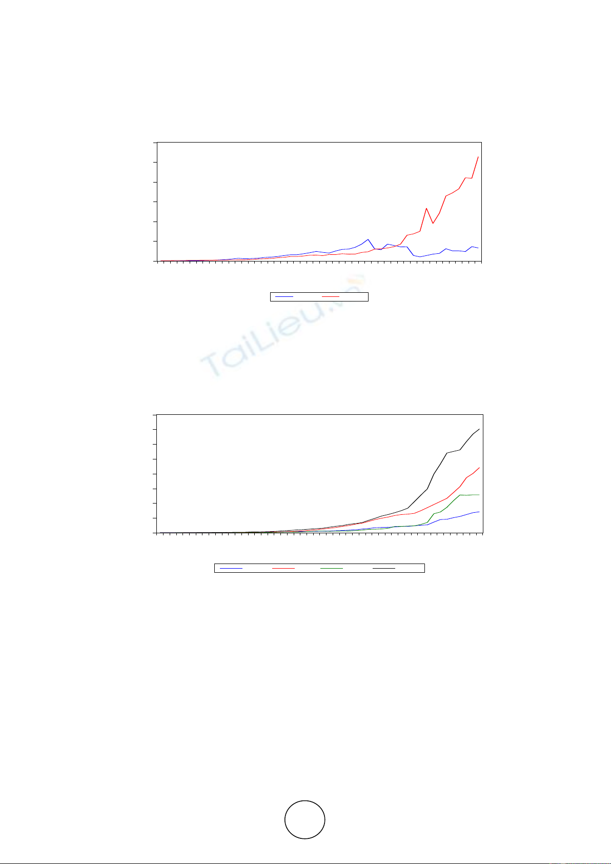
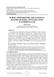
This study tried to empirically test the causal relationship and the direction of
causality between public expenditure and GDP in India, using annual data from 1966-
67 to 2015-16. The methodology employed was econometric model of the
cointegration and the Granger Causality test. The estimates shows that the variables
are stationary at first difference and follows I(1) order of integrations. Causality test
estimates shows bidirectional causal relationship running from GDP to Revenue
Expenditure and from Capital Expenditure to GDP. The estimates do not support the
existence of Keynesian hypothesis and Wagner’s Law at the disaggregate level in
India.
Key words: Public Expenditure, Wagner’s law, Keynesian hypothesis, Cointegration,
Granger Causality.
Cite this Article: Dhyani Mehta, Public Expenditure and National Income of India:
Investigating Wagnerian Law. International Journal of Management, 9 (5), 2018, pp.
19. http://www.iaeme.com/IJM/issues.asp?JType=IJM&VType=9&IType=5
1. INTRODUCTION
Can increase in public expenditure influence economic growth? What evidence exists on the
direct relationship between public expenditure and economic growth? There is lot of debate in
public finance literatures based on views of different school of thoughts in economics. There
are both theoretical and empirical evidence on the relationship between public expenditure
and Gross domestic product (GDP) growth (Blanchard, 2008). If public expenditure
negatively influences economic growth then policymakers need to be aware of these
relationships when formulating and implementing macroeconomic policy; and if public
expenditure enhances economic growth, or at a minimum does not present obstacles to
growth. However, it is important for policy makers to manage the debt, which arises due to
increased public expenditure and its impact on economy.
Public Expenditure is one of the important growth driver of any economy; GDP growth
should be sustained for a developing economy to address issues like unemployment, poverty,
inflation etc. Public expenditure plays a very crucial role in economic growth and stability.
Public Expenditure and National Income of India: Investigating Wagnerian Law
http://www.iaeme.com/IJM/index.asp 2 editor@iaeme.com
Public expenditure has been increasing over time in almost all the countries of the world; it is
very important for government to study the relation between GDP and public expenditure.
Increase or decrease in public expenditure will yield increase or decrease in economic growth
by increasing the national income, especially when it is injected in development programs
(Omoke, 2009).
If fiscal policy is applied through effective fiscal instruments like taxation and public
expenditure, it influences the working of the economic system and maximize economic
welfare with the overriding objective of promoting long-term growth of the economy (Tanzi,
1994). Fiscal policy and public finance has received much attention in the literature. There is
lot of debate on theoretical and empirical analysis on economic effects of public expenditures.
Some support a large public expenditure because it helps to put money into circulation,
increased investment and employment and reduces tax averseness etc. Others argues that
increase in public expenditure will lead to the fiscal deficit and creation of debt.
Government size has impact on economic growth; it has emerged as a major fiscal
management issue which is faced by economies in transition (Suleiman, 2009). The previous
research focuses on size of government in industrialized countries, but given the openness of
most developing countries, trade dependency, the vulnerability to external shocks, and
volatility of finances, the role and size of government become germane to adjustment and
stabilization programmes (Suleiman, 2009). There are two approaches on public expenditure
and economic growth relationship: Wagnerian’s law approach and Keynesians approach.
1.1. Wagnerian’s Law Approach
Wagner (1883) has introduced a model, which shows that public expenditures are endogenous
to economic growth, and that there exists long-run tendencies for public expenditure to grow
relatively to some national income aggregates such as GDP. This observation of Wagner led
to the Wagner’s law of increasing state activities. According to this law increased government
activity and public expenditure will lead to economic growth. Thus, it is said that causality
between public expenditure and national income runs from national income to public
expenditure.
1.2. Keynesians Approach
According to Keynes (1936) the government intervention by fiscal policies will help to
increase economic activities; thus public expenditure is an exogenous factor. The causal
relationship between public expenditure and national income runs from expenditure to
income. The main objective and focus of this paper is to study the components of public
expenditure which cause economic growth or vice versa. The long run tendencies that may
exist between of public expenditure and economic growth will be investigated using
cointegration and causality tests.
2. INDIA’S PUBLIC EXPENDITURE
Indian public expenditure can be classified into Revenue expenditure, which is recurrent in
nature. Revenue expenditure includes defence expenditure, interest payment, subsidies and
other-revenue expenditure. Capital expenditure is incurred on building durable assets in
economy. Capital expenditure is non-recurring in nature and includes loan and advances, and
capital outlay. Some of the examples of capital expenditure are expenditure on building river
dam projects, highways, steel plants, ports, buying of machinery and equipment, etc.
Figure-1 shows the revenue expenditures from year from 1966-67 to 2015-16; India’s
revenue expenditure has continuously grown over the period. Among the revenue
expenditure, other revenue expenditure (ORE) has highest growth rate followed by higher
Dhyani Mehta
http://www.iaeme.com/IJM/index.asp 3 editor@iaeme.com
growth rate of interest payment expenditure, due to increasing public and external debt.
Expenditure on subsidies also show increasing trend with objective of bringing equality and
efficiency in economic classes. India faces problem of terrorism and national security, which
lead to increase in defence expenditure.
Figure 1 Trend is Revenue Expenditure in India:
Source: Hand Book of Statistics Reserve Bank of India, 2015-16
Figure-2 show the real capital expenditures from year from 1966-67 to 2015-16. It is
clearly observed that India’s capital expenditure has been continuously growing over the
period of time. Among the capital expenditure loan and advances were having higher
proportion compared to capital out lay expenditure but it has shown downward trend.
Figure 2 Trend is Capital Expenditure in India
Source: Hand Book of Statistics Reserve Bank of India, 2015-16
Figure-3 shows comparison of percentage change GDP, with real figures of revenue
expenditure, capital expenditure, developmental expenditure and non-development
expenditure. There is highest fluctuation in percentage change in capital expenditure
compared to other public expenditure. Percentage change in GDP is showing a constant trend
with upward moment from year 2003-04.
0
400
800
1,200
1,600
2,000
2,400
1966-67
1968-69
1970-71
1972-73
1974-75
1976-77
1978-79
1980-81
1982-83
1984-85
1986-87
1988-89
1990-91
1992-93
1994-95
1996-97
1998-99
2000-01
2002-03
2004-05
2006-07
2008-09
2010-11
2012-13
2014-15
CLE COE
0
1,000
2,000
3,000
4,000
5,000
6,000
7,000
8,000
1966-67
1968-69
1970-71
1972-73
1974-75
1976-77
1978-79
1980-81
1982-83
1984-85
1986-87
1988-89
1990-91
1992-93
1994-95
1996-97
1998-99
2000-01
2002-03
2004-05
2006-07
2008-09
2010-11
2012-13
2014-15
RED IPE RSE ROE
Public Expenditure and National Income of India: Investigating Wagnerian Law
http://www.iaeme.com/IJM/index.asp 4 editor@iaeme.com
-60
-40
-20
0
20
40
60
80
1984-85
1985-86
1986-87
1987-88
1988-89
1989-90
1990-91
1991-92
1992-93
1993-94
1994-95
1995-96
1996-97
1997-98
1998-99
1999-00
2000-01
2001-02
2002-03
2003-04
2004-05
2005-06
2006-07
2007-08
2008-09
2009-10
2010-11
2011-12
2012-13
% Change GDP % Change CAP-EX
% Change DEV-EXP % Change REV-EX
% Change NDEV-EXP
Figure 3 Percentage Change in National Income & Public expenditure
Source: Hand Book of Statistics Reserve Bank of India, 2015-16
Graphical representation in Figure-1, Figure-2 and Figure-3 shows a positive relationship
between the GDP growth rate and the change in public expenditure in India i.e. an increase in
public expenditure and increase in growth rate within the considered period. This creates the
need for testing the direction of causality suggested by Wagnerian’s law and Keynesian
approach.
3. LITERATURE REVIEW
Extensive literature on theoretical and empirical debate between Wagner’s law and Keynesian
law tries to validate the causal relation between public expenditure and GDP. Singh and
Sahni (1984) examined causal link between public expenditure and national income on Indian
data and found bi-directional causality between public expenditure and national income.
Ahsan et al.(1992) studied United States data and failed to detect any causality between
public expenditure and national income. Afxentiou and Serletis (1996); Ansari et al. (1997)
and Abizadeh and Yousefi (1998) examined cross-country data, they were not able to find any
evidence supporting Wagner’s law. Bohl (1996) studied G7 countries (Post World War-II)
and found evidence for Wagner’s law for only countries like United Kingdom and Canada out
of G7 countries. Frimpong and Oteng-Abayie (2009) examined West African Monetary Zone
country data and results neither supported Wagner’s nor Keynesian view. Verma and Arora
(2010); and Ray (2012) examined causal relation between public expenditure and GDP on
Indian data and found short run causality between economic growth and public expenditure
supporting Wagner’s law.
Muhlis and Hakan (2003) used the natural log of annual data of Turkish economy from
1965-2000; co-integration and granger causality tests support neither Wagner’s Law nor
Keynes’ hypothesis. Jamshaid et al. (2010) examined direction of causality between public
expenditure with some selected expenditure components and national income of Pakistan;
Toda-Yamamoto causality test was used for annual data of 1971-2006, results concluded in
favour of Wagner’s law that there exists a unidirectional causality relationship flowing from
GDP to public expenditure. Olugbenga and Owoye (2007) used data from 1970-2005 of 30
OECD countries and found unidirectional and long-run relationship from public expenditure
to economic growth supporting Keynesian law for 16 countries. These were unidirectional
and long-run relationship between economic growth and public expenditure supporting
Wagner’s law observed for 10 countries, and four countries showed bi-causal relationship
between public expenditure and economic growth. Ergun and Tuck (2006) used Granger
causality test to investigate the causal links between the two variables for countries like
Dhyani Mehta
http://www.iaeme.com/IJM/index.asp 5 editor@iaeme.com
Indonesia, Malaysia, Philippines, Singapore, and Thailand, by using annual data from 1960-
2002 and found that causality runs from public expenditures to national income only for
Philippines.
The relationship between public expenditure and economic growth yields mix results and
the debate is never ending. It is very important for making policy to address issues like
recession, inflation, stagflation, unemployment, income inequality etc. It gives central
authorities ability to stimulate their economy through fiscal measures unless the share of
government spending to GNP increases or reduces. Knowing this long-run relationship helps
to make estimates of the public expenditure and national output and identify a benchmark
against which one can design the fiscal policy. The relationship between government
spending and national output is also important for the sustainability of public finances,
especially during the time when government is struggling to restrain spending. Thus the
identification of this relationship helps to provides a theoretical framework against which to
formulate and judge fiscal policy adjustment plans concerning medium term budgetary
objectives.
4. METHODOLOGY & DATA
Objective of this study is to test and bring out the evidence of the causal relationship between
public expenditure and GDP growth. Determinants of GPD growth is not taken in the study as
this paper only investigates primary long run relationship between GDP growth and
components of public expenditure. Granger (1969) proposed the concepts of causality using a
VAR model. In this study, Granger causality is used to investigate the causality between
public expenditures and GDP growth based on the VAR model. The data is taken from the
RBI’s Handbook of Statistics, 2015-16. The study uses natural log of annual data of GDP,
Revenue Expenditure and Capital Expenditure at disaggregate level for 50 years from year
1966 to 2016. Nominal variables are deflated into real ones by the GDP deflator (2004-05
constant price). Study uses test like ADF, Johansen cointegration test, Granger causality test.
Study includes seven variables i.e. GDP growth (Y), Variables for Revenue Expenditures are:
Defence Expenditure (RED), Interest payment (IPE), Subsidies (RSE), Others-revenue
Expenditure (ORE); Variables for Capital Expenditure are: Loan and Advances (CLE),
Capital Outlay = (COE). The Unit root test for stationarity, Johansen cointegration test and
Granger (1969) causality methodology were employed to determine the direction of causality
between public expenditure and GDP growth.
5. DATA ANALYSIS
5.1. Unit Root Tests
Any VAR model’s efficacy in establishing the relationship among variables is conditional on
the assumption of stationarity of the variables, which means variable should be made
stationary before conducting a Granger causality test based on the VAR. In case of non-
stationary time series, it implies the variables may be co-integrated. This means that
stationarity and co-integration test musts precede the Granger Causality test. According to
Greene (2003), the Augmented Dickey Fuller (ADF) test can be employed to test for unit root.
The results in Table-1 of ADF test show the order of integration of the variables and
presence of unit root. The variables are stationary at first difference, meaning that GDP (Y) is
stationary at I(1) first difference, Defence Expenditure (RDE), Interest payment (IPE),
Subsidies (RSE), Others-revenue Expenditure (ORE), Loan and Advances (CLE) and Capital
Outlay (COE); all values are natural log value stationary at I(1) first difference.