
EURASIP Journal on Applied Signal Processing 2005:15, 2470–2485
c
2005 Hindawi Publishing Corporation
Cosmological Non-Gaussian Signature Detection:
Comparing Performance of Different Statistical Tests
J. Jin
Department of Statistics, Purdue University, 150 N. University Street, West Lafayette, IN 47907, USA
Email: jinj@stat.purdue.edu
J.-L. Starck
DAPNIA/SEDI-SAP, Service d’Astrophysique, CEA-Saclay, 91191 Gif-sur-Yvette Cedex, France
Email: jstarck@cea.fr
D. L. Donoho
Department of Statistics, Stanford University, Sequoia Hall, Stanford, CA 94305, USA
Email: donoho@stat.stanford.edu
N. Aghanim
IAS-CNRS, Universit´
e Paris Sud, Bˆ
atiment 121, 91405 Orsay Cedex, France
Email: aghanim@ias.fr
Division of Theoretical Astronomy, National Astronomical Observatory of Japan, Osawa 2-21-1,
Mitaka, Tokyo 181-8588, Japan
O. Forni
IAS-CNRS, Universit´
e Paris Sud, Bˆ
atiment 121, 91405 Orsay Cedex, France
Email: olivier.forni@ias.fr
Received 30 June 2004
Currently, it appears that the best method for non-Gaussianity detection in the cosmic microwave background (CMB) consists
in calculating the kurtosis of the wavelet coefficients. We know that wavelet-kurtosis outperforms other methods such as the bis-
pectrum, the genus, ridgelet-kurtosis, and curvelet-kurtosis on an empirical basis, but relatively few studies have compared other
transform-based statistics, such as extreme values, or more recent tools such as higher criticism (HC), or proposed “best possible”
choices for such statistics. In this paper, we consider two models for transform-domain coefficients: (a) a power-law model, which
seems suited to the wavelet coefficients of simulated cosmic strings, and (b) a sparse mixture model, which seems suitable for the
curvelet coefficients of filamentary structure. For model (a), if power-law behavior holds with finite 8th moment, excess kurtosis
is an asymptotically optimal detector, but if the 8th moment is not finite, a test based on extreme values is asymptotically optimal.
For model (b), if the transform coefficients are very sparse, a recent test, higher criticism, is an optimal detector, but if they are
dense, kurtosis is an optimal detector. Empirical wavelet coefficients of simulated cosmic strings have power-law character, infinite
8th moment, while curvelet coefficients of the simulated cosmic strings are not very sparse. In all cases, excess kurtosis seems to
be an effective test in moderate-resolution imagery.
Keywords and phrases: cosmology, cosmological microwave background, non-Gaussianity detection, multiscale method, wavelet,
curvelet.
1. INTRODUCTION
The cosmic microwave background (CMB), discovered in
1965 by Penzias and Wilson [1], is a relic of radiation emit-
ted some 13 billion years ago, when the universe was about
370 000 years old. This radiation exhibits characteristic of an
almost perfect blackbody at a temperature of 2.726 kelvins
as measured by the FIRAS experiment on board COBE satel-
lite [2]. The DMR experiment, again on board COBE, de-
tected and measured angular small fluctuations of this tem-
perature, at the level of a few tens of microkelvins, and at
angular scale of about 10 degrees [3]. These so-called tem-
perature anisotropies were predicted as the imprints of the
initial density perturbations which gave rise to present large

Comparing Different Statistics in Non-Gaussian 2471
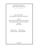
Figure 1: Courtesy of the WMAP team (reference to the website).
All sky map of the CMB anisotropies measured by the WMAP satel-
lite.
scale structures as galaxies and clusters of galaxies. This rela-
tion between the present-day universe and its initial condi-
tions has made the CMB radiation one of the preferred tools
of cosmologists to understand the history of the universe,
the formation and evolution of the cosmic structures, and
physical processes responsible for them and for their cluster-
ing.
As a consequence, the last several years have been a par-
ticularly exciting period for observational cosmology focus-
ing on the CMB. With CMB balloon-borne and ground-
based experiments such as TOCO [4], BOOMERanG [5],
MAXIMA [6], DASI [7], and Archeops [8],afirmdetection
of the so-called “first peak” in the CMB anisotropy angular
power spectrum at the degree scale was obtained. This detec-
tion has been very recently confirmed by the WMAP satel-
lite [9,10] (see Figure 1), which detected also the second and
third peaks. WMAP satellite mapped the CMB temperature
fluctuations with a resolution better than 15 arcminutes and
a very good accuracy marking the starting point of a new
era of precision cosmology that enables us to use the CMB
anisotropy measurements to constrain the cosmological pa-
rameters and the underlying theoretical models.
In the framework of adiabatic cold dark matter models,
the position, amplitude, and width of the first peak indeed
provide strong evidence for the inflationary predictions of a
flat universe and a scale-invariant primordial spectrum for
the density perturbations. Furthermore, the presence of sec-
ond and third peaks confirms the theoretical prediction of
acoustic oscillations in the primeval plasma and sheds new
light on various cosmological and inflationary parameters,
in particular, the baryonic content of the universe. The accu-
rate measurements of both the temperature anisotropies and
polarised emission of the CMB will enable us in the very near
future to break some of the degeneracies that are still affect-
ing parameter estimation. It will also allow us to probe more
directly the inflationary paradigm favored by the present ob-
servations.
Testing the inflationary paradigm can also be achieved
through detailed study of the statistical nature of the CMB
anisotropy distribution. In the simplest inflation models,
the distribution of CMB temperature fluctuations should be
Gaussian, and this Gaussian field is completely determined
by its power spectrum. However, many models such as mul-
tifield inflation (e.g., [11] and the references therein), su-
per strings, or topological defects predict non-Gaussian con-
tributions to the initial fluctuations [12,13,14]. The sta-
tistical properties of the CMB should discriminate mod-
els of the early universe. Nevertheless, secondary effects like
the inverse Compton scattering, the Doppler effect, lensing,
and others add their own contributions to the total non-
Gaussianity.
All these sources of non-Gaussian signatures might have
different origins and thus different statistical and morpho-
logical characteristics. It is therefore not surprising that a
large number of studies have recently been devoted to the
subject of the detection of non-Gaussian signatures. Many
approaches have been investigated: Minkowski functionals
and the morphological statistics [15,16], the bispectrum
(3-point estimator in the Fourier domain) [17,18,19],
the trispectrum (4-point estimator in the Fourier domain)
[20], wavelet transforms [21,22,23,24,25,26,27], and
the curvelet transform [27]. Different wavelet methods have
been studied, such as the isotropic `
a trous algorithm [28]
and the biorthogonal wavelet transform [29]. (The biorthog-
onal wavelet transform was found to be the most sensitive
to non-Gaussianity [27].) In [27,30], it was shown that the
wavelet transform was a very powerful tool to detect the non-
Gaussian signatures. Indeed, the excess kurtosis (4th mo-
ment) of the wavelet coefficients outperformed all the other
methods (when the signal is characterised by a nonzero 4th
moment).
Nevertheless, a major issue of the non-Gaussian studies
in CMB remains our ability to disentangle all the sources of
non-Gaussianity from one another. Recent progress has been
made on the discrimination between different possible ori-
gins of non-Gaussianity. Namely, it was possible to separate
the non-Gaussian signatures associated with topological de-
fects (cosmic strings (CS)) from those due to Doppler effect
of moving clusters of galaxies (both dominated by a Gaussian
CMB field) by combining the excess kurtosis derived from
both the wavelet and the curvelet transforms [27].
This success argues for us to construct a “toolkit” of well-
understood and sensitive methods for probing different as-
pects of the non-Gaussian signatures.
In that spirit, the goal of the present study is to consider
the advantages and limitations of detectors which apply kur-
tosis to transform coefficients of image data. We will study
plausible models for transform coefficients of image data and
compare the performance of tests based on kurtosis of trans-
form coefficients to other types of statistical diagnostics.
At the center of our analysis are the following two facts:
(A) the wavelet/curvelet coefficients of CMB are Gaussian
(we implicitly assume the most simple inflationary
scenario);
(B) the wavelet/curvelet coefficients of topological defect
and Doppler effect simulations are non-Gaussian.
We develop tests for non-Gaussianity for two models of
statistical behavior of transform coefficients. The first, better
suited for wavelet analysis, models transform coefficients of
cosmic strings as following a power law. The second, theoret-
ically better suited for curvelet coefficients, assumes that the

2472 EURASIP Journal on Applied Signal Processing
salient features of interest are actually filamentary (it can be
residual strips due to a nonperfect calibration), which gives
the curvelet coefficients a sparse structure.
We review some basic ideas from detection theory, such
as likelihood ratio detectors, and explain why we prefer non-
parametric detectors, valid across a broad range of assump-
tions.
In the power-law setting, we consider two kinds of non-
parametric detectors. The first, based on kurtosis, is asymp-
totically optimal in the class of weakly dependent symmetric
non-Gaussian contamination with finite 8th moments. The
second, the Max, is shown to be asymptotically optimal in the
class of weakly dependent symmetric non-Gaussian contam-
ination with infinite 8th moment. While the evidence seems
to be that wavelet coefficients of CS have about 6 existing
moments, indicating a decisive advantage for extreme-value
statistics, the performance of kurtosis-based tests and Max-
based tests on moderate sample sizes (e.g., 64 K transform
coefficients) does not follow the asymptotic theory; excess
kurtosis works better at these sample sizes.
In the sparse-coefficients setting, we consider kurtosis,
the Max, and a recent statistic called higher criticism (HC)
[31]. Theoretical analysis suggests that curvelet coefficients
of filamentary features should be sparse, with about n1/4sub-
stantial nonzero coefficients out of ncoefficients in a sub-
band; this level of sparsity would argue in favor of Max/HC.
However, empirically, the curvelet coefficients of actual CS
simulations are not very sparse. It turns out that kurtosis out-
performs Max/HC in simulation.
Summarizing, the work reported here seems to show
that for all transforms considered, the excess kurtosis out-
performs alternative methods despite their strong theoreti-
cal motivation. A reanalysis of the theory supporting those
methods shows that the case for kurtosis can also be justi-
fied theoretically based on observed statistical properties of
the transform coefficients not used in the original theoretic
analysis.
2. DETECTING FAINT NON-GAUSSIAN SIGNALS
SUPERPOSED ON A GAUSSIAN SIGNAL
The superposition of a non-Gaussian signal with a Gaussian
signal can be modeled as Y=N+G,whereYis the ob-
served image, Nis the non-Gaussian component, and Gis
the Gaussian component. We are interested in using trans-
form coefficients to test whether N≡0ornot.
2.1. Hypothesis testing and likelihood ratio test
Transfor m coefficients of various kinds (Fourier, wavelet,
etc.) have been used for detecting non-Gaussian behavior in
numerous studies. Let X1,X2,...,Xnbe the transform coeffi-
cients of Y; we model these as
Xi=1−λ·zi+λ·wi,0<λ<1, (1)
where λ>0isaparameter,ziiid
∼N(0, 1) are the trans-
form coefficients of the Gaussian component G,wiiid
∼Ware
the transform coefficients of the non-Gaussian component
N,andWis some unknown symmetrical distribution. Here
without loss of generality, we assume the standard deviation
for both ziand wiis 1.
Phrased in statistical terms, the problem of detecting the
existence of a non-Gaussian component is equivalent to dis-
criminating between the hypotheses
H0:Xi=zi,(2)
H1:Xi=1−λ·zi+λ·wi,0<λ<1, (3)
and N≡0isequivalenttoλ≡0. We call H0the null hypoth-
esis and H1the alternative hypothesis.
When both Wand λare known, then the optimal test for
problem (2)-(3) is simply the Neyman-Pearson likelihood
ratio test (LRT) [32,page74].Thesizeofλ=λnfor which
reliable discrimination between H0and H1is possible can be
derived using asymptotics. If we assume that the tail proba-
bility of Wdecays algebraically,
lim
x→∞ xαP{|W|>x}=Cα,Cαis a constant (4)
(we say Whas a power-law tail), and we calibrate λto de-
cay with n, so that increasing amounts of data are offset by
increasingly hard challenges:
λ=λn=n−r,(5)
then there is a threshold effect for the detection problem (2)-
(3). In fact, define
ρ∗
1(α)=
2
α,α≤8,
1
4,α>8,
(6)
then, as n→∞, LRT is able to reliably detect for large nwhen
r<ρ
∗
1(α), and is unable to detect when r>ρ
∗
1(α); this is
proved in [33]. Since LRT is optimal, it is not possible for
any statistic to reliably detect when r>ρ
∗
1(α). We call the
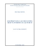
curve r=ρ∗
1(α) in the α-rplane the detection boundary;see
Figure 2.
In fact, when r<1/4, asymptotically LRT is able to reli-
ably detect whenever Whas a finite 8th moment, even with-
out the assumption that Whas a power-law tail. Of course,
the case that Whas an infinite 8th moment is more compli-
cated, but if Whas a power-law tail, then LRT is also able to
reliably detect if r<2/α.
Despite its optimality, LRT is not a practical procedure.
To apply LRT, one needs to specify the value of λand the
distribution of W, which seems unlikely to be available. We
need nonparametric detectors, which can be implemented
without any knowledge of λor W, and depend on Xi’s
only. In the section below, we are going to introduce two
nonparametric detectors: excess kurtosis and Max; later in
Section 4.3, we will introduce a third nonparametric detec-
tor: higher criticism (HC).

Comparing Different Statistics in Non-Gaussian 2473
1
0.9
0.8
0.7
0.6
0.5
0.4
0.3
0.2
0.1
0
r
2 4 6 8 10 12 14 16 18
α
Undetectable
Detectable
for Max/HC
not for kurtosis
Detectable for kurtosis
not for Max/HC
Detectable for both kurtosis and Max/HC
Figure 2: Detectable regions in the α-rplane. With (α,r)inthe
white region on the top or in the undetectable region, all methods
completely fail for detection. With (α,r) in the white region on the
bottom, both excess kurtosis and Max/HC are able to detect reliably.
In the shaded region to the left, Max/HC is able to detect reliably,
but excess kurtosis completely fails, and in the shaded region to the
right, excess kurtosis is able to detect reliably, but Max/HC com-
pletely fails.
2.2. Excess kurtosis and Max
We pause to review the concept of p-value briefly. For a
statistic Tn, the p-value is the probability of seeing equally
extreme results under the null hypothesis:
p=PH0Tn≥tnX1,X2,...,Xn;(7)
here PH0refers to probability under H0,and
tn(X1,X2,...,Xn) is the observed value of statistic Tn.
Notice that the smaller the p-value, the stronger the evidence
against the null hypothesis. A natural decision rule based
on p-values rejects the null when p<αfor some selected
level α, and a convenient choice is α=5%. When the null
hypothesis is indeed true, the p-values for any statistic
are distributed as uniform U(0, 1). This implies that the
p-values provide a common scale for comparing different
statistics.
We now introduce two statistics for comparison.
Excess kurtosis (κn)
Excess kurtosis is a widely used statistic, based on the 4th mo-
ment. For any (symmetrical) random variable X, the kurtosis
is
κ(X)=EX4
EX22−3.(8)
The kurtosis measures a kind of departure of Xfrom Gaus-
sianity, as κ(z)=0.
Empirically, given nrealizations of X, the excess kurtosis
statistic is defined as
κnX1,X2,...,Xn=n
24 (1/n)iX4
i
(1/n)iX2
i2−3.(9)
When the null is true, the excess kurtosis statistic is asymp-
totically normal:
κnX1,X2,...,Xn−→ wN(0, 1), n−→ ∞ , (10)
thus for large n, the p-value of the excess kurtosis is approxi-
mately
˜
p=¯
Φ−1κnX1,X2,...,Xn, (11)
where ¯
Φ(·) is the survival function (upper-tail probability)
of N(0, 1).
It is proved in [33] that the excess kurtosis is asymptoti-
cally optimal for the hypothesis testing of (2)-(3)if
EW8<∞.(12)
However, when E[W8]=∞, even though kurtosis is well
defined (E[W4]<∞), there are situations in which LRT is
able to reliably detect but excess kurtosis completely fails. In
fact, by assuming (4)-(5)withanα<8, if (α,r) falls into
the shaded region to the left of Figure 2, then LRT is able to
reliably detect, however, excess kurtosis completely fails. This
shows that in such cases, excess kurtosis is not optimal; see
[33].
Max (Mn)
The largest (absolute) observation is a classical and fre-
quently used nonparametric statistic:
Mn=max
X1
,
X2
,...,
Xn
, (13)
under the null hypothesis,
Mn≈2logn, (14)
and, moreover, by normalizing Mnwith constants cnand dn,
the resulting statistic converges to the Gumbel distribution
Ev, whose cdf is e−e−x:
Mn−cn
dn−→ wEv, (15)
where approximately
dn=√6Sn
π,cn=¯
X−0.5772dn; (16)
here ¯
Xand Snare the sample mean and sample standard de-
viation of {Xi}n
i=1, respectively. Thus a good approximation
of the p-value for Mnis
˜
p=exp −exp −Mn−cn
dn.(17)
We have tried the above experiment for n=2442,andfound
that taking cn=4.2627, dn=0.2125 gives a good approxi-
mation.

2474 EURASIP Journal on Applied Signal Processing
Assuming (4)-(5)andα<8, or λ=n−r, and that Whas
a power-law tail with α<8, it is proved in [33] that Max
is optimal for hypothesis testing (2)-(3). Recall if we further
assume 1/4<r<2/α, then asymptotically excess kurtosis
completely fails; however, Max is able to reliably detect and is
competitive to LRT.
On the other hand, recall that excess kurtosis is optimal
for the case α>8. In comparison, in this case, Max is not op-
timal. In fact, if we further assume 2/α < r < 1/4, then excess
kurtosis is able to reliably detect, but Max will completely fail.
In Figure 2, we compared the detectable regions of the
excess kurtosis and Max in the α-rplane.
To conclude this section, we mention an alternative way
to approximate the p-values for any statistic Tn. This alterna-
tive way is important in case that an asymptotic (theoretic)
approximation is poor for moderate large n, an example is
the statistic HC∗
nwe will introduce in Section 4.3; this alter-
native way is helpful even when the asymptotic approxima-
tion is accurate. Now the idea is that, under the null hypoth-
esis, we simulate a large number (N=104or more) of Tn:
T(1)
n,T(2)
n,...,T(N)
n, we then tabulate them. For the observed
value tn(X1,X2,...,Xn), the p-value will then be well approx-
imated by
1
N·#k:T(k)
n≥tnX1,X2,...,Xn, (18)
and the larger the N, the better the approximation.
2.3. Heuristic approach
We have exhibited a phase-change phenomenon, where the
asymptotically optimal test changes depending on power-law
index α. In this section, we develop a heuristic analysis of
detectability and phase change.
The detection property of Max follows from compar-
ing the ranges of data. Recall that Xi=1−λn·zi+
λn·wi, the range of {zi}n
i=1is roughly (−2logn,2logn),
and the range of {λn·wi}n
i=1is λn·(−n1/α,n1/α)=
(−n1/α−r/2,n1/α−r/2); so, heuristically,
Mn≈max 2logn,n1/α−r/2; (19)
for large n, notice that
n1/α−r/2≫2logn,ifr<2
α,
n1/α−r/2≪2logn,ifr>2
α,
(20)
thus if and only if r<2/α,Mnfor the alternative will differ
significantly from Mnfor the null, and so the criterion for
detectability by Max is r<2/α.
Now we study detection by excess kurtosis. Heuristically,
κn≈1
√24 ·κ1−λn·zi+λn·wi
=1
√24 ·√n·λ2
n·κ(W)=On1/2−2r,
(21)
thus if and only if r<1/4, κnfor the alternative will differ
significantly from κnunder the null, and so the criterion for
detectability by excess kurtosis is r<1/4.
This analysis shows the reason for the phase change. In
Figure 2, when the parameter (α,r) is in the shaded region to
the left, for sufficiently large n,n1/α−r/2≫2lognand the
strongest evidence against the null is in the tails of the data
set, which Mnis indeed using. However, when (α,r)moves
from the shaded region to the left to the shaded region to
the right, n1/α−r/2≪2logn, the tails no longer contain any
important evidence against the null, instead, the central part
of the data set contains the evidence. By symmetry, the 1st
and the 3rd moments vanish, and the 2nd moment is 1 by
the normalization; so the excess kurtosis is in fact the most
promising candidate of detectors based on moments.
The heuristic analysis is the essence for theoretic proof
as well as empirical experiment. Later in Section 3.4,wewill
have more discussions for comparing the excess kurtosis with
Max down this vein.
3. WAVELET COEFFICIENTS OF COSMIC STRINGS
3.1. Simulated astrophysical signals
The temperature anisotropies of the CMB contain the con-
tributions of both the primary cosmological signal, directly
related to the initial density perturbations, and the secondary
anisotropies. The latter are generated after matter-radiation
decoupling [34]. They arise from the interaction of the CMB
photons with the neutral or ionised matter along their path
[35,36,37].
In the present study, we assume that the primary CMB
anisotropies are dominated by the fluctuations generated
in the simple single field inflationary cold-dark-matter
model with a nonzero cosmological constant. The CMB
anisotropies have therefore a Gaussian distribution. We al-
low for a contribution to the primary signal from topological
defects, namely, cosmic strings (CS), as suggested in [38,39].
See Figures 3and 4.
We use for our simulations the cosmological parame-
ters obtained from the WMAP satellite [10]andanormal-
ization parameter σ8=0.9. Finally, we obtain the so-called
“simulated observed map,” D, that contains the two pre-
vious astrophysical components. It is obtained from Dλ=
√1−λCMB + √λCS, where CMB and CS are, respectively,
the CMB and the cosmic string simulated maps. λ=0.18
is an upper limit constant derived by [38]. All the simulated
maps have 500 ×500 pixels with a resolution of 1.5 arcmin-
utes per pixel.
3.2. Evidence for E[W8]=∞
For the wavelet coefficients on the finest scale of the cosmic
string map in Figure 3b, by throwing away all the coefficients
related to pixels on the edge of the map, we have n=2442
coefficients; we then normalize these coefficients so that the
empirical mean and standard deviation are 0 and 1, respec-
tively; we denote the resulting dataset by {wi}n
i=1.


%20--%3e%3cdefs%3e%3cstyle%3e%20.st0%20{%20fill:%20%23fff;%20}%20.st1%20{%20fill:%20%237800fa;%20}%20%3c/style%3e%3c/defs%3e%3cpath%20class='st1'%20d='M117.78,12.18H43.11c2.9,3.47,4.65,7.94,4.65,12.82,0,5.6-2.3,10.66-6.01,14.29h76.02l7.22-13.56-7.22-13.56Z'/%3e%3cg%3e%3cpath%20class='st0'%20d='M53.58,26.17h-.59v-1.46h.59v-4.96h2.83c1.78,0,2.67.94,2.67,2.82v5.76c0,1.87-.89,2.81-2.67,2.81h-2.83v-4.96ZM55.36,21.37v3.34h1.1v1.46h-1.1v3.34h1.01c.61,0,.91-.37.91-1.1v-5.93c0-.74-.3-1.1-.91-1.1h-1.01Z'/%3e%3cpath%20class='st0'%20d='M65.99,31.14h-1.8l-.31-2.07h-2.19l-.31,2.07h-1.64l1.82-11.39h2.62l1.82,11.39ZM65.28,18.04c-.25.46-.51.77-.75.94-.21.15-.47.22-.79.22-.26,0-.57-.07-.92-.22l-.38-.15c-.14-.05-.26-.07-.37-.07-.3,0-.53.18-.71.54l-.91-.68c.25-.46.51-.77.75-.94.21-.14.48-.21.79-.21.26,0,.57.07.92.21l.38.15c.14.05.26.07.37.07.3,0,.53-.18.71-.54l.91.68ZM61.91,27.52h1.73l-.87-5.76-.87,5.76Z'/%3e%3cpath%20class='st0'%20d='M74.53,26.89v1.52c0,1.91-.89,2.86-2.67,2.86s-2.67-.95-2.67-2.86v-5.93c0-1.91.89-2.86,2.67-2.86s2.67.95,2.67,2.86v1.11h-1.69v-1.22c0-.75-.31-1.12-.93-1.12s-.93.37-.93,1.12v6.15c0,.74.31,1.11.93,1.11s.93-.37.93-1.11v-1.63h1.69Z'/%3e%3cpath%20class='st0'%20d='M81.4,31.14h-1.8l-.31-2.07h-2.19l-.31,2.07h-1.64l1.82-11.39h2.62l1.82,11.39ZM75.9,19.2l1.52-1.91h1.71l1.51,1.91h-1.61l-.76-.95-.75.95h-1.61ZM77.32,27.52h1.73l-.87-5.76-.87,5.76ZM83.1,15.99l-1.76,1.91h-1.26l1.17-1.91h1.86Z'/%3e%3cpath%20class='st0'%20d='M84.86,19.75c1.78,0,2.67.94,2.67,2.82v1.48c0,1.87-.89,2.81-2.67,2.81h-.85v4.28h-1.79v-11.39h2.64ZM84.01,21.37v3.86h.85c.58,0,.87-.36.87-1.08v-1.71c0-.71-.29-1.07-.87-1.07h-.85Z'/%3e%3cpath%20class='st0'%20d='M93.51,19.75c1.78,0,2.67.94,2.67,2.82v1.48c0,1.87-.89,2.81-2.67,2.81h-.85v4.28h-1.79v-11.39h2.64ZM92.66,21.37v3.86h.85c.58,0,.87-.36.87-1.08v-1.71c0-.71-.29-1.07-.87-1.07h-.85Z'/%3e%3cpath%20class='st0'%20d='M98.8,31.14h-1.79v-11.39h1.79v4.88h2.03v-4.88h1.83v11.39h-1.83v-4.88h-2.03v4.88Z'/%3e%3cpath%20class='st0'%20d='M105.36,24.55h2.46v1.62h-2.46v3.34h3.09v1.63h-4.88v-11.39h4.88v1.63h-3.09v3.18ZM108.17,17.29l-1.76,1.91h-1.26l1.17-1.91h1.86Z'/%3e%3cpath%20class='st0'%20d='M112.2,19.75c1.78,0,2.67.94,2.67,2.82v1.48c0,1.87-.89,2.81-2.67,2.81h-.85v4.28h-1.79v-11.39h2.64ZM111.35,21.37v3.86h.85c.58,0,.87-.36.87-1.08v-1.71c0-.71-.29-1.07-.87-1.07h-.85Z'/%3e%3c/g%3e%3ccircle%20class='st1'%20cx='25'%20cy='25'%20r='20'/%3e%3cpath%20class='st0'%20d='M32.78,19.27c2.92,0,4.43,2.55,5.28,5.33l.71,2.17c.14.38-.33.75-.71.75h-5.61c.19-.33.24-.71.09-1.08l-.75-2.45c-.43-1.32-.99-2.64-1.79-3.77.75-.57,1.65-.94,2.78-.94h0ZM25,18.38c3.25,0,4.9,2.78,5.89,5.89l.76,2.45c.14.42-.33.8-.8.8h-11.69c-.42,0-.94-.38-.8-.8l.75-2.45c.99-3.11,2.64-5.89,5.89-5.89h0ZM25,11.35c1.74,0,3.11,1.37,3.11,3.11s-1.37,3.11-3.11,3.11-3.11-1.41-3.11-3.11,1.41-3.11,3.11-3.11h0ZM17.27,19.27c1.08,0,1.98.38,2.73.94-.8,1.13-1.37,2.45-1.74,3.77l-.8,2.45c-.14.38-.05.75.09,1.08h-5.56c-.42,0-.9-.38-.75-.75l.71-2.17c.9-2.78,2.41-5.33,5.33-5.33h0ZM17.27,12.91c1.51,0,2.78,1.27,2.78,2.83s-1.27,2.83-2.78,2.83-2.83-1.27-2.83-2.83,1.27-2.83,2.83-2.83h0ZM32.78,12.91c1.56,0,2.78,1.27,2.78,2.83s-1.23,2.83-2.78,2.83-2.83-1.27-2.83-2.83,1.27-2.83,2.83-2.83h0ZM27.07,28.56v.09c0,.57-.24,1.08-.61,1.46h0v.05c-.38.33-.9.57-1.46.57s-1.08-.24-1.46-.61h0c-.38-.38-.61-.9-.61-1.46v-.09h1.41v.09c0,.19.05.38.19.47v.05c.09.09.28.19.47.19s.38-.09.47-.19v-.05c.14-.09.24-.28.24-.47t-.05-.09h1.41ZM30.99,28.56v.09c0,1.65-.66,3.16-1.74,4.24-1.08,1.08-2.59,1.79-4.24,1.79s-3.16-.71-4.24-1.79l-.05-.05c-1.04-1.08-1.7-2.55-1.7-4.2v-.09h1.41v.09c0,1.27.47,2.4,1.27,3.25h.05c.85.85,1.98,1.37,3.25,1.37s2.4-.52,3.25-1.37c.85-.8,1.37-1.98,1.37-3.25v-.09h1.37ZM34.99,28.56v.09c0,2.78-1.13,5.28-2.92,7.07-1.79,1.79-4.29,2.92-7.07,2.92s-5.23-1.13-7.07-2.92c-1.79-1.79-2.92-4.29-2.92-7.07v-.09h1.41v.09c0,2.4.94,4.53,2.5,6.08,1.56,1.56,3.72,2.5,6.08,2.5s4.52-.94,6.08-2.5c1.56-1.56,2.5-3.68,2.5-6.08v-.09h1.41Z'/%3e%3c/svg%3e)