
Hindawi Publishing Corporation
EURASIP Journal on Advances in Signal Processing
Volume 2007, Article ID 89354, 11 pages
doi:10.1155/2007/89354
Research Article
A MAP Estimator for Simultaneous Superresolution and
Detector Nonunifomity Correction
Russell C. Hardie1and Douglas R. Droege2
1Department of Electrical and Computer Engineering, University of Dayton, 300 College Park, Dayton, OH 45469-0226, USA
2L-3 Communications Cincinnati Electronics, 7500 Innovation Way, Mason, OH 45040, USA
Received 31 August 2006; Accepted 9 April 2007
Recommended by Richard R. Schultz
During digital video acquisition, imagery may be degraded by a number of phenomena including undersampling, blur, and noise.
Many systems, particularly those containing infrared focal plane array (FPA) sensors, are also subject to detector nonuniformity.
Nonuniformity, or fixed pattern noise, results from nonuniform responsivity of the photodetectors that make up the FPA. Here we
propose a maximum a posteriori (MAP) estimation framework for simultaneously addressing undersampling, linear blur, additive
noise, and bias nonuniformity. In particular, we jointly estimate a superresolution (SR) image and detector bias nonuniformity
parameters from a sequence of observed frames. This algorithm can be applied to video in a variety of ways including using a mov-
ing temporal window of frames to process successive groups of frames. By combining SR and nonuniformity correction (NUC)
in this fashion, we demonstrate that superior results are possible compared with the more conventional approach of performing
scene-based NUC followed by independent SR. The proposed MAP algorithm can be applied with or without SR, depending on
the application and computational resources available. Even without SR, we believe that the proposed algorithm represents a novel
and promising scene-based NUC technique. We present a number of experimental results to demonstrate the efficacy of the pro-
posed algorithm. These include simulated imagery for quantitative analysis and real infrared video for qualitative analysis.
Copyright © 2007 R. C. Hardie and D. R. Droege. This is an open access article distributed under the Creative Commons
Attribution License, which permits unrestricted use, distribution, and reproduction in any medium, provided the original work is
properly cited.
1. INTRODUCTION
During digital video acquisition, imagery may be degraded
by a number of phenomena including undersampling, blur,
and noise. Many systems, particularly those containing
infrared focal plane array (FPA) sensors, are also subject to
detector nonuniformity [1–4]. Nonuniformity, or fixed pat-
tern noise, results from nonuniform responsivity of the pho-
todetectors that make up the FPA. This nonuniformity tends
to drift over time, precluding a simple one-time factory cor-
rection from completely eradicating the problem. Traditional
methods of reducing fixed pattern noise, such as correlated
double sampling [5], are often ineffective because the pro-
cessing technology and operating temperatures of infrared
sensor materials result in the dominance of different sources
of nonuniformity. Periodic calibration techniques can be em-
ployed to address the problem in the field. These, however,
require halting normal operation while the imager is aimed
at calibration targets. Furthermore, these methods may only
be effective for a scene with a dynamic range close to that
of the calibration targets. Many scene-based techniques have
been proposed to perform nonuniformity correction (NUC)
using only the available scene imagery (without calibration
targets).
Some of the first scene-based NUC techniques were based
on the assumption that the statistics of each detector output
should be the same over a sufficient number of frames as
long as there is motion in the scene. In [6–9], offset and
gain correction coefficients are estimated by assuming that
the temporal mean and variance of each detector are identi-
cal over time. Both a temporal highpass filtering approach
that forces the mean of each detector to zero and a least-
mean squares technique that forces the output of a pixel
to be similar to its neighbors are presented in [10–12]. By
exploiting a local constant statistics assumption, the tech-
nique presented in [13] treats the nonuniformity at the de-
tector level separately from the nonuniformity in the read-
out electronics. Another approach is based on the assump-
tion that the output of each detector should exhibit a con-
stant range of values [14]. A Kalman filter-based approach

2 EURASIP Journal on Advances in Signal Processing
that exploits the constant range assumption has been pro-
posed in [15]. A nonlinear filter-based method is described
in [16]. As a group, these methods are often referred to as
constant statistics techniques. Constant statistics techniques
work well when motion in a relatively large number of frames
distributes diverse scene intensities across the FPA.
Another set of proposed scene-based NUC techniques
utilizes motion estimation or specific knowledge of the
relative motion between the scene and the FPA [17–23].
A motion-compensated temporal average approach is pre-
sented in [19]. Algebraic scene-based NUC techniques are
developedin[20–22]. A regularized least-squares method,
closely related to this work, is presented in [23]. These
motion-compensated techniques are generally able to op-
erate successfully with fewer frames than constant statis-
tics techniques. Note that many motion-compensated tech-
niques utilize interpolation to treat subpixel motion. If the
observed imagery is undersampled, the ability to perform ac-
curate interpolation is compromised, and these NUC tech-
niques can be adversely affected.
When aliasing from undersampling is the primary form
of degradation, a variety of superresolution (SR) algorithms
can be employed to exploit motion in digital video frames. A
good survey of the field can be found in [24,25]. Statistical
SR estimation methods derived using a Bayesian framework,
similar to that used here, include [26–30]. When significant
levels of both nonuniformity and aliasing are present, most
approaches treat the nonuniformity and undersampling sep-
arately. In particular, some type of calibration or scene-based
NUC is employed initially. This is followed by applying an SR
algorithm to the corrected imager [31,32]. One pioneering
paper developed a maximum-likelihood estimator to jointly
estimate a high-resolution (HR) image, shift parameters, and
nonuniformity parameters [33].
Here we combine scene-based NUC with SR using a max-
imum a posteriori (MAP) estimation framework to jointly
estimate an SR image and detector nonuniformity param-
eters from a sequence of observed frames (MAP SR-NUC
algorithm). We use Gaussian priors for the HR image, bi-
ases, and noise. We employ a gradient descent optimization
and estimate the motion parameters prior to the MAP algo-
rithm. Here we focus on translational and rotational motion.
The joint MAP SR-NUC algorithm can be applied to video
in a variety of ways including processing successive groups
of frames spanned by a moving temporal window of frames.
By combining SR and NUC in this fashion, we demonstrate
that superior results are possible compared with the more
conventional approach of performing scene-based NUC fol-
lowed by independent SR. This is because access to an SR
image can make interpolation more accurate, leading to im-
proved nonuniformity parameter estimation. Similarly, HR
image estimation requires accurate knowledge of the detector
nonuniformity parameters. The proposed MAP algorithm
can be applied with or without SR, depending on the ap-
plication and computational resources available. Even with-
out SR, we believe that the proposed algorithm represents
a novel and promising scene-based NUC technique (MAP
NUC algorithm).
yk=Wkz+b+nk
zyk
Wkbnk
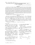
Motion PSF ↓Lx↓Ly
Figure 1: Observation model for simultaneous image superresolu-
tion and nonuniformity correction.
The rest of this paper is organized as follows. In Section 2,
we present the observation model. The joint MAP estimator
and corresponding optimization are presented in Section 3.
Experimental results are presented in Section 4 to demon-
strate the efficacy of the proposed algorithm. These include
results produced using simulated imagery for quantitative
analysis and real infrared video for qualitative analysis. Con-
clusions are presented in Section 5.
2. OBSERVATION MODEL
Figure 1 illustrates the observation model that relates a set
of observed low-resolution (LR) frames with a correspond-
ing desired HR image. Sampling the scene at or above the
Nyquist rate gives rise to the desired HR image, denoted us-
ing lexicographical notation as an N×1vectorz. Next, a
geometric transformation is applied to model the relative
motion between the camera and the scene. Here we con-
sider rigid translational and rotational motion. This requires
only three motion parameters per frame and is a reason-
ably good model for video of static scenes imaged at long
range from a nonstationary platform. We next incorporate
the point spread function (PSF) of the imaging system using
a 2D linear convolution operation. The PSF can be modi-
fied to include other degradations as well. In the model, the
image is then downsampled by factors of Lxand Lyin the
horizontal and vertical directions, respectively.
We now introduce the nonuniformity by adding an M×1
array of biases, b,whereM=N/(LxLy). Detector nonunifor-
mity is frequently modeled using a gain parameter and bias
parameter for each detector, allowing for a linear correction.
However, in many systems, the nonuniformity in the gain
term tends to be less variable and good results can be ob-
tained from a bias-only correction. Since a model containing
only biases simplifies the resulting algorithms and provides
good results on the imagery tested here, we focus here on a
bias-only nonuniformity model. Finally, an M×1 Gaussian
noise vector nkis added. This forms the kth observed frame
represented by an M×1vectoryk. Let us assume that we have
observed Pframes, y1,y2,...,yP. The complete observation
model can be expressed as
yk=Wkz+b+nk,(1)
for k=1, 2, ...,P,whereWkis an M×Nmatrix that imple-
ments the motion model for the kth frame, the system PSF

R. C. Hardie and D. R. Droege 3
blur, and the subsampling shown in Figure 1. Note that this
model can accommodate downsampling (i.e., Lx,Ly>1) for
SR or can perform NUC only for Lx=Ly=1. Also note that
the operation Wkzimplements subpixel motion for any Lx
and Lyby performing bilinear interpolation.
We model the additive noise as a zero-mean Gaussian
random vector with the following multivariate PDF:
Pr nk=1
(2π)M/2σM
n
exp −1
2σ2
n
nT
knk,(2)
for k=1, 2, ...,P,whereσ2
nis the noise variance. We also as-
sume that these random vectors are independent from frame
to frame (temporal noise).
We model the biases (fixed pattern noise) as a zero-mean
Gaussian random vector with the following PDF:
Pr b=1
(2πM/2σM
b
exp −1
2σ2
b
bTb,(3)
where σ2
bis the variance of the bias parameters. This Gaus-
sian model is chosen for analytical convenience but has been
shown to produce useful results.
We model the HR image using a Gaussian PDF given by
Pr(z=1
(2π)N/2
Cz
1/2exp −1
2zTC−1
zz,(4)
where Czis the N×Ncovariance matrix. The exponential
term in (4) can be factored into a sum of products yielding
Pr(z)=1
(2π)N/2
Cz
1/2exp −1
2σ2
z
N
i=1
zTdidT
iz,(5)
where di=[di,1,di,2,...,di,N]Tis a coefficient vector. Thus,
the prior can be rewritten as
Pr(z)=1
(2π)N/2
Cz
1/2exp −1
2σ2
z
N
i=1N
j=1
di,jzj2.
(6)
The coefficient vectors difor i=1, 2, ...,Nare selected to
provide a higher probability for smooth random fields. Here
we have selected the following values for the coefficient vec-
tors:
di,j=⎧
⎪
⎨
⎪
⎩
1fori=j,
−1
4for j:zjis a cardinal neighbor of zi.(7)
This model implies that every pixel value in the desired image
can be modeled as the average of its four cardinal neighbors
plus a Gaussian random variable of variance σ2
z. Note that
the prior in (6) can also be viewed as a Gibbs distribution
where the exponential term is a sum of clique potential func-
tions [34] derived from a third-order neighborhood system
[35,36].
3. JOINT SUPERRESOLUTION AND
NONUNIFORMITY CORRECTION
Given that we observe Pframes, denoted by y=
[yT
1,yT
2,...,yT
P]T, we wish to jointly estimate the HR image
zand the nonuniformity parameters b.InSection 4,wewill
demonstrate that it is advantageous to estimate these simul-
taneously versus independently.
3.1. MAP estimation
The joint MAP estimation is given by
z,
b=arg max
z,b
Pr(z,b|y).(8)
Using Bayes rule, this can be equivalently be expressed as
z,
b=arg max
z,b
Pr(y|z,b)Pr(z,b)
Pr(y).(9)
Assuming that the biases and the HR image are independent,
and noting that the denominator in (9)isnotafunctionofz
or b,weobtain
z,
b=arg max
z,b
Pr(y|z,b)Pr(z)Pr(b).(10)
We can express the MAP estimation in terms of a minimiza-
tion of a cost function as follows:
z,
b=arg min
z,bL(z,b), (11)
where
L(z,b)=−log Pr(y|z,b)−log Pr(z)−log Pr(b).
(12)
Note that when given zand b,ykis essentially the noise
with the mean shifted to Wkz+b. This gives rise to the fol-
lowing PDF:
Pr(y|z,b)
=
P
k=1
1
(2π)M/2σM
n
×exp −1
2σ2
nyk−Wkz−bTyk−Wkz−b.
(13)
This can be expressed equivalently as follows:
Pr(y|z,b)
=1
(2π)PM/2σPM
n
×exp −
P
k=1
1
2σ2
nyk−Wkz−bTyk−Wkz−b.
(14)

4 EURASIP Journal on Advances in Signal Processing
30025020015010050
300
250
200
150
100
50
(a)
8070605040302010
80
70
60
50
40
30
20
10
(b)
8070605040302010
80
70
60
50
40
30
20
10
(c)
30025020015010050
300
250
200
150
100
50
(d)
Figure 2: Simulated images: (a) true high-resolution image; (b) simulated frame-one low-resolution image; (c) observed frame-one low-
resolution image with σ2
n=4andσ2
b=400; (d) restored frame-one using the MAP SR-NUC algorithm for P=30 frames.
Substituting (14), (4), and (3) into (12) and removing scalars
that are not functions of zor b, we obtain the final cost func-
tion for simultaneous SR and NUC. This is given by
L(z,b)=1
2σ2
n
P
k=1yk−Wkz−bTyk−Wkz−b
+1
2zTC−1
zz+1
2σ2
b
bTb.
(15)
Thecostfunctionin(
15) balances three terms. The first
term on the right-hand side is minimized when a candidate
z, projected through the observation model, matches the ob-
served data in each frame. The second term is minimized
with a smooth HR image z, and the third term is minimized
when the individual biases are near zero. The variances σ2
n,
σ2
z,andσ2
bcontrol the relative weights of these three terms,
where the variance σ2
zis contained in the covariance matrix
Czas shown by (4)and(5). It should be noted that the cost
function in (15) is essentially the same as that used in the reg-
ularized least-squares method in [23]. The difference is that
here we allow the observation model matrix Wkto include
PSF blurring and downsampling, making this more general
and appropriate for SR.
Next we consider a technique for minimizing the cost
function in (15). A closed-form solution can be derived in
a fashion similar to that in [23]. However, because the ma-
trix dimensions are so large and there is a need for a matrix
inverse, such a closed-form solution is impractical for most
applications. In [23], the closed-form solution was only ap-
plied to a pair of small frames in order to make the prob-
lem computationally feasible. In the section below, we derive
a gradient descent procedure for minimizing (15). We be-
lieve that this makes the MAP SR-NUC algorithm practical
for many applications.

R. C. Hardie and D. R. Droege 5
302520151050
Number of frames
0
5
10
15
20
25
30
35
MAE
Registration-based NUC
MAP NUC
MAP SR-NUC
Figure 3: Mean absolute error for the estimated biases as a function
of P(the number of input frames).
3.2. Gradient descent optimization
The key to the optimization is to obtain the gradient of the
cost in (15) with respect to the HR image zand the bias vec-
tor b. It can be shown that the gradient of the cost function
in (15) with respect to the HR image zis given by
∇zL(z,b)=1
σ2
n
P
k=1
WT
kWkz+b−yk+C−1
zz.(16)
Note that the term C−1
zzcan be expressed as
C−1
zz=z1,z2,...,zNT, (17)
where
zk=1
σ2
z
N
i=1
di,kN
j=1
di,jzj.(18)
The gradient of the cost function in (15) with respect to the
bias vector bis given by
∇bL(z,b)=1
σ2
n
P
k=1Wkz+b−yk+1
σ2
b
b.(19)
We begin the gradient descent updates using an initial
estimate of the HR image and bias vector. Here we lowpass
filter and interpolate the first observed frame to obtain an
initial HR image estimate z(0). The initial bias estimate is
given by b(0) =0,where0is an M×1vectorofzeros.The
gradient descent updates are computed as
z(m+1)=z(m)−ε(m)gz(m),
b(m+1)=b(m)−ε(m)gb(m), (20)
302520151050
Number of frames
10
12
14
16
18
20
22
24
26
28
30
MAE
Registration NUC →bilinear interpolation
MAP NUC →bilinear interpolation
MAP NUC →MAP SR
MAP SR-NUC
Figure 4: Mean absolute error for the HR image estimate as a func-
tion of P(the number of input frames).
where m=0, 1, 2, ... is the iteration number and
gz(m)=∇
zL(z,b)|z=z(m), b=b(m),
gb(m)=∇
bL(z,b)|z=z(m), b=b(m).(21)
Note that ε(m) is the step size for iteration m. The optimum
step size can be found by minimizing
Lz(m+1),b(m+1)
=Lz(m)−ε(m)gz(m), b(m)−ε(m)gb(m)(22)
as a function of ε(m). Taking the derivative of (22)withre-
spect to ε(m) and setting it to zero yields
ε(m)=
1
σ2
n
P
k=1Wkgz(m)+gb(m)TWkz(m)+ b(m)−yk
+gT
z(m)C−1
zz(m)+ 1
σ2
b
gT
b(m)b(m)
1
σ2
n
P
k=1Wkgz(m)+gb(m)TWkgz(m)+gb(m)
+gT
z(m)C−1
zgz(m)+ 1
σ2
b
gT
b(m)gb(m).
(23)
We continue the iterations until the percentage change in cost
falls below a pre-determined value (or a maximum number
of iterations are reached).
4. EXPERIMENTAL RESULTS
In this section, we present a number of experimental results
to demonstrate the efficacy of the proposed MAP estimator.


![Thuyết minh tính toán kết cấu đồ án Bê tông cốt thép 1: [Mô tả/Hướng dẫn/Chi tiết]](https://cdn.tailieu.vn/images/document/thumbnail/2016/20160531/quoccuong1992/135x160/1628195322.jpg)


%20--%3e%3cdefs%3e%3cstyle%3e%20.st0%20{%20fill:%20%23fff;%20}%20.st1%20{%20fill:%20%237800fa;%20}%20%3c/style%3e%3c/defs%3e%3cpath%20class='st1'%20d='M117.78,12.18H43.11c2.9,3.47,4.65,7.94,4.65,12.82,0,5.6-2.3,10.66-6.01,14.29h76.02l7.22-13.56-7.22-13.56Z'/%3e%3cg%3e%3cpath%20class='st0'%20d='M53.58,26.17h-.59v-1.46h.59v-4.96h2.83c1.78,0,2.67.94,2.67,2.82v5.76c0,1.87-.89,2.81-2.67,2.81h-2.83v-4.96ZM55.36,21.37v3.34h1.1v1.46h-1.1v3.34h1.01c.61,0,.91-.37.91-1.1v-5.93c0-.74-.3-1.1-.91-1.1h-1.01Z'/%3e%3cpath%20class='st0'%20d='M65.99,31.14h-1.8l-.31-2.07h-2.19l-.31,2.07h-1.64l1.82-11.39h2.62l1.82,11.39ZM65.28,18.04c-.25.46-.51.77-.75.94-.21.15-.47.22-.79.22-.26,0-.57-.07-.92-.22l-.38-.15c-.14-.05-.26-.07-.37-.07-.3,0-.53.18-.71.54l-.91-.68c.25-.46.51-.77.75-.94.21-.14.48-.21.79-.21.26,0,.57.07.92.21l.38.15c.14.05.26.07.37.07.3,0,.53-.18.71-.54l.91.68ZM61.91,27.52h1.73l-.87-5.76-.87,5.76Z'/%3e%3cpath%20class='st0'%20d='M74.53,26.89v1.52c0,1.91-.89,2.86-2.67,2.86s-2.67-.95-2.67-2.86v-5.93c0-1.91.89-2.86,2.67-2.86s2.67.95,2.67,2.86v1.11h-1.69v-1.22c0-.75-.31-1.12-.93-1.12s-.93.37-.93,1.12v6.15c0,.74.31,1.11.93,1.11s.93-.37.93-1.11v-1.63h1.69Z'/%3e%3cpath%20class='st0'%20d='M81.4,31.14h-1.8l-.31-2.07h-2.19l-.31,2.07h-1.64l1.82-11.39h2.62l1.82,11.39ZM75.9,19.2l1.52-1.91h1.71l1.51,1.91h-1.61l-.76-.95-.75.95h-1.61ZM77.32,27.52h1.73l-.87-5.76-.87,5.76ZM83.1,15.99l-1.76,1.91h-1.26l1.17-1.91h1.86Z'/%3e%3cpath%20class='st0'%20d='M84.86,19.75c1.78,0,2.67.94,2.67,2.82v1.48c0,1.87-.89,2.81-2.67,2.81h-.85v4.28h-1.79v-11.39h2.64ZM84.01,21.37v3.86h.85c.58,0,.87-.36.87-1.08v-1.71c0-.71-.29-1.07-.87-1.07h-.85Z'/%3e%3cpath%20class='st0'%20d='M93.51,19.75c1.78,0,2.67.94,2.67,2.82v1.48c0,1.87-.89,2.81-2.67,2.81h-.85v4.28h-1.79v-11.39h2.64ZM92.66,21.37v3.86h.85c.58,0,.87-.36.87-1.08v-1.71c0-.71-.29-1.07-.87-1.07h-.85Z'/%3e%3cpath%20class='st0'%20d='M98.8,31.14h-1.79v-11.39h1.79v4.88h2.03v-4.88h1.83v11.39h-1.83v-4.88h-2.03v4.88Z'/%3e%3cpath%20class='st0'%20d='M105.36,24.55h2.46v1.62h-2.46v3.34h3.09v1.63h-4.88v-11.39h4.88v1.63h-3.09v3.18ZM108.17,17.29l-1.76,1.91h-1.26l1.17-1.91h1.86Z'/%3e%3cpath%20class='st0'%20d='M112.2,19.75c1.78,0,2.67.94,2.67,2.82v1.48c0,1.87-.89,2.81-2.67,2.81h-.85v4.28h-1.79v-11.39h2.64ZM111.35,21.37v3.86h.85c.58,0,.87-.36.87-1.08v-1.71c0-.71-.29-1.07-.87-1.07h-.85Z'/%3e%3c/g%3e%3ccircle%20class='st1'%20cx='25'%20cy='25'%20r='20'/%3e%3cpath%20class='st0'%20d='M32.78,19.27c2.92,0,4.43,2.55,5.28,5.33l.71,2.17c.14.38-.33.75-.71.75h-5.61c.19-.33.24-.71.09-1.08l-.75-2.45c-.43-1.32-.99-2.64-1.79-3.77.75-.57,1.65-.94,2.78-.94h0ZM25,18.38c3.25,0,4.9,2.78,5.89,5.89l.76,2.45c.14.42-.33.8-.8.8h-11.69c-.42,0-.94-.38-.8-.8l.75-2.45c.99-3.11,2.64-5.89,5.89-5.89h0ZM25,11.35c1.74,0,3.11,1.37,3.11,3.11s-1.37,3.11-3.11,3.11-3.11-1.41-3.11-3.11,1.41-3.11,3.11-3.11h0ZM17.27,19.27c1.08,0,1.98.38,2.73.94-.8,1.13-1.37,2.45-1.74,3.77l-.8,2.45c-.14.38-.05.75.09,1.08h-5.56c-.42,0-.9-.38-.75-.75l.71-2.17c.9-2.78,2.41-5.33,5.33-5.33h0ZM17.27,12.91c1.51,0,2.78,1.27,2.78,2.83s-1.27,2.83-2.78,2.83-2.83-1.27-2.83-2.83,1.27-2.83,2.83-2.83h0ZM32.78,12.91c1.56,0,2.78,1.27,2.78,2.83s-1.23,2.83-2.78,2.83-2.83-1.27-2.83-2.83,1.27-2.83,2.83-2.83h0ZM27.07,28.56v.09c0,.57-.24,1.08-.61,1.46h0v.05c-.38.33-.9.57-1.46.57s-1.08-.24-1.46-.61h0c-.38-.38-.61-.9-.61-1.46v-.09h1.41v.09c0,.19.05.38.19.47v.05c.09.09.28.19.47.19s.38-.09.47-.19v-.05c.14-.09.24-.28.24-.47t-.05-.09h1.41ZM30.99,28.56v.09c0,1.65-.66,3.16-1.74,4.24-1.08,1.08-2.59,1.79-4.24,1.79s-3.16-.71-4.24-1.79l-.05-.05c-1.04-1.08-1.7-2.55-1.7-4.2v-.09h1.41v.09c0,1.27.47,2.4,1.27,3.25h.05c.85.85,1.98,1.37,3.25,1.37s2.4-.52,3.25-1.37c.85-.8,1.37-1.98,1.37-3.25v-.09h1.37ZM34.99,28.56v.09c0,2.78-1.13,5.28-2.92,7.07-1.79,1.79-4.29,2.92-7.07,2.92s-5.23-1.13-7.07-2.92c-1.79-1.79-2.92-4.29-2.92-7.07v-.09h1.41v.09c0,2.4.94,4.53,2.5,6.08,1.56,1.56,3.72,2.5,6.08,2.5s4.52-.94,6.08-2.5c1.56-1.56,2.5-3.68,2.5-6.08v-.09h1.41Z'/%3e%3c/svg%3e)