
4. SEGMENTATION AND EDGE DETECTION
4.1 Region Operations
Discovering regions can be a very simple exercise, as illustrated in 4.1.1. However, more
often than not, regions are required that cover a substantial area of the scene rather than a
small group of pixels.
4.1.1 Crude edge detection
USE. To reconsider an image as a set of regions.
OPERATION. There is no operation involved here. The regions are simply identified as
containing pixels of the same gray level, the boundaries of the regions (contours) are at the
cracks between the pixels rather than at pixel positions.
Such as a region detection may give far for many regions to be useful (unless the number
of gray levels is relatively small). So a simple approach is to group pixels into ranges of
near values (quantizing or bunching). The ranges can be considering the image histogram
in order to identify good bunching for region purposes results in a merging of regions
based overall gray-level statistics rather than on gray levels of pixels that are
geographically near one another.
4.1.2 Region merging
It is often useful to do the rough gray-level split and then to perform some techniques on
the cracks between the regions – not to enhance edges but to identify when whole regions
are worth combining – thus reducing the number of regions from the crude region
detection above.
USE. Reduce number of regions, combining fragmented regions, determining which
regions are really part of the same area.
OPERATION. Let s be crack difference, i.e. the absolute difference in gray levels between
two adjacent (above, below, left, right) pixels. Then give the threshold value T, we can
identify, for each crack
<
=otherwise0,
Tsif1,
w
i.e. w is 1 if the crack is below the threshold (suggesting that the regions are likely to be
the same), or 0 if it is above the threshold.
Now measure the full length of the boundary of each of the region that meet at the crack.
These will be b1 and b2 respectively. Sum the w values that are along the length of the
crack between the regions and calculate:
( )
21 b,bmin
w
∑
If this is greater than a further threshold, deduce that the two regions should be joined.
Effectively this is taking the number of cracks that suggest that the regions should be

merged and dividing by the smallest region boundary. Of course a particularly irregular
shape may have a very long region boundary with a small area. In that case it may be
preferable to measure areas (count how many pixels there are in them).
Measuring both boundaries is better than dividing by the boundary length between two
regions as it takes into account the size of the regions involved. If one region is very small,
then it will be added to a larger region, whereas if both regions are large, then the evidence
for combining them has to be much stronger.
4.1.3 Region splitting
Just as it is possible to start from many regions and merge them into fewer, large regions.
It is also possible to consider the image as one region and split it into more and more
regions. One way of doing this is to examine the gray level histograms. If the image is in
color, better results can be obtained by the examination of the three color value
histograms.
USE. Subdivide sensibly an image or part of an image into regions of similar type.
OPERATION. Identify significant peaks in the gray-level histogram and look in the
valleys between the peaks for possible threshold values. Some peaks will be more
substantial than others: find splits between the "best" peaks first.
Regions are identified as containing gray-levels between the thresholds. With color
images, there are three histograms to choose from. The algorithm halts when no peak is
significant.
LIMITATION. This technique relies on the overall histogram giving good guidance as to
sensible regions. If the image is a chessboard, then the region splitting works nicely. If the
image is of 16 chessboard well spaced apart on a white background sheet, then instead of
identifying 17 regions, one for each chessboard and one for the background, it identifies
16 x 32 black squares, which is probably not what we wanted.
4.2 Basic Edge Detection
The edges of an image hold much information in that image. The edges tell where objects
are, their shape and size, and something about their texture. An edge is where the intensity
of an image moves from a low value to a high value or vice versa.
There are numerous applications for edge detection, which is often used for various
special effects. Digital artists use it to create dazzling image outlines. The output of an
edge detector can be added back to an original image to enhance the edges.
Edge detection is often the first step in image segmentation. Image segmentation, a field of
image analysis, is used to group pixels into regions to determine an image's composition.
A common example of image segmentation is the "magic wand" tool in photo editing
software. This tool allows the user to select a pixel in an image. The software then draws a
border around the pixels of similar value. The user may select a pixel in a sky region and
the magic wand would draw a border around the complete sky region in the image. The
user may then edit the color of the sky without worrying about altering the color of the
mountains or whatever else may be in the image.
Edge detection is also used in image registration. Image registration aligns two images that
may have been acquired at separate times or from different sensors.
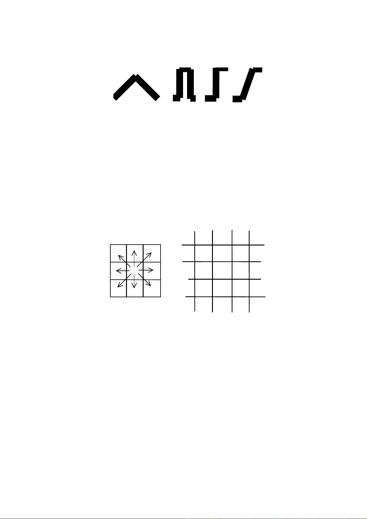
roof edge line edge step edge ramp edge
Figure 4.1 Different edge profiles.
There is an infinite number of edge orientations, widths and shapes (Figure 4.1). Some
edges are straight while others are curved with varying radii. There are many edge
detection techniques to go with all these edges, each having its own strengths. Some edge
detectors may work well in one application and perform poorly in others. Sometimes it
takes experimentation to determine what is the best edge detection technique for an
application.
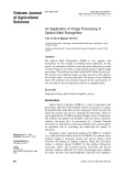
The simplest and quickest edge detectors determine the maximum value from a series of
pixel subtractions. The homogeneity operator subtracts each 8 surrounding pixels from the
center pixel of a 3 x 3 window as in Figure 4.2. The output of the operator is the maximum
of the absolute value of each difference.
homogenety operator image
11
11
11
11
11
12
16
16
13
15
new pixel = maximum{ 11−11 , 11−13 , 11−15 , 11−16 , 11−11 ,
11−16 , 11−12 , 11−11 } = 5
Figure 4.2 How the homogeneity operator works.
Similar to the homogeneity operator is the difference edge detector. It operates more
quickly because it requires four subtractions per pixel as opposed to the eight needed by
the homogeneity operator. The subtractions are upper left − lower right, middle left −
middle right, lower left − upper right, and top middle − bottom middle (Figure 4.3).

homogenety operator image
11
11
11
11
11
12
16
16
13
15
new pixel = maximum{ 11−11 , 13−12 , 15−16 , 11−16 } = 5
Figure 4.3 How the difference operator works.
4.2.1 First order derivative for edge detection
If we are looking for any horizontal edges it would seem sensible to calculate the
difference between one pixel value and the next pixel value, either up or down from the
first (called the crack difference), i.e. assuming top left origin
Hc = y_difference(x, y) = value(x, y) – value(x, y+1)
In effect this is equivalent to convolving the image with a 2 x 1 template
1
1
−
Likewise
Hr = X_difference(x, y) = value(x, y) – value(x – 1, y)
uses the template
–1 1
Hc and Hr are column and row detectors. Occasionally it is useful to plot both X_difference
and Y_difference, combining them to create the gradient magnitude (i.e. the strength of the
edge). Combining them by simply adding them could mean two edges canceling each
other out (one positive, one negative), so it is better to sum absolute values (ignoring the
sign) or sum the squares of them and then, possibly, take the square root of the result.
It is also to divide the Y_difference by the X_difference and identify a gradient direction
(the angle of the edge between the regions)
=−
y)ce(x,X_differen
y)ce(x,Y_differen
tanirectiongradient_d 1
The amplitude can be determine by computing the sum vector of Hc and Hr

)y,x(H)y,x(H)y,x(H 2
c
2
r+=
Sometimes for computational simplicity, the magnitude is computed as
)y,x(H)y,x(H)y,x(H cr +=
The edge orientation can be found by
( )
( )
y,xH
y,xH
tan
r
c
1−
=θ
In real image, the lines are rarely so well defined, more often the change between regions
is gradual and noisy.
The following image represents a typical read edge. A large template is needed to average
at the gradient over a number of pixels, rather than looking at two only
3444332100
2342334010
3333433100
3233430200
2420001000
3302000000
4.2.2 Sobel edge detection
The Sobel operator is more sensitive to diagonal edges than vertical and horizontal edges.
The Sobel 3 x 3 templates are normally given as
X-direction
121
000
121 −−−
Y-direction
101
202
101
−
−
−
Original image
3444332100
2342334010
3333433100
3233420200
2420001000
3302000000
absA + absB


![Giáo trình Ứng dụng AI trong dạy học môn Khoa học Tự nhiên [Chuẩn Nhất]](https://cdn.tailieu.vn/images/document/thumbnail/2026/20260526/vispacex_27/135x160/6141779796087.jpg)


![Ứng dụng trí tuệ nhân tạo: Tài liệu dẫn đầu [mới nhất]](https://cdn.tailieu.vn/images/document/thumbnail/2026/20260515/baobinh_011/135x160/9361778820542.jpg)


![Tài liệu Huấn luyện ChatGPT [Chuẩn Nhất]](https://cdn.tailieu.vn/images/document/thumbnail/2026/20260512/vispacex_27/135x160/453_tai-lieu-huan-luyen-chatgpt.jpg)
![Ứng dụng AI trong vận hành doanh nghiệp: Tài liệu [Mới nhất/Hướng dẫn chi tiết]](https://cdn.tailieu.vn/images/document/thumbnail/2026/20260512/vispacex_27/135x160/9141778583001.jpg)
![Ứng dụng AI và công cụ số trong công việc: Tài liệu [Mới nhất]](https://cdn.tailieu.vn/images/document/thumbnail/2026/20260512/vispacex_27/135x160/60101778665998.jpg)


%20--%3e%3cdefs%3e%3cstyle%3e%20.st0%20{%20fill:%20%23fff;%20}%20.st1%20{%20fill:%20%237800fa;%20}%20%3c/style%3e%3c/defs%3e%3cpath%20class='st1'%20d='M117.78,12.18H43.11c2.9,3.47,4.65,7.94,4.65,12.82,0,5.6-2.3,10.66-6.01,14.29h76.02l7.22-13.56-7.22-13.56Z'/%3e%3cg%3e%3cpath%20class='st0'%20d='M53.58,26.17h-.59v-1.46h.59v-4.96h2.83c1.78,0,2.67.94,2.67,2.82v5.76c0,1.87-.89,2.81-2.67,2.81h-2.83v-4.96ZM55.36,21.37v3.34h1.1v1.46h-1.1v3.34h1.01c.61,0,.91-.37.91-1.1v-5.93c0-.74-.3-1.1-.91-1.1h-1.01Z'/%3e%3cpath%20class='st0'%20d='M65.99,31.14h-1.8l-.31-2.07h-2.19l-.31,2.07h-1.64l1.82-11.39h2.62l1.82,11.39ZM65.28,18.04c-.25.46-.51.77-.75.94-.21.15-.47.22-.79.22-.26,0-.57-.07-.92-.22l-.38-.15c-.14-.05-.26-.07-.37-.07-.3,0-.53.18-.71.54l-.91-.68c.25-.46.51-.77.75-.94.21-.14.48-.21.79-.21.26,0,.57.07.92.21l.38.15c.14.05.26.07.37.07.3,0,.53-.18.71-.54l.91.68ZM61.91,27.52h1.73l-.87-5.76-.87,5.76Z'/%3e%3cpath%20class='st0'%20d='M74.53,26.89v1.52c0,1.91-.89,2.86-2.67,2.86s-2.67-.95-2.67-2.86v-5.93c0-1.91.89-2.86,2.67-2.86s2.67.95,2.67,2.86v1.11h-1.69v-1.22c0-.75-.31-1.12-.93-1.12s-.93.37-.93,1.12v6.15c0,.74.31,1.11.93,1.11s.93-.37.93-1.11v-1.63h1.69Z'/%3e%3cpath%20class='st0'%20d='M81.4,31.14h-1.8l-.31-2.07h-2.19l-.31,2.07h-1.64l1.82-11.39h2.62l1.82,11.39ZM75.9,19.2l1.52-1.91h1.71l1.51,1.91h-1.61l-.76-.95-.75.95h-1.61ZM77.32,27.52h1.73l-.87-5.76-.87,5.76ZM83.1,15.99l-1.76,1.91h-1.26l1.17-1.91h1.86Z'/%3e%3cpath%20class='st0'%20d='M84.86,19.75c1.78,0,2.67.94,2.67,2.82v1.48c0,1.87-.89,2.81-2.67,2.81h-.85v4.28h-1.79v-11.39h2.64ZM84.01,21.37v3.86h.85c.58,0,.87-.36.87-1.08v-1.71c0-.71-.29-1.07-.87-1.07h-.85Z'/%3e%3cpath%20class='st0'%20d='M93.51,19.75c1.78,0,2.67.94,2.67,2.82v1.48c0,1.87-.89,2.81-2.67,2.81h-.85v4.28h-1.79v-11.39h2.64ZM92.66,21.37v3.86h.85c.58,0,.87-.36.87-1.08v-1.71c0-.71-.29-1.07-.87-1.07h-.85Z'/%3e%3cpath%20class='st0'%20d='M98.8,31.14h-1.79v-11.39h1.79v4.88h2.03v-4.88h1.83v11.39h-1.83v-4.88h-2.03v4.88Z'/%3e%3cpath%20class='st0'%20d='M105.36,24.55h2.46v1.62h-2.46v3.34h3.09v1.63h-4.88v-11.39h4.88v1.63h-3.09v3.18ZM108.17,17.29l-1.76,1.91h-1.26l1.17-1.91h1.86Z'/%3e%3cpath%20class='st0'%20d='M112.2,19.75c1.78,0,2.67.94,2.67,2.82v1.48c0,1.87-.89,2.81-2.67,2.81h-.85v4.28h-1.79v-11.39h2.64ZM111.35,21.37v3.86h.85c.58,0,.87-.36.87-1.08v-1.71c0-.71-.29-1.07-.87-1.07h-.85Z'/%3e%3c/g%3e%3ccircle%20class='st1'%20cx='25'%20cy='25'%20r='20'/%3e%3cpath%20class='st0'%20d='M32.78,19.27c2.92,0,4.43,2.55,5.28,5.33l.71,2.17c.14.38-.33.75-.71.75h-5.61c.19-.33.24-.71.09-1.08l-.75-2.45c-.43-1.32-.99-2.64-1.79-3.77.75-.57,1.65-.94,2.78-.94h0ZM25,18.38c3.25,0,4.9,2.78,5.89,5.89l.76,2.45c.14.42-.33.8-.8.8h-11.69c-.42,0-.94-.38-.8-.8l.75-2.45c.99-3.11,2.64-5.89,5.89-5.89h0ZM25,11.35c1.74,0,3.11,1.37,3.11,3.11s-1.37,3.11-3.11,3.11-3.11-1.41-3.11-3.11,1.41-3.11,3.11-3.11h0ZM17.27,19.27c1.08,0,1.98.38,2.73.94-.8,1.13-1.37,2.45-1.74,3.77l-.8,2.45c-.14.38-.05.75.09,1.08h-5.56c-.42,0-.9-.38-.75-.75l.71-2.17c.9-2.78,2.41-5.33,5.33-5.33h0ZM17.27,12.91c1.51,0,2.78,1.27,2.78,2.83s-1.27,2.83-2.78,2.83-2.83-1.27-2.83-2.83,1.27-2.83,2.83-2.83h0ZM32.78,12.91c1.56,0,2.78,1.27,2.78,2.83s-1.23,2.83-2.78,2.83-2.83-1.27-2.83-2.83,1.27-2.83,2.83-2.83h0ZM27.07,28.56v.09c0,.57-.24,1.08-.61,1.46h0v.05c-.38.33-.9.57-1.46.57s-1.08-.24-1.46-.61h0c-.38-.38-.61-.9-.61-1.46v-.09h1.41v.09c0,.19.05.38.19.47v.05c.09.09.28.19.47.19s.38-.09.47-.19v-.05c.14-.09.24-.28.24-.47t-.05-.09h1.41ZM30.99,28.56v.09c0,1.65-.66,3.16-1.74,4.24-1.08,1.08-2.59,1.79-4.24,1.79s-3.16-.71-4.24-1.79l-.05-.05c-1.04-1.08-1.7-2.55-1.7-4.2v-.09h1.41v.09c0,1.27.47,2.4,1.27,3.25h.05c.85.85,1.98,1.37,3.25,1.37s2.4-.52,3.25-1.37c.85-.8,1.37-1.98,1.37-3.25v-.09h1.37ZM34.99,28.56v.09c0,2.78-1.13,5.28-2.92,7.07-1.79,1.79-4.29,2.92-7.07,2.92s-5.23-1.13-7.07-2.92c-1.79-1.79-2.92-4.29-2.92-7.07v-.09h1.41v.09c0,2.4.94,4.53,2.5,6.08,1.56,1.56,3.72,2.5,6.08,2.5s4.52-.94,6.08-2.5c1.56-1.56,2.5-3.68,2.5-6.08v-.09h1.41Z'/%3e%3c/svg%3e)