0 50 100
−2
0
2
V1(n)
n
(a)
(b)
(c)(f)
(e)
(d)
0 50 100
−2
0
2
−0.05
0
0.05
V2(n)
VT(n)
n
0204060
n
−150
−130
−110
−90
−70
−50
020
k
k
40 60
−150
−130
−110
−90
−70
−50
0204060
VT2(k)
VT(k)
VN2(k)
VN(k)
dB
dB
N := 128 n := 0, 1.. N− 1k := 0, 1.. N− 1
V1(n) := sin V2(n) := cos
2⋅π⋅ ⋅1
n
N2⋅π⋅ ⋅1− 0.1⋅ (rnd(1) − .5)
n
N
VT(n) := V1(n)⋅ V2(n)− 0.5 sin 2⋅π⋅ ⋅2
n
N
VT(k) := 20⋅log
VT1(k) := 0.25 VT(k− 1) + 0.5 VT(k)+ 0.25 VT(k+ 1)
VT2(k) := 0.25 VT1(k − 1) + 0.5 VT1(k)+ 0.25 VT1(k+ 1)
VN1(k) := 0.25 VN(k− 1) + 0.5 VN(k)+ 0.25 VN(k+ 1)
VN2(k) := 0.25 VN1(k− 1) + 0.5 VN1(k)+ 0.25 VN1(k+ 1)
VN(k) := VT(k)− 20⋅log(1+k2)
∑
N−1
n= 0
1
N
k
N
VT(n)⋅exp −j⋅2⋅π⋅ ⋅n
⋅
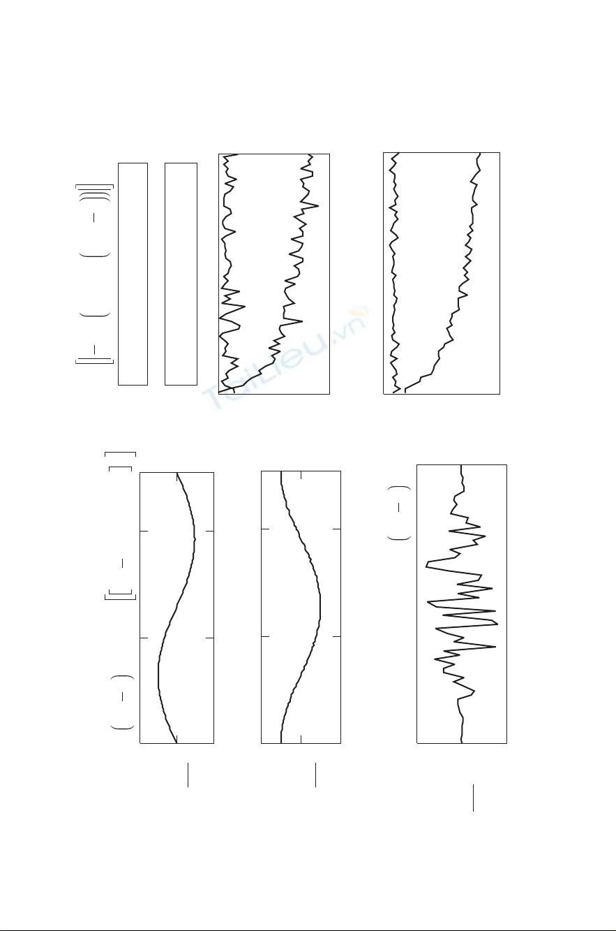
Figure 7-4 Phase noise on a test signal sine wave.
126

THE POWER SPECTRUM 127
At the upper left is a noise-free discrete sine wave V1(n) at frequency
f=1.0, amplitude 1.0, in 128 positions of (n). A discrete cosine wave
V2(n), amplitude 1.0 at the same frequency, has some phase noise added,
0.1·[rnd(1) −0.5]. The rnd(1) function creates a random number from
0to+1 at each position of (n). The value 0.5 is subtracted, so the
random number is then between −0.5 and +0.5. The index of the phase
modulation is 0.1.
(a) The plot of the noise-free sine wave.
(b) The plot of the cosine wave with the noise just barely visible.
(c) We now multiply the sine wave and the cosine wave. This mul-
tiplication produces the baseband phase noise output VT (n) and a
sine wave of amplitude 0.5 at twice the frequency of the two input
waves. We subtract this unwanted wave so that only the phase noise
is visible in part (c). This is equivalent to a lowpass Þlter that rejects
the times 2 frequency. Note the vertical scale in the graph of part
(c) that shows the phase noise greatly ampliÞed.
(d) We next use the DFT to get the noise spectrum VT (k) in dB format.
At this point we also perform two 3-point smoothing operations on
VT (k), Þrst to get VT 1(k) and then to get VT 2(k). This operation
smoothes the spectrum of VT (k)sothatVT (k) in the graph in
part (e) is smoothed to VT 2(k) in the graph in part (f). This is
postdetection Þltering that is used in spectrum analyzers and many
other applications to get a smoother appearance and reduce noise
peaks; it improves “readability” of the noise shelf value.
(e) Also in part (d) we perform lowpass Þltering [−20 log(1 +k2)]
(a Butterworth lowpass Þlter) to get VN (k). This result is also
smoothed two times and the comparison of VN (k)andVN 2(k)is
seen in the graphs of parts (e) and (f).
(f) Note that in parts (e) and (f) the upper level of the phase noise plot
VT (k)andVT 2(k)is>53 dB below the 0-dB reference level of the
test signal V2at frequency k=1. This is called the relative noise
shelf for the noisy test signal that we used. It is usually expressed
as a dBc number (dB below the carrier, in this case, >53 dBc). This
noise shelf is of great signiÞcance in equipment design. It deÞnes
the ability to reject interference to and from closely adjacent signals

128 DISCRETE-SIGNAL ANALYSIS AND DESIGN
and also to analyze unwanted phase disturbances on input signals.
The lowpass Þlter to get VN 2(k) greatly improves phase noise, but
only at frequencies somewhat removed from the signal frequency.
Still, it is very important that wideband phase noise interference is
greatly reduced.
In conclusion, there are many advanced applications of the cross power
spectrum that we cannot cover in this book but that can be explored using
various search engines and texts.
REFERENCES
Carlson, A., 1986, Communication Systems, 3rd ed., McGraw-Hill, New York.
Dorf, R. C., and R. H. Bishop, 2005, Modern Control Systems, 10th ed., Prentice
Hall, Englewood Cliffs, NJ.
Gonzalez, G., 1997, Microwave Transistor AmpliÞer Analysis and Design, Pren-
tice Hall, Upper Saddle River, NJ.
Oppenheim, A. V., and R. W. Schafer, 1999, Discrete-Time Signal Processing,
2nd ed., Prentice-Hall, Upper Saddle River, NJ, p. 189.
Papoulis, A., 1965, Probability, Random Variables, and Stochastic Processes,
McGraw-Hill, New York.
Sabin, W. E., 1988, Envelope detection and noise Þgure measurement, RF
Design, Nov., p. 29.
Sabin, W. E., and E. O. Schoenike, 1998, HF Radio Systems and Circuits,
SciTech, Mendham, NJ.
Schwartz, M., 1980, Information Transmission, Modulation and Noise, 3rd ed.,
McGraw-Hill, New York, Chap. 5.
Shearer, J. L., A. T. Murphy, and H. H. Richardson, 1971, Introduction to System
Dynamics, Addison-Wesley, Reading, MA.

8
The Hilbert
Transform D. Hilbert 1862-1943
This Þnal chapter considers a valuable resource, the Hilbert transform
(HT), which is used in signal-processing systems to achieve certain prop-
erties in the time domain and the frequency domain. The DFT, IDFT,
FFT, and Hilbert transform work quite well together with discrete signals
if certain problem areas to be discussed are handled correctly.
Example of the Hilbert Transform
Figure 8-1 shows a two-sided square wave x(n) time sequence, and
we will walk through the creation of an HT for this wave. Design the
two-sided square-wave time sequence using N=128. The value at n=0
is zero, which provides a sloping leading edge for better plot results. Val-
ues from 1 to N/2 −1=+1.0. Set the N/2 position to zero, which has
been found to be important for successful execution of the HT because
N/2 is a special location that can cause problems because of its small
but non-zero value. Values from N/2 +1to N −1=−1. At Nthe wave
returns to zero.
(a) Plot the two-sided square wave from n=0toN−1.
Discrete-Signal Analysis and Design, By William E. Sabin
Copyright 2008 John Wiley & Sons, Inc.
129

130 DISCRETE-SIGNAL ANALYSIS AND DESIGN
(b) Execute the DFT to get X(k), the two-sided, positive-frequency Þrst-
half and negative-frequency second-half phasor spectrum. This spec-
trum is a set of sine waves as shown in Fig. 2-2c. Each sine wave
consists of two imaginary components.
(c) Multiply the Þrst-half positive-frequency X(k) values by –jto get
a90
◦phase lag. Multiply the second-half negative-frequency X(k)
values by +jtogeta90
◦phase lead. As in step (a), be sure to set the
N/2 value to zero. This value can sometimes confuse the computer
unless it is forced to zero. This step (c) is the ideal Hilbert transform.
(d) Part (d) of the graph shows the two-sided spectrum XH (k) after the
phase shifts of part (c). This spectrum is a set of negative cosine
waves as shown in Fig. 2-2b. Each cosine wave consists of two real
negative components, one at +kand one at N−k.
(e) Use the IDFT to get the two-sided xh(n) time response. Note that
xh(n) is a sequence of real numbers because x(n) is real.
(f) The original square wave and its HT are both shown in the graph.
Note the large peaks at the ends and in the center. These peaks are
characteristic of the HT of an almost square wave. The perfect square
wave would have inÞnite (very undesirable) peaks.
(g) Calculate two 3-point smoothing sequences described in Chapter 4
for the sequence in part (f). This smoothing is equivalent to a lowpass
Þlter, or at radio frequencies to a narrow band-pass Þlter.
(h) Plot the Þnal result. The sharp peaks have been reduced by about
2 dB. Further smoothing is usually required in narrowband circuit
design applications, as we will see later.
The three peaks in part (f) are usually a problem in any peak-power-
limited system (which is almost always the practical situation). The
smoothing in part (h) thus becomes important. Despite the peaks, the
rms voltage in part (f) is the same for both of the waveforms in that
diagram (nothing is lost).
For problems of this type, the calculation effort becomes extensive,
and the use of the FFT algorithm, with its greater speed, would ordinarily
be preferred. The methods of the Mathcad FFT and IFFT functions are
described in the User Guide and especially in the online Help. In this


![Ngân hàng đề thi trắc nghiệm Kiến trúc máy tính [mới nhất]](https://cdn.tailieu.vn/images/document/thumbnail/2026/20260514/hoahongxanh0906/135x160/49281779160279.jpg)


%20--%3e%3cdefs%3e%3cstyle%3e%20.st0%20{%20fill:%20%23fff;%20}%20.st1%20{%20fill:%20%237800fa;%20}%20%3c/style%3e%3c/defs%3e%3cpath%20class='st1'%20d='M117.78,12.18H43.11c2.9,3.47,4.65,7.94,4.65,12.82,0,5.6-2.3,10.66-6.01,14.29h76.02l7.22-13.56-7.22-13.56Z'/%3e%3cg%3e%3cpath%20class='st0'%20d='M53.58,26.17h-.59v-1.46h.59v-4.96h2.83c1.78,0,2.67.94,2.67,2.82v5.76c0,1.87-.89,2.81-2.67,2.81h-2.83v-4.96ZM55.36,21.37v3.34h1.1v1.46h-1.1v3.34h1.01c.61,0,.91-.37.91-1.1v-5.93c0-.74-.3-1.1-.91-1.1h-1.01Z'/%3e%3cpath%20class='st0'%20d='M65.99,31.14h-1.8l-.31-2.07h-2.19l-.31,2.07h-1.64l1.82-11.39h2.62l1.82,11.39ZM65.28,18.04c-.25.46-.51.77-.75.94-.21.15-.47.22-.79.22-.26,0-.57-.07-.92-.22l-.38-.15c-.14-.05-.26-.07-.37-.07-.3,0-.53.18-.71.54l-.91-.68c.25-.46.51-.77.75-.94.21-.14.48-.21.79-.21.26,0,.57.07.92.21l.38.15c.14.05.26.07.37.07.3,0,.53-.18.71-.54l.91.68ZM61.91,27.52h1.73l-.87-5.76-.87,5.76Z'/%3e%3cpath%20class='st0'%20d='M74.53,26.89v1.52c0,1.91-.89,2.86-2.67,2.86s-2.67-.95-2.67-2.86v-5.93c0-1.91.89-2.86,2.67-2.86s2.67.95,2.67,2.86v1.11h-1.69v-1.22c0-.75-.31-1.12-.93-1.12s-.93.37-.93,1.12v6.15c0,.74.31,1.11.93,1.11s.93-.37.93-1.11v-1.63h1.69Z'/%3e%3cpath%20class='st0'%20d='M81.4,31.14h-1.8l-.31-2.07h-2.19l-.31,2.07h-1.64l1.82-11.39h2.62l1.82,11.39ZM75.9,19.2l1.52-1.91h1.71l1.51,1.91h-1.61l-.76-.95-.75.95h-1.61ZM77.32,27.52h1.73l-.87-5.76-.87,5.76ZM83.1,15.99l-1.76,1.91h-1.26l1.17-1.91h1.86Z'/%3e%3cpath%20class='st0'%20d='M84.86,19.75c1.78,0,2.67.94,2.67,2.82v1.48c0,1.87-.89,2.81-2.67,2.81h-.85v4.28h-1.79v-11.39h2.64ZM84.01,21.37v3.86h.85c.58,0,.87-.36.87-1.08v-1.71c0-.71-.29-1.07-.87-1.07h-.85Z'/%3e%3cpath%20class='st0'%20d='M93.51,19.75c1.78,0,2.67.94,2.67,2.82v1.48c0,1.87-.89,2.81-2.67,2.81h-.85v4.28h-1.79v-11.39h2.64ZM92.66,21.37v3.86h.85c.58,0,.87-.36.87-1.08v-1.71c0-.71-.29-1.07-.87-1.07h-.85Z'/%3e%3cpath%20class='st0'%20d='M98.8,31.14h-1.79v-11.39h1.79v4.88h2.03v-4.88h1.83v11.39h-1.83v-4.88h-2.03v4.88Z'/%3e%3cpath%20class='st0'%20d='M105.36,24.55h2.46v1.62h-2.46v3.34h3.09v1.63h-4.88v-11.39h4.88v1.63h-3.09v3.18ZM108.17,17.29l-1.76,1.91h-1.26l1.17-1.91h1.86Z'/%3e%3cpath%20class='st0'%20d='M112.2,19.75c1.78,0,2.67.94,2.67,2.82v1.48c0,1.87-.89,2.81-2.67,2.81h-.85v4.28h-1.79v-11.39h2.64ZM111.35,21.37v3.86h.85c.58,0,.87-.36.87-1.08v-1.71c0-.71-.29-1.07-.87-1.07h-.85Z'/%3e%3c/g%3e%3ccircle%20class='st1'%20cx='25'%20cy='25'%20r='20'/%3e%3cpath%20class='st0'%20d='M32.78,19.27c2.92,0,4.43,2.55,5.28,5.33l.71,2.17c.14.38-.33.75-.71.75h-5.61c.19-.33.24-.71.09-1.08l-.75-2.45c-.43-1.32-.99-2.64-1.79-3.77.75-.57,1.65-.94,2.78-.94h0ZM25,18.38c3.25,0,4.9,2.78,5.89,5.89l.76,2.45c.14.42-.33.8-.8.8h-11.69c-.42,0-.94-.38-.8-.8l.75-2.45c.99-3.11,2.64-5.89,5.89-5.89h0ZM25,11.35c1.74,0,3.11,1.37,3.11,3.11s-1.37,3.11-3.11,3.11-3.11-1.41-3.11-3.11,1.41-3.11,3.11-3.11h0ZM17.27,19.27c1.08,0,1.98.38,2.73.94-.8,1.13-1.37,2.45-1.74,3.77l-.8,2.45c-.14.38-.05.75.09,1.08h-5.56c-.42,0-.9-.38-.75-.75l.71-2.17c.9-2.78,2.41-5.33,5.33-5.33h0ZM17.27,12.91c1.51,0,2.78,1.27,2.78,2.83s-1.27,2.83-2.78,2.83-2.83-1.27-2.83-2.83,1.27-2.83,2.83-2.83h0ZM32.78,12.91c1.56,0,2.78,1.27,2.78,2.83s-1.23,2.83-2.78,2.83-2.83-1.27-2.83-2.83,1.27-2.83,2.83-2.83h0ZM27.07,28.56v.09c0,.57-.24,1.08-.61,1.46h0v.05c-.38.33-.9.57-1.46.57s-1.08-.24-1.46-.61h0c-.38-.38-.61-.9-.61-1.46v-.09h1.41v.09c0,.19.05.38.19.47v.05c.09.09.28.19.47.19s.38-.09.47-.19v-.05c.14-.09.24-.28.24-.47t-.05-.09h1.41ZM30.99,28.56v.09c0,1.65-.66,3.16-1.74,4.24-1.08,1.08-2.59,1.79-4.24,1.79s-3.16-.71-4.24-1.79l-.05-.05c-1.04-1.08-1.7-2.55-1.7-4.2v-.09h1.41v.09c0,1.27.47,2.4,1.27,3.25h.05c.85.85,1.98,1.37,3.25,1.37s2.4-.52,3.25-1.37c.85-.8,1.37-1.98,1.37-3.25v-.09h1.37ZM34.99,28.56v.09c0,2.78-1.13,5.28-2.92,7.07-1.79,1.79-4.29,2.92-7.07,2.92s-5.23-1.13-7.07-2.92c-1.79-1.79-2.92-4.29-2.92-7.07v-.09h1.41v.09c0,2.4.94,4.53,2.5,6.08,1.56,1.56,3.72,2.5,6.08,2.5s4.52-.94,6.08-2.5c1.56-1.56,2.5-3.68,2.5-6.08v-.09h1.41Z'/%3e%3c/svg%3e)