The Economic Theory of Annuities by Eytan Sheshinski_2

Chia sẻ: Thao Thao | Ngày: | Loại File: PDF | Số trang:19

Thêm vào BST

Báo xấu

51
lượt xem 11
download

Download Vui lòng tải xuống để xem tài liệu đầy đủ

Tham khảo tài liệu 'the economic theory of annuities by eytan sheshinski_2', tài chính - ngân hàng, ngân hàng - tín dụng phục vụ nhu cầu học tập, nghiên cứu và làm việc hiệu quả

Chủ đề:

Bình luận(0) Đăng nhập để gửi bình luận!

Lưu

Nội dung Text: The Economic Theory of Annuities by Eytan Sheshinski_2

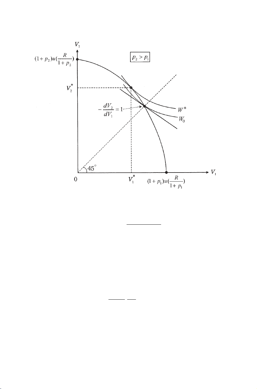
August 18, 2007 Time: 11:06am chapter13.tex Utilitarian Pricing of Annuities • 111 Figure 13.1. First-best allocation of utilities. while R ∗ Vh = (1 + ph ) u . H + ph ) h=1 (1 Thus, the utilitarian ﬁrst best has inequality in expected utilities but may have equality in consumption levels (Arrow, 1992). This result is similar to Mirrlees’ (1971) optimum income tax model where individuals differ in productivity.2 The ﬁrst best allocation pro- vides higher (expected) utility to those with a higher capacity to produce utility. In the appendix to this chapter it is shown that ∗ 1 + pn ∂ ch 0> > −1, (13.7) ∗ ch ∂ ph ∗ while ∂ ch /∂ p j 0, for j = h, h, j = 1, 2, . . . , n. 2 In Mirrlees’ model with additive utilities, the ﬁrst best has all individuals with equal consumption, and those with higher productivity, having a lower disutility for generating a given income, are assigned to work more and hence have a lower utility.
August 18, 2007 Time: 11:06am chapter13.tex 112 • Chapter 13 Concavity of u and (13.7) imply ∗ ∂ c∗ ∂ Vh ∗ = u(ch ) + (1 + pn )u (cn ) h > 0, (13.8) ∂ ph ∂ pn ∗ while ∂ Vh /∂ p j 0, j = h, j = 1, 2, . . . , H.3 Thus, with the given total resources, an increase in one individual’s survival probability decreases his or her optimum consumption, but the positive effect of higher survival probability on expected utility dominates. The effect on the welfare of other individuals facing only resource redistribution depends on the shape of the social welfare function. 13.2 Competitive Annuity Market with Full Information In a competitive market with full information on the survival proba- bilities of individuals and a zero rate of interest, the price of a unit of second-period consumption, c2h , is equal to the survival probability of each annuitant. Individuals maximize expected utility subject to a budget constraint c1h + ph c2h = yh h = 1, 2, . . . , H, (13.9) where yh is the given income of individual h. Demands for ﬁrst- and second-period consumption (annuities), c1h and c2h , are given by c1h = c2h = ch = yh /(1 + ph ). The ﬁrst-best allocation can be supported by a competitive annuity market accompanied by an optimum income allocation. Equating con- ∗ sumption levels under competition, ch , to the optimum levels, ch ( p), ∗ yields unique income levels, yh = (1 + ph )ch (p), that support the ﬁrst-best allocation. In particular, with an additive W, all individuals consume the same amount: R ∗ ch = , H + ph ) h=1 (1 hence 1 + ph yh = R. (13.10) H + ph ) h=1 (1 3 In the extreme case when W = min[ V , V , . . . , V ], optimum expected utilities, H 1 2 ∗ ∗ ∗ Vh = (1 + ph )u(ch ), are equal, and hence optimum consumption, ch , strictly decreases with ph (and increases with p j , j = h).
August 18, 2007 Time: 11:06am chapter13.tex Utilitarian Pricing of Annuities • 113 13.3 Second-best Optimum Pricing of Annuities Governments do not engage, for well-known reasons, in unconstrained lump-sum redistributions of incomes. In contrast, most annuities are supplied directly by government-run social security systems and taxes/subsidies can, if so desired, be applied to the prices of annuities offered by private pension funds. These prices can be used by govern- ments to improve social welfare. Although deviations from actuarially fair prices entail distortions (i.e., efﬁciency losses), distributional im- provements may outweigh the costs.4 Suppose that individual h purchases annuities at a price of qh . With an income yh , his or her budget constraint is c1h + qh c2h = yh , h = 1, 2 . . . , H. (13.11) Maximization of (13.2) subject to (13.11) yields demands ci h = ci h (qh , ph , yh ), i = 1, 2, and h = 1, 2, . . . , H. Maximized expected utility, Vh , is Vh (qh , ph , yh ) = u(c1h ) + ph u(c2h ). Assume that no outside resources are available for the annuity market, hence total subsidies/taxes must equal zero, H (qh − ph )c2h = 0. (13.12) h=1 Maximization of W(V1 , V2 , . . . , VH ) with respect to prices (q1 , . . . , qH ) subject to (13.12) yields the ﬁrst-order condition ∂ W ∂ Vh ∂ c2h + λ c2h + (qh − ph ) = 0, h = 1, 2, . . . , H, (13.13) ∂ qh ∂ Vh dqh where λ > 0 is the shadow price of constraint (13.12). In elasticity form, using Roy’s identity (∂ Vh /∂ qh = −(∂ Vh /∂ yh )c2h ), (13.13) can be written qh − ph θh =, (13.14) εh qh where ε h = −(qh /c2h )(∂ c2h /dqh ) is the price elasticity of second-period consumption of individual h and 1 ∂ W ∂ Vh θh = 1 − λ ∂ Vh ∂ yh 4 In practice, of course, prices do not vary individually. Rather, individuals with similar survival probabilities are grouped into risk classes, and annuity prices and taxes/subsidies vary across these classes.
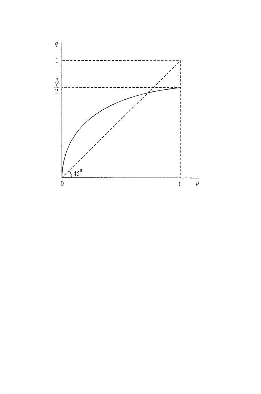
August 18, 2007 Time: 11:06am chapter13.tex 114 • Chapter 13 is the net social value of a marginal transfer to individual h through the optimum pricing scheme. Equation (13.14) is a variant of the well-known inverse elasticity optimum tax formula, which combines equity (θ h ) and efﬁciency (1/ε h ) considerations. The implication of (13.14) for the optimum pricing of annuities depends on the welfare function, W, and on the joint distribution of incomes, ( y1 , . . . , yH ), and probabilities, ( p1 , . . . , pH ). To obtain some concrete examples, let W be the sum of expected utilities. Then ∂ W/∂ Vh = 1, h = 1, 2, . . . , H. Assume further that Vh = ln c1h + ph ln c2h . In this case, demands are yh yh ph c1h = , c2h = , (13.15) 1 + ph 1 + ph qh and yh ph Vh = (1 + ph ) ln + ph ln . (13.16) 1 + ph qh Conditions (13.14) and (13.12) now yield the solution βh qh = φ , (13.17) H h=1 β h where H ph yh φ= ph > 0 and βh = > 0. 1 + ph h=1 Consider two special cases of (13.17): (a) Equal incomes: ( yh = y = R/ H; h = 1, 2, . . . , H) ¯ Condition (13.17) now becomes qh = φ ( ph /(1 + ph )), where H h=1 ph ¯ φ= (>1). (13.18) ph H h=1 1 + ph It is seen (ﬁgure 13.2) that optimum pricing involves subsidization (taxation) of individuals with high (low) survival probabilities.5 ¯ In ﬁgure 13.2, it can be shown that φ/2 < 1. 5
August 18, 2007 Time: 11:06am chapter13.tex Utilitarian Pricing of Annuities • 115 Figure 13.2. Optimum annuity pricing in a full-information equilibrium. (b) yh = y(1 + ph ) This, one recalls, is the ﬁrst-best utilitarian income distribution, and since all price elasticities are equal to unity, we see from (13.17), as expected, that qh = ph ; that is efﬁciency prices are optimal. More generally, it is seen from (13.17) that a higher correlation between incomes, yh , and survival probabilities, ph , decreases—and possibly eliminates—the subsidization of high-survival individuals. In contrast, a negative correlation between incomes and survival probabilities (as, presumably, in the female/male case) leads to subsidies for high- survival individuals, possibly to the commonly observed uniform pricing rule.
August 18, 2007 Time: 11:06am chapter13.tex Appendix Let H = 2. The extension to H > 2 is immediate. The ﬁrst-order conditions for maximization of (13.1) subject to (13.3) are ∗ ∗ ∗ W1 (U1 , U2 )u (c1 ) − λ = 0, ∗ ∗ ∗ W2 (U1 , U2 )u (c2 ) − λ = 0, ∗ ∗ R − (1 + p1 )c1 − (1 + p2 )c2 = 0, (13A.1) ∗ ∗ where Uh = (1 + ph )u(ch ), h = 1, 2. Totally differentiating (13A.1) with respect to p1 yields ∗ (1 + p1 ) ∂ c1 1 ∗ = (1 + p1 )(1 + p2 ) (W11 u (c1 )2 ∗ ∂ p1 c1 c ∗ u (c ∗ ) ∗ ∗ ∗ ∗ −W12 u (c1 )u (c2 )) 1 ∗ 1 − W12 u (c1 )u (c2 ) u(c1 ) ∗ ∗ +W22 u (c2 )2 + W2 u (c2 )(1 + p1 ) , (13A.2) where (using (13A.1)) (1 + p1 )(1 + p2 )λ2 =− [W11 W2 − 2W12 W1 W2 + W22 W1 ] 2 2 22 W1 W2 ∗ ∗ −(1 + p1 )W2 u (c2 ) − (1 + p2 )W1 u (c1 ). (13A.3) Strict quasi-concavity of W implies that > 0. ∗ ∗ ∗ Since 0 < c1 u (c1 )/u(c1 ) < 1, inserting again (13A.1) into (13A.2), we obtain ∗ ∗ (1 + p1 ) ∂ c1 0> > −1, (13A.4) ∗ ∂ p1 c1 as stated in the text.
August 18, 2007 Time: 11:06am chapter13.tex Chapter 13 • 117 Differentiating (13A.1) with respect to p2 , ∗ ∗ (1 + p2 ) ∂ c1 1 u(c2 ) ∗ ∗ = (1 + p1 )(1 + p2 )[W11 u (c1 )2 − W22 u (c2 )2 ∗ ∗ ∗ ∂ p2 c2 c2 u (c2) ∗ u(c2 ) ∗ ∗ ∗ ∗ ∗ −W12 u (c1 )u(c2 ) −W12 u (c1 )u(c2 ) −W1 u (c1 ) . ∗ ∗ c2 u(c2 ) (13A.5) The ﬁrst term on the right hand side is negative, and the second is ∗ positive, hence the sign of ∂ c1 /∂ p2 cannot be established in general.
August 18, 2007 Time: 10:43am chapter12.tex C H A P T E R 12 Annuities, Longevity, and Aggregate Savings 12.1 Changes in Longevity and Aggregate Savings In chapter 5 it was shown that when an increase in survival probabilities is tilted toward older ages, then individuals save more during their working years in order to support a longer retirement. Chosen retirement ages also rise with longevity, but this was shown to compensate only partially for the need to decrease consumption. In this chapter we shift the emphasis from individual savings to aggregate savings. When aggregating the response of individuals to changes in longevity, one has to take into account that over time these changes affect the population’s age density function (this is called the age composition effect in contrast to the response of individuals, called the behavioral effect). The direction of the change in this function reﬂects two opposite effects. First, an increase in survival rates increases the size of all age cohorts, particularly in older ages. Second, for given age-speciﬁc birthrates, an increase in survival probabilities raises the population’s long-run growth rate which, in turn, increases the relative weight of younger cohorts in the population’s age density function. Since older ages are typically retirees who are dissavers, while younger ages are savers, the ﬁrst effect tends to reduce aggregate savings while the second effect tends to raise their level. We shall provide conditions that ensure that the latter effect is dominant. The dynamics of demographic processes generated by a change in survival probabilities is quite complex. There exists, however, a well-developed theory on the dependence of steady-state age density distributions on the underlying parameters (e.g., Coale, 1972). The analysis below builds on this theory. The relation between life expectancy and aggregate savings has been explored empirically in many studies (e.g., Kinugasa and Mason, 2007; Miles, 1999; Deaton and Paxson, 2000; and Lee, Mason, and Miller, 2001). All these articles ﬁnd a positive correlation between life expectancy and aggregate savings. Since these studies have no explicit aggregation of individuals’ response functions, they do not attempt to identify separately the direction and size of the behavioral effect and the age composition effect. Furthermore, it is shown below that a
August 18, 2007 Time: 10:43am chapter12.tex 98 • Chapter 12 change in life expectancy is, in itself, inadequate to predict individu- als’ response and hence aggregate changes. This response depends on more speciﬁc assumptions about the age-related changes in survival probabilities. The existence of a competitive annuity market is crucial for individual decisions on savings and retirement. In the absence of this market, these decisions have to take into account the existence of unintended bequests, that is, assets left at death because individuals do not want to outlive their resources. Under these circumstances, an uncertain lifetime generates a random distribution of bequests that become initial endowments of a subsequent generation. Thus, analysis of the long-term effects of changes in longevity has to focus on the (ergodic) evolution of the distribution of these bequests and endowments. Section 12.6 provides an example of such an analysis. 12.2 Longevity and Individual Savings In chapter 4 it was shown that individuals’ optimum consumption, c∗ , is given by R∗ 0 w (z) F (z, α ) dz ∗ c =− (12.1) ¯ z and optimum retirement age, R∗ , is determined by the condition u (c∗ )w ( R∗ ) − e( R∗ ) = 0, (12.2) ∞ where z(α ) = 0 F (z, α ) dz is expected lifetime. A decrease in α is taken ¯ to increase survival probabilities, ∂ F (z, α )/∂α < 0, for all z. Recall that µ(z, α ) is the proportional change in the survival function at age z due to a small change in α : ∂ F (z, α ) 1 µ(z, α ) = (< 0). F (z, α ) ∂α Differentiating (12.1) and (12.2) totally with respect to α , it was shown that when µ(z, α ) decreases with z (equivalently, that a decrease in α decreases the hazard rate), then dc∗ /dα > 0 and dR∗ /dα < 0. 12.3 Longevity and Aggregate Savings Suppose that the population grows at a constant rate, g . The steady- state age density function of the population, denoted h(z, α, g ), is
August 18, 2007 Time: 10:43am chapter12.tex Annuities and Aggregate Savings • 99 given by1 h(z, α, g ) = me−gz F (z, α ), (12.3) ∞ where m = 1/ 0 e−gz F (z, α ) dz is the birthrate. The growth rate g , in turn, is determined by the second fundamental equation of stable population theory: ∞ e−gz F (z, α )b(z) dz = 1, (12.4) 0 where b(z) is the age-speciﬁc birthrate (fertility) function. The magnitude of g depends implicitly on the form of the survival and fertility functions, F (z, α ) and b(z), respectively. It can be determined explicitly in some special cases. For example, with F (z, α ) = e−α z and b(z) = b > 0, constant, for all z ≥ 0, (12.4) yields g = b − α . The population growth rate is equal to the difference between the birthrate and the mortality rate. The effect on g of a change in α can be determined by totally differentiating (12.4): ∞ −gz ∂ F (z, α ) 0e b(z) dz dg ∂α = < 0. (12.5) ∞ −gz dα zF (z, α )b(z) dz 0e An increase in longevity is seen to raise the steady-state growth rate of the population. In the exponential example, substituting (1/ F )(∂ F /∂α ) = −z into (12.5), we obtain dg /dα = −1. Individual savings at age z, s ∗ (z), are w (z) − c∗ , 0 ≤ z ≤ R∗ , s ∗ (z) = (12.6) −c∗ , R∗ ≤ z ≤ ∞. 1 Equations (12.3) and (12.4) are derived as follows (see Coale, 1972): Let the current number of age-z females be n(z), while the total number is N. When the population grows at a rate g , the number of females z periods ago was Ne−gz . If m is the birthrate, then z periods ago mNe−gz females were born. Given the survival function F (z, α ), Ne−gz mF (z, α ) n(z) = me−gz F (z, α ). h(z, α, g ) = = N N ∞ Since 0 h(z, α, g ) dz = 1, it follows that the birthrate m is equal to m = ∞ ∞ 1 0 e−gz F (z, α ) dz . This yields equation (12.3). By deﬁnition, m = 0 h(z, α, g )b(z) dz, where b(z) is the speciﬁc fertility rate at age z. Substituting the above deﬁnition of h(z, α, g ), we obtain (12.4).
August 18, 2007 Time: 10:43am chapter12.tex 100 • Chapter 12 Aggregate steady-state savings per capita, S , are therefore ∞ s ∗ (z, α )h(z, α, g ) dz S= 0 R∗ w (z)h(z, α, g ) dz − c∗ = from (12.6) 0 R∗ e−gz 1 = w (z) − F (z, α ) dz. (12.7) ∞ −gz ∞ F (z, α ) dz 0 F (z, α ) dz 0e 0 It is seen that S = 0 when g = 0. A stationary economy without population growth has no aggregate savings per capita, corresponding to zero personal lifetime savings. We shall now show that S > 0 when g > 0. Denote average life expectancy of the population below a certain age, R, by z( R). From (12.3), R R e−gz zF (z, α ) dz e−gz F (z, α ) dz. z( R) = (12.8) 0 0 The average population age, z, is ∞ ∞ e−gz zF (z, α ) dz e−gz F (z, α ) dz. z = z(∞) = (12.9) 0 0 Clearly, z( R) < z for any R. Differentiating (12.7) partially with respect to g , R∗ ∞ ∂S e−gz F (z, α ) dz e−gz F (z, α ) dz (z − z( R∗ )) > 0. = ∂g 0 0 (12.10) A positive population growth rate, g > 0, entails positive aggregate steady-state savings. To examine the effect of a change in α on aggregate savings, differen- tiate (12.7) totally, R∗ dR∗ dc∗ dh(z, α, g ) dS = w ( R∗ )h( R∗ , α, g ) − + w (z) dz. (12.11) dα dα dα dα 0 Under the assumption that µ(z, α ) decreases with z, dR∗ /dα < 0 and dc∗ /dα > 0. Hence, when the last term in (12.11) is nonpositive, this ensures that dS /dα < 0.
August 18, 2007 Time: 10:43am chapter12.tex Annuities and Aggregate Savings • 101 The sign of dh(z, α, g )/dα reﬂects two opposite effects: An increase in longevity raises the survival function at all ages and, as shown above, also raises the population growth rate. By (12.3), the ﬁrst effect raises h, while the second decreases it. Since ∞ dh(z, α, g ) dz = 0, (12.12) dα 0 the crucial question is which of these effects is dominant at different ages. Since w (z) is nonincreasing in z, it can be seen from (12.12) that the last term in (12.11) is negative when dh/dα is negative at small z and positive at large z. The interpretation is straightforward: A rise in longevity that raises the population steady-state density in “working ages” when individuals save and decreases the density in “retirement ages” when individuals dissave tends to increase aggregate savings (and vice versa). This is the age composition effect on aggregate savings. Two additional assumptions are made to ensure that in steady state aggregate savings increase with longevity. First, it is assumed the age- speciﬁc birthrate, b(z), does not increase with age: b (z) ≤ 0. (12.13) Recall that z = 0 is the age when individuals plan for their future. So this is a natural assumption, certainly at the more advanced ages. The second assumption is that the elasticity of µ(z, α ) with respect to z does not exceed unity, z ∂µ(z, α ) ≤ 1, for all z.2 (12.14) µ(z, α ) ∂ z This assumption deserves an explanation. Recall that in order to determine that individuals increase their lifetime expected savings as survival probabilities rise, it was assumed that improvements in longevity are tilted toward older ages, ∂µ(z, α )/∂ z < 0. Taken by itself, this implies that the increase in the population’s density function is proportionately higher at older ages. Higher longevity also raises the population’s steady-state growth rate. As seen in (12.3), this leads to a steeper rate of decline in the population density function with age. The above assumption, constraining the rate of increase of survival probabilities with age, ensures that between these two opposing effects the latter dominates. 2 Note that the limiting case that satisﬁes this assumption is the exponential function, F (z, α ) = e−α z , 0 ≤ z ≤ ∞, where (z/µ)(∂µ/∂ z) = 1.
August 18, 2007 Time: 10:43am chapter12.tex 102 • Chapter 12 We can now state: Under assumptions (12.13) and (12.14), aggregate steady-state savings rise with longevity, dS /dα < 0. The proof is in the appendix to this chapter. Note that the assumptions underlying this result are sufﬁcient con- ditions, and hence a positive relation between longevity and aggregate savings may be empirically observed even when some of these as- sumptions are not satisﬁed. These assumptions are important, however, for empirical work because they provide speciﬁc hypotheses about the changes in survival probabilities that lead to a predictable response by individuals, that is, to a certain direction of the behavioral effect. For example, the common use of life expectancy as the explanatory variable for the level of savings is clearly inadequate and may even be misleading. 12.4 Example: Exponential Survival Function The above expressions can be solved explicitly for the particular survival function F (z, α ) = e−α z , z ≥ 0, a constant wage rate, w (z) = w, and a constant age-speciﬁc birthrate, b(z) = b. Equation (12.11) becomes ∗ c∗ = w (1 − e−α R ), (12.15) and from (12.1) and (12.2), α dR∗ σ =− , (12.16) ∗ R∗ e ( R∗ ) eα R − 1 R∗ dα σ+ e( R∗ ) α R∗ α dc∗ α R∗ α dR∗ = α R∗ 1+ , (12.17) c∗ dα R∗ dα −1 e where σ = −u (c∗ )c∗ /u (c∗ ). Clearly, α dR∗ α dc∗ 1≤ ≤0 0≤ ≤ 1. and R∗ dα c∗ dα The steady-state age density function, (12.3), is h(z, α, g ) = (g + α )e−(g+α)z (12.18) The population growth rate, g , with a constant birthrate, b, is solved from (12.4), g = b − α . Hence, dg /dα = −1.
August 18, 2007 Time: 10:43am chapter12.tex Annuities and Aggregate Savings • 103 Aggregate steady-state savings, (12.7), are ∗ ∗ S = e−α R (1 − e−g R ). (12.19) Totally differentiating (12.16), ∗ α dR∗ be−g R dS ∗ = −w e−α R 1+ ∗ 1− < 0. (12.20) dα R dα α 12.5 No Annuities It was assumed that annuitization is available at all ages, which means that individuals can take full advantage of risk pooling. To demonstrate that this is a critical assumption, consider the case of no insurance.3 The budget constraint now becomes ∞ R c(z) dz − w (z) dz = 0. (12.21) 0 0 In the absence of insurance, there is also a constraint that assets must be non-negative at all ages (individuals cannot die with debt). Equating expected marginal utility across ages yields decreasing optimum consumption whose shape reﬂects the individual’s degree of risk aversion. To demonstrate that the effects of a change in longevity on savings and retirement are, in general, indeterminate, it sufﬁces to take particular utility and survival functions. Thus, assume that u(c) = ln c and F (z, α ) = e−α z . For a constant wage w (z) = w , optimum consumption, c(z), now ˆ becomes (instead of (12.1)) c(z) = wα Re−α z . ˆ ˆ (12.22) Accordingly, individual savings, (12.6), are now w (1 − α R e−α z ), 0 ≤ z ≤ R, ˆ ˆ s (z) = ˆ (12.23) −wα R e−α z , ˆ ˆ R ≤ z ≤ ∞, and optimum retirement is obtained from condition (12.2): 1 αRˆ ˆ e = e( R). (12.24) ˆ αR 3 Social security systems provide such annuitization. Mandatory uniform formulas may, however, be inadequate for some individuals and excessive for others. See Sheshinski (2003, pp. 27–54).
August 18, 2007 Time: 10:43am chapter12.tex 104 • Chapter 12 For this condition to have a unique solution it is assumed that the left ˆ hand side of (12.20) strictly decreases with R. This holds if and only if ˆ < 1/α , i.e. optimum retirement age is lower than expected lifetime, R ˆ which is reasonable. When this condition holds, then d R/dα ≤ 0; that is, as before, an increase in longevity leads to an increase in retirement age.4 Aggregate steady-state savings, (12.7), now become ˆ α R(g + α ) ˆ S = w 1 − e−(g+α) R − . (12.25) g + 2α ˆ Taking into account that dg /dα = −1, it is seen that, holding R constant, a decrease in α affects S positively. However, when the change ˆ in R is also taken into account, the direction of the change in S is indeterminate, depending on parameter conﬁguration. 12.6 Unintended Bequests The analysis in the previous section disregards the fact that in the absence of full annuitization there are unintended bequests that affect individual behavior and, in particular, individual savings. The empirical importance of bequests and intergenerational transfers is debated extensively. Among the inconclusive issues is the separation of planned bequests from those due to lack of annuity markets. See, for example, Kotlikoff and Summers (1981) and, recently, Kopczuk and Lupton (2005). A general equilibrium analysis of longevity effects on aggregate savings has to take these intergenerational transfers into account. In the absence of full annuitization, uncertain lifetime generates a distribution of bequests that depends on survival probabilities. A proper comparison of steady states with and without annuitization requires derivation of the ergodic, long-term, distribution of bequests which, in turn, generates a distribution of individual and aggregate savings. A general analysis of this process is beyond the scope of this book. The issue can, however, be clariﬁed by means of a simple example. Suppose that individuals live one period and with probability p, 0 ≤ p ≤ 1, two periods. With no time preference, expected lifetime utility, V, is V = u(c) + pu(c1 ), (12.26) 4 The same condition ensures the non-negativity of assets at all ages ( S ∗ (0) = w (1 − α R∗ ) > 0).
August 18, 2007 Time: 10:43am chapter12.tex Annuities and Aggregate Savings • 105 where c is ﬁrst-period consumption and c1 is second-period consumption. Without annuities and a zero interest rate, the budget constraint is c + c1 = w + b, (12.27) where w > 0 is income and b ≥ 0 is initial endowment. Let u(c) = ln c. ˆ ˆ Then optimum consumption, c and c1 , is w+b p(w + b) c(b) = , c1 (b) = . ˆ ˆ (12.28) 1+ p 1+ p Having no bequest motive, individuals who live two periods leave no bequests. Consequently, some individuals will have no initial en- dowments. Others will have positive endowments that depend on the history of parental survival. In fact, the steady-state distribution of initial endowments is a renewal process. ˆ Denote by bk the initial endowment of an individual whose k previous generations of parents lived only one period. If p0 is the probability ˆ of a zero endowment, then the probability of bk is (1 − p)k p0 . Since p0 ∞ 0 (1 − p)k = 1, it follows that p0 = p. We can calculate bk ˆ k= from (12.27): 2 k p p p ˆ ˆ ˆˆ bk = w + bk−1 − c(bk−1 ) = + + ··· + w 1+ p 1+ p 1+ p k−1 p =p 1− k = 1, 2, . . . . (12.29) 1+ p ˆ ˆ Thus, the savings of an individual with endowment bk, s (bk), are k+1 p ˆ ˆˆ s (bk) = w − c(bk) = w, (12.30) 1+ p and expected total savings, S , are ∞ ∞ k p(1 − p) p2 ˆ S=p s (bk)(1 − p)k = . (12.31) 1+ p 1+ p k=1 k=1 While S > 0 for any 0 < p < 1, the sign of the effect on S of an increase in the survival probability p is indeterminate. Incorporating a positive birthrate would not change this conclusion: In the absence of a competitive annuity market, the effect of increased longevity on steady-state aggregate savings is indeterminate.
August 18, 2007 Time: 10:43am chapter12.tex Appendix From (12.3), dh(z, α, g )/dα 1 dm dg = − h(z, α, g )z + h(z, α, g )µ(z, α ). (12A.1) h(z, α, g ) m dα dα ∞ −gz Since m = 1 F (z, α ) dz , 0e ∞ ∞ 1 dm dg = h(z, α, g )z dz − h(z, α, g )µ(z, α ) dz (12A.2) m dα dα 0 0 Substituting from (17), (12A.2) can be rewritten ∞ 1 dm =A b(z)ϕ (z, α, g ) dz, (12A.3) m dα 0 where ∞ ∞ 0 h(z, α, g )zdz 0 h(z, α, g )µ(z, α )dz A=
August 18, 2007 Time: 10:43am chapter12.tex Annuities and Aggregate Savings • 107 By assumption (12.14) ∂µ(z, α ) z ≤1 µ(˜ , α ) ∂z z implying that ϕ (z, α, g ) ≤ 0. ˜ (12A.8) ˜ With strict inequality, (12A.8) implies that z is unique and that ϕ (˜ , α, g ) z. ˜ z 0 as z (12A.9) Since b (z) ≤ 0, it follows from (12A.9) that ∞ ∞ b(z)ϕ (z, α, g ) dz ≥ b(˜ ) ϕ (z, α, g ) dz = 0. z (12A.10) 0 0 In view of (12A.3), we conclude that (1/ m)(dm/dα ) ≤ 0. Since ∞ dh(z, α, g ) dz = 0, dα 0 dh/dα is either 0 for all z or changes sign at least once, say at z. From ˆ (12A.1), at z, ˆ 1 dm dg − h(ˆ , α, g )(ˆ − µ(ˆ , α )) = 0. z z z (12A.11) m dα dα Since (1/ m)(dm/dα ) ≤ 0, it follows that dg − µ(ˆ , α ) ≤ 0. ˆ z z (12A.12) dα Partially differentiating h(z, α, g ) with respect to z at z gives, by ˆ (12A.1), ∂ dh(ˆ , α, g ) ∂µ(ˆ , α, g ) z dg z = −h(ˆ , α, g ) − z (12A.13) ∂z dα dα ∂z From (12A.12) and the above assumption, h(ˆ , α, g )µ(ˆ , α ) ∂µ(ˆ , α ) ˆ z z z z ≥− 1− ≥ 0. (12A.14) µ(ˆ , α ) ∂z ˆ z z
August 18, 2007 Time: 10:43am chapter12.tex 108 • Chapter 12 Hence, unless dh/dα = 0 for all z, z is unique and ˆ dh(z, α, g ) z. ˆ 0 as z (12A.15) dα Since w (z) is non-increasing and ∞ dh(z, α, g ) dz = 0, dα 0 it now follows from (A.15) that for any R∗ , R∗ ∞ dh(z, α, g ) dh(z, α, g ) w (z) dz < w (ˆ ) dz = 0. z (12A.16) dα dα 0 0 By (12.11) and (12A.16), dS /dα < 0 .