Chapter 2
The ABOS method
The goal of this chapter is to design an interpolation / approximation method which is suffi-
ciently flexible and robust enough for solving large problems, provides results comparable
with the Kriging method (respectively with the Radial basis function method or Minimum
curvature method) and which does not have disadvantages and limitations of these methods
presented in the first chapter.
The method was called ABOS (Approximation Based On Smoothing) and despite the fact
that it should be used as an approximation method, according to its name, it can also be
used for solving interpolation problems, as it will be explained in this chapter.
2.1 The definition of the interpolation function and
notations
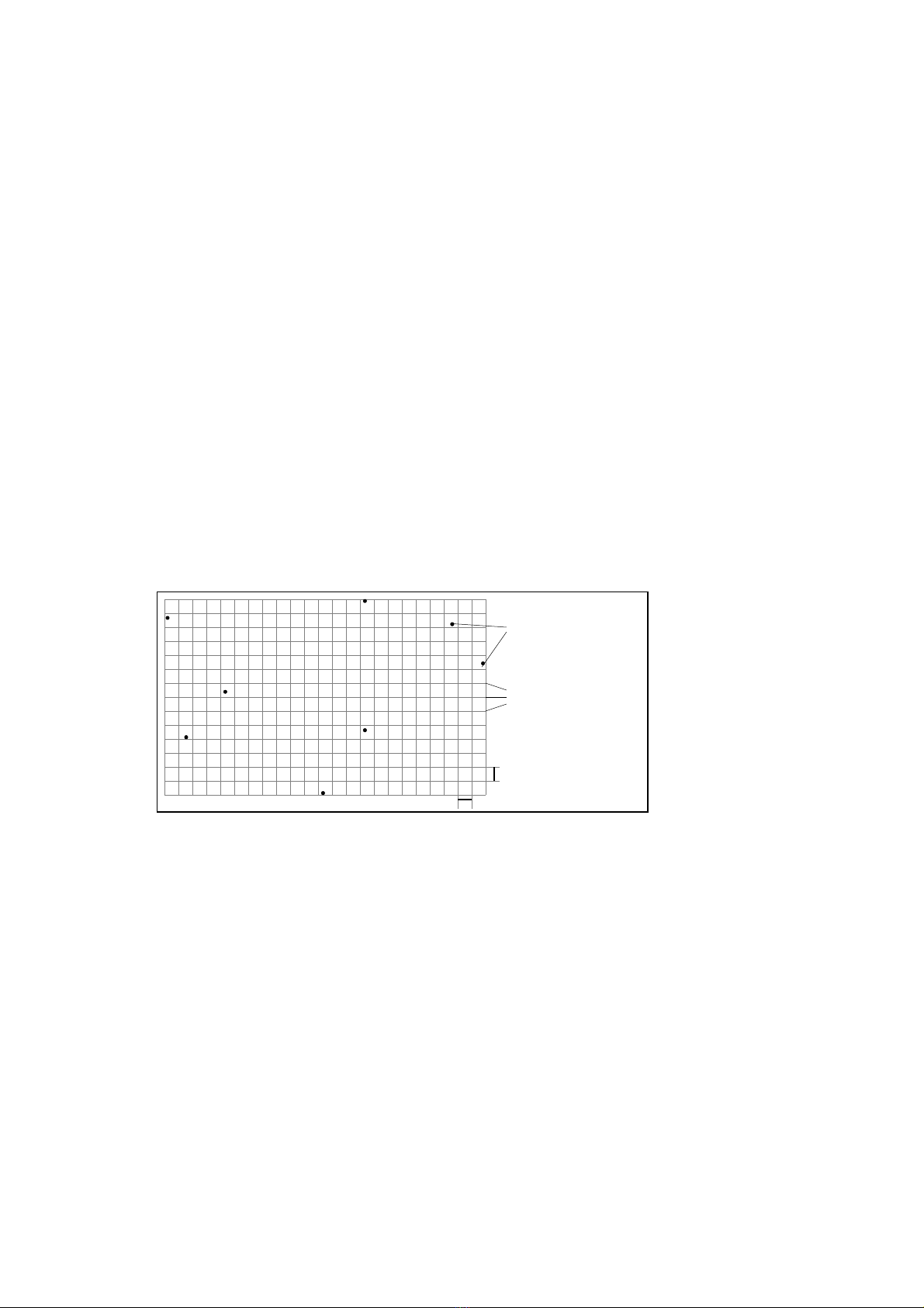
The interpolation function is determined by a matrix P of real numbers, whose elements (z-
coordinates) are assigned to nodes of a regular rectangular grid covering the domain D (see
the next figure).
Figure 2.1: Regular rectangular grid for defining the interpolation function.
The value of the interpolation function at any point
),(
00
yx
within the grid can be evalu-
ated from the equation of the bilinear polynomial
fx , y =a⋅xyb⋅xc⋅yd
, which is
defined by coordinates of corner points of the grid rectangle containing the point
),(
00
yx
.
The following notation is used in the next text:
x1 , x2
minimum and maximum of x-coordinates of points XYZ
y1 , y2
minimum and maximum of y-coordinates of points XYZ
z1 , z2
minimum and maximum of z-coordinates of points XYZ
i1 , j1
size of the grid = number of columns and rows of the matrix P
Pi,j elements of the matrix
P , i=1, ,i1 , j=1,, j1
DP auxiliary matrix with the same size as the matrix P
Z vector of z-coordinates of points XYZ
DZ auxiliary vector with the same size as the vector Z
13
step of grid in x-direction
step of grid in y-direction
points XYZ
nodes of grid

NB matrix of the nearest points - integer matrix with the same size as the matrix P con-
taining for each node of the grid the order index of the nearest point XYZ
Kmatrix of distances – integer matrix with the same size as the matrix P containing
for each node of the grid the distance to the nearest point XYZ measured in units of
grid
Kmax maximal element of the matrix K
Filter a parameter of the ABOS method used for setting resolution
RS resolution of map;
RS =max {x2−x1,y2−y1}/Filter
Dx the step of the grid in the x-direction;
Dx= x2−x1/i1−1
Dy the step of the grid in the y-direction;
Dx= y2−y1/ j1−1
Dmc the minimal Chebyshev distance between pairs of points XYZ;
Dmc=min {max {∣Xi−Xj∣,∣Yi−Yj∣} ; i≠j∧i , j=1, , n }
A→Bmeans a copy of the matrix (or vector or number) A into the matrix (or vector or
number) B
2.2 Interpolation algorithm
The algorithm of the ABOS method can be briefly described by the following scheme:
1. Filtering points XYZ, specification of the grid, computation of the matrices NB and
K, Z→DZ, 0→DP
2. Per partes constant interpolation of values DZ into the matrix P
3. Tensioning and smoothing of the matrix P
4. P+DP→P
5.
),(
iii
YXfZ
−
→DZi
6. If the maximal difference
max {DZi,i =1,, n }
does not exceed defined preci-
sion, the algorithm is finished
7. P→DP, continue from step 2 again (= start the next iteration cycle)
In the following paragraphs the particular steps of the algorithm are explained in full detail.
2.2.1 Filtering of points XYZ
If an interpolation / approximation problem has to be solved, it is necessary to take into con-
sideration the fact that there may be some points XYZ with a horizontal distance less than
the desired resolution of the resulting surface. That is why the first implemented algorithm
in the ABOS method is the filtering of points XYZ. Filtering substitutes every two points
),,(
iii
ZYX
,
),,(
jjj
ZYX
, such that
∣Xi−Xj∣ RS ∧ ∣Yi−Yj∣ RS
, (2.2.1)
by one point
),,(
kkk
ZYX
with average coordinates i.e.
2/)(
jik
XXX
+=
,
2/)(
jik
YYY
+=
and
2/)(
jik
ZZZ
+=
.
The resolution RS is computed as
max {x2−x1,y2−y1}/Filter
, where Filter is an
optional parameter of the ABOS method. It is similar to the resolution of a digital picture –
if the distance of two points with different colours is smaller than the pixel size of the digit-
al picture, only one point with “average” colour can be seen.
The formulation of the filtering principle is easy, but computer implementation represents
an efficiency problem, which is discussed in paragraph 3.4.1 Implementation of filtering in
Chapter 3.
14
2.2.2 Specification of the grid
The size of the regular rectangular grid is set according to the following points:
1. The greater side of the rectangular domain D is selected, i.e. greater number of
x21= x2−x1
and
y21= y2−y1
. Without loss of generality we can assume
that
x21
is greater.
2. The minimal grid size is computed as
i0=round x21/Dmc
, where Dmc is the
minimal Chebyshev distance between pairs of points XYZ:
Dmc=min {max {∣Xi−Xj∣,∣Yi−Yj∣} ; i≠j∧i , j=1, , n }
3. The optimal grid size is set as:
i1=max {k⋅i0 ;k=1,,5 ∧k⋅i0Filter }
4. The second size of the grid is:
j1=round y21/x21⋅i1−11
The presented procedure ensures that the difference between Dx and Dy is minimal i.e. the
regular rectangular grid is as close to a square grid as possible.
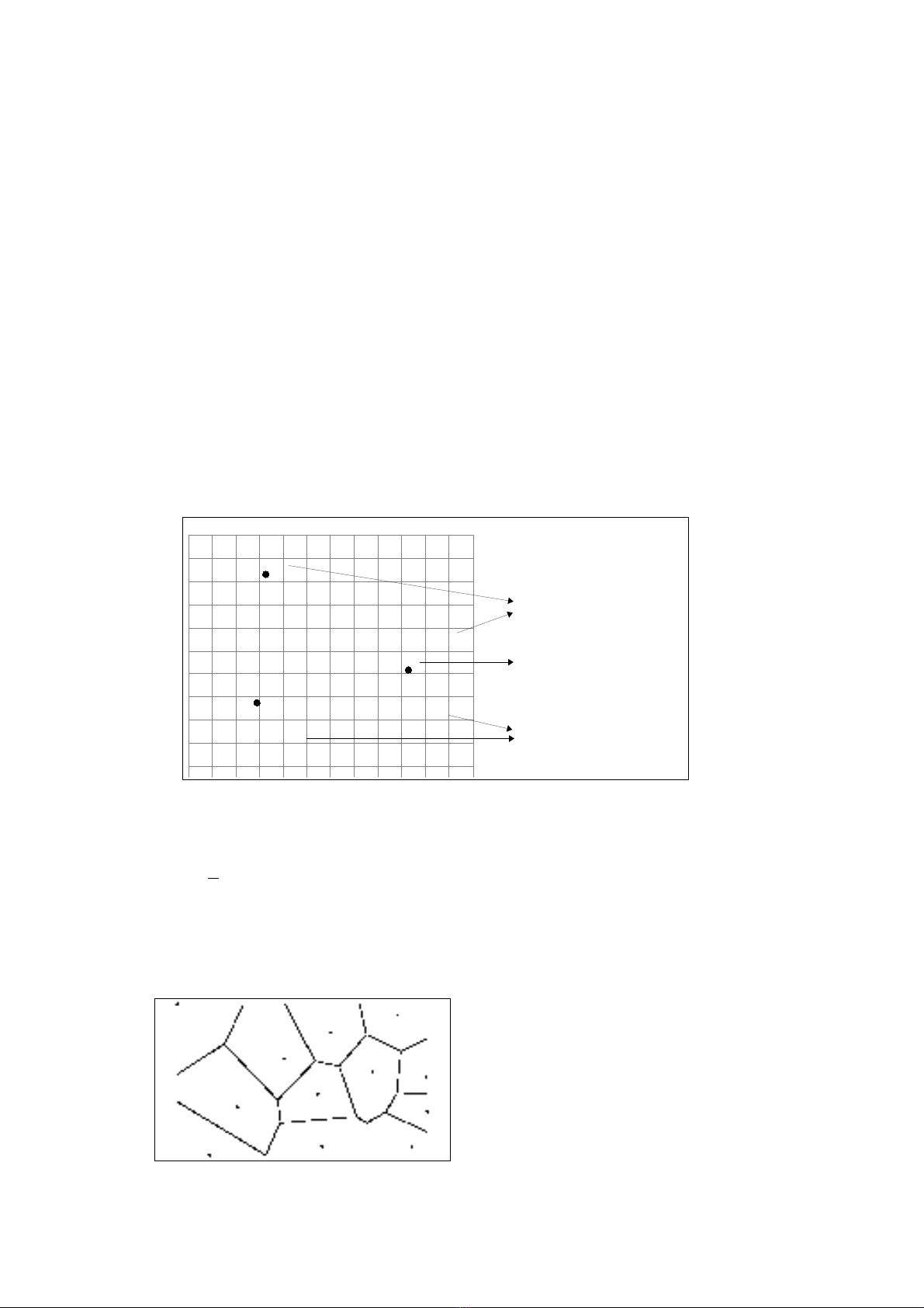
2.2.3 Computation of matrices NB and K
The matrices NB and K are computed using the algorithm based on “circulation” around the
points XYZ, as the following figure indicates:
Fig. 2.2.3a: Computation of the matrices NB and K.
All elements of the matrices NB and K are initially set to zero and the process of circulation
continues as long as there are zero values in the matrix NB. The Euclidean distance is com-
pared only if the element Ki,j corresponding to the evaluated node is not zero and
IC ∕
2≤Ki j
, where IC is the ordinal number of the current circulation. By this way,
the number of distance computations is significantly reduced.
The computation of the matrix NB defines a natural division of the domain of the interpola-
tion function into polygons (so called Voronoi or Thiessen polygons, see the following fig-
ure), inside which interpolation with constant values is performed.
Fig. 2.2.3b: Division of the domain of the interpolation function.
15
8
7
9
8 8 8 8 8
2 1 0 1 2
2 1 0 1 2
2 1 0 1 2
2 1 1 1 2
2 1 1 1 2
2 1 1 1 2
2 1 1 1 2
2 1 1 1 2
2 1 1 1 2
2 2 2 2 2
2 2 2 2 2
2 2 2 2 2
2 2 2 2 2
2 2 2 2 2
2 2 2 2 2
8 8 8 8 8
8 8 8 8 8
8 8 8 8 8
8 8 8 8 8
7 7 7 7 7
7 7 7 7 7
7 7 7 7 7
7 7 7 7 7
7 7 7 7 7
9 9 9 9 9
9 9 9 9 9
9 9 9 9 9
Number of circulations
= values of matrix K
Values of matrix NB
9 9 9 9 9
9 9 9 9 9
Ordinal index
of point XYZ
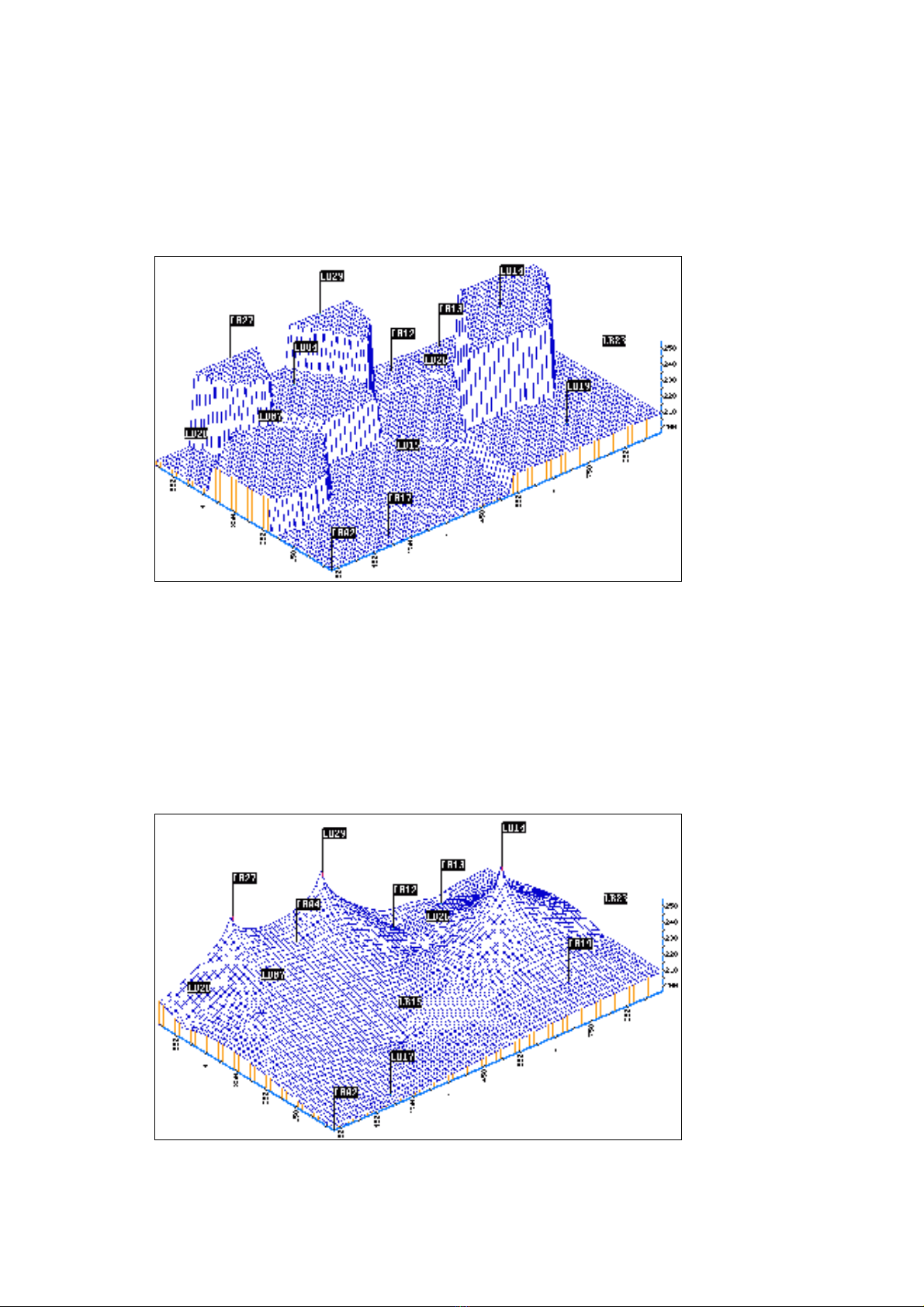
2.2.4 Per partes constant interpolation
After computing the matrix of nearest points, per partes interpolation (see figure 2.2.4) is
very simple:
)(
,, jiji
NBDZP
=
.
Fig. 2.2.4: Per partes constant interpolation.
2.2.5 Tensioning
Tensioning of the surface (see figure 2.2.5) modifies the matrix P according to the formula:
Pi , j=Pik , j Pi , jkPi−k , j Pi , j−k/4,
(2.2.5)
where
ji
Kk
,
=
,
i=1, ,i1 , j=1,, j1
Fig. 2.2.5: Tensioning of the surface.
16
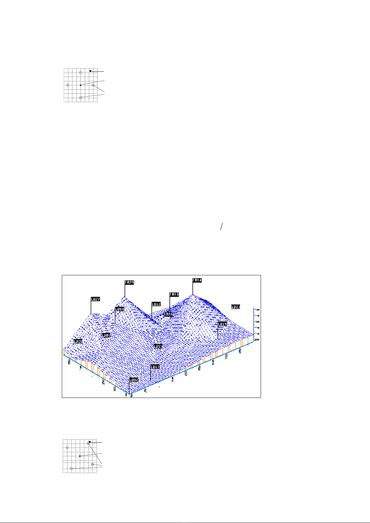
The following scheme shows the nodes (marked by grey circles) corresponding to the ele-
ments of the matrix P, which are involved in tensioning.
Tensioning is repeatedly performed in the loop with this pattern:
DO N = MAX(4,Kmax/2+2),1,-1
…
ENDDO
If k is greater than decreasing loop variable N, then k = N.
2.2.6 Linear tensioning
Linear tensioning of the surface (see figure 2.2.6) modifies the matrix P according to the
formula for weighted average:
Pi , j=Q⋅Piu , jvPi−u , j −v Pi−v , j uPiv , j−u/ 2⋅Q2
(2.2.6)
∀i=1,,i1 , j=1, , j1;Ki , j0
where
),( vu
is the vector from the node i, j to the nearest grid node of the point NBi,j and
the weight
2
,max
)(
ji
KKLQ
−⋅=
. The constant
))714,0107,0((1
maxmax
KKL
⋅−⋅=
is an
empirical constant suppressing the influence of Kmax.
In the implementation of the ABOS method there are four degrees of linear tensioning 0, 1,
2 and 3. Here presented formulas are valid for the default degree 1; their modifications for
other degrees are described in the paragraph 3.4.2 Degrees of linear tensioning.
Fig. 2.2.6: Linear tensioning of the surface.
The following scheme shows the nodes (marked by grey circles) corresponding to the ele-
ments of the matrix P, which are involved in linear tensioning.
17
grid node corresponding to the element Pi,j
nodes involved in tensioning
the nearest point XYZ
grid node corresponding to the element Pi,j
nodes involved in linear tensioning
the nearest point XYZ


![Bài tập Lập trình C++: Tổng hợp [kinh nghiệm/mới nhất/chuẩn nhất]](https://cdn.tailieu.vn/images/document/thumbnail/2025/20250826/signuptrendienthoai@gmail.com/135x160/45781756259145.jpg)