
Ann. For. Sci. 63 (2006) 687–697 687
c
INRA, EDP Sciences, 2006
DOI: 10.1051/forest:2006049 Original article
Carbon accumulation in Finland’s forests 1922–2004 – an estimate
obtained by combination of forest inventory data with modelling
of biomass, litter and soil
Jari La,b*,AleksiLc,TaruPa, Mikko Pc,ThiesEa,
Petteri Mc,RaisaM
¨
¨
¨
c
aEuropean Forest Institute, Torikatu 34, 80100 Joensuu, Finland
bFinnish Environment Institute, Research Department, Research Programme for Global Change, PO Box 140, 00251 Helsinki, Finland
cFinnish Forest Research Institute, Vantaa Research Centre, PO Box 18, 01301 Vantaa, Finland
(Received 10 October 2005; accepted 3 April 2006)
Abstract – Comparable regional scale estimates for the carbon balance of forests are needed for scientific and political purposes. We developed a
method for deriving these estimates from readily available forest inventory data by using statistical biomass models and dynamic modelling of litterand
soil. Here, we demonstrate this method and apply it to Finland’s forests between 1922 and 2004. The method was reliable, since the results obtained
were comparable to independent data. The amount of carbon stored in the forests increased by 29%, 79% of which was found in the biomass and 21%
in the litter and soil. The carbon balance varied annually, depending on the climate and level of harvesting, with each of these factors having effects
on the biomass differing from those on the litter and soil. Our results demonstrate the importance of accounting for all forest carbon pools to avoid
misleading pictures of short- and long-term forest carbon balance.
carbon inventory /forest biomass /greenhouse gas inventory /litter /soil modelling
Résumé – Accumulation de carbone dans les forêts finlandaises entre 1922 et 2004, une estimation obtenue en combinant les données de
l’inventaire forestier avec une modélisation de la biomasse de la litière et du sol. Une estimation comparable à l’échelle régionale du bilan de
carbone des forêts était nécessaire pour des objectifs scientifiques et politiques. Nous avons développé une méthode pour déduire ces estimations de
données facilement disponibles de l’inventaire forestier en utilisant des modèles statistique de la biomasse et une modélisation dynamique de la litière
et du sol. Ici nous présentons cette méthode et l’appliquons aux forêts de Finlande entre 1922 et 2004. La méthode a été fiable, puisque les résultats
obtenus ont été comparables à des données indépendantes. La quantité de carbone accumulée dans les forêts s’est accrue de 29 %,79 % de ce qui a été
trouvé dans la biomasse et 21 % dans la litière et le sol. Le bilan de carbone varie annuellement, selon le climat et l’importance de la récolte, chacun
de ces facteurs ayant des effets sur la biomasse différents de ceux qui agissent sur la litière et sur le sol. Nos résultats démontrent l’importance de
comptabiliser tous les réservoirs de carbone en forêt pour éviter des images trompeuses du bilan de carbone des forêts à court et moyen terme.
inventaire du carbone /biomasse forestière /inventaire des gaz à effet de serre /litière /sol
1. INTRODUCTION
Forests may act both as important sinks and as sources of
atmospheric carbon dioxide (CO2) [18]. Therefore, to under-
stand the development of the atmospheric CO2concentration
and, consequently, changes in the world’s climate, it is neces-
sary to know the carbon balance of forests and the processes
and factors controlling it.
This importance of forests has been recognized in the
United Nations Framework Convention on Climate Change
(UNFCCC) [71], which enjoins countries to include changes
in forest carbon stocks in their annual greenhouse gas (GHG)
inventories. In addition, the Kyoto Protocol states that some of
these changes will be accounted for in the GHG emissions of
* Corresponding author: jari.liski@ymparisto.fi
countries during the first commitment period of limiting these
emissions between 2008 and 2012 [72].
Acknowledging that it is the entire forest carbon balance
that is crucially linked to the atmosphere, not only the balance
of some parts of it, the 7th Conference of Parties (COP) to
the UNFCCC agreed that countries must account for all forest
carbon pools in their annual GHG inventories and under the
Kyoto Protocol [19]. The COP named these pools as above-
and belowground biomass, deadwood, litter and soil organic
carbon. Thus, in addition to the scientific need, there is also
an urgent political need for reliable accounting of all forest
carbon pools.
In many industrialized countries, the national estimates for
the carbon balance of tree biomass are calculated based on data
from national forest inventories (NFI) [41]. The NFIs in gen-
eral provide statistically sound estimates of forest resources,
and these estimates are characterized by a small sampling
Article published by EDP Sciences and available at http://www.edpsciences.org/forest or http://dx.doi.org/10.1051/forest:2006049

688 J. Liski et al.
error because the measurements are taken at thousands of for-
est sites [28, 70]. In addition, it is a fairly straightforward
matter to estimate the carbon balance of tree biomass based
on the inventory data on stem volume, using conversion fac-
tors available for many tree species and geographical regions
[21,30,32,62,65,74,75,78].
In contrast, readily available methods for estimating the
carbon balances of the nonliving organic matter pools are
still lacking. Measuring the carbon balances of litter and soil
organic matter is particularly difficult because the expected
changes [37, 60] are one or two orders of magnitude smaller
than the spatial variability inside forest sites [33]. For this
reason, various modelling approaches were applied to obtain
these estimates [14,25,37,58]. The diversity of these methods
makes, however, comparison of the results difficult [9].
We developed a method for estimating the total carbon bal-
ance of forests based on NFI data. Here, we demonstrate this
method and test its applicability and reliability by applying
it to Finland’s forests between the 1920s and 2000s. In addi-
tion, we explore the variability in the carbon balance of these
forests and factors that caused it. Based on these results, we
analyse the importance of natural and human-induced factors
for the carbon balance of these managed forests and discuss
the rationality for the reporting requirements of the UNFCCC.
2. MATERIAL AND METHODS
2.1. Calculation method
The calculation method is based on forest inventory measurements
of forest area and stem volume. The pools and fluxes of carbon in
forests are estimated from the inventory data with the aid of mod-
elling. The biomasses of the various components of trees are calcu-
lated using biomass expansion factors, and the biomass of ground
vegetation is obtained using other statistical models. The litter pro-
duction of vegetation is calculated by multiplying these biomass es-
timates by compartment-specific turnover rates. The carbon pools of
litter (including deadwood) and soil organic matter as well as the cy-
cling of carbon in these pools are simulated using a dynamic model.
The basic concepts of this calculation method were presented earlier
[37], but here we demonstrate a more advanced version of the method
consisting of new models shown to be appropriate for regional and
national scale inventories.
2.2. Application to Finland’s forests
We applied this calculation method to Finland’s forests from 1922
to 2004. The calculations were conducted for the main tree species,
i.e. Scots pine (Pinus sylvestris L.), Norway spruce (Picea abies (L.)
Karsten) and broadleaved trees (mainly silver birch Betula pendula
Roth and downy birch B. pubescens Ehrh.), and separately for the
southern and northern parts of the country. The pine forests covered
49–66% of the total forested area during the period studied, the spruce
forests 23–36% and the broadleaved forests 7–15%. Our results for
trees cover all forest land including both upland forests and peat-
lands, whereas our results for soil, litter and ground vegetation are
for upland forests only because we had no appropriate models for
these components on peatlands. Moreover, in Finland’s reports for
Figure 1. Growing stock, gross annual increment, drain (fellings plus
natural losses) and area of Finland’s forests between 1922 and 2004.
the UNFCCC, GHG accounting of peatland soils is based on mea-
surements of GHG fluxes for different ecosystem types and corre-
sponding areal estimates, not on estimates of changes in the carbon
stock of these soils [19]. The upland forests represented 74–79% of
the total forested area during the period studied.
2.2.1. Forest inventory data
The NFI has been conducted in Finland nine times so far (Fig. 1),
each time requiring three to nine years to inventory the entire coun-
try. The first NFI in 1921–1924 was a line transect survey, with the
length of the surveyed line totalling more than 13 000 km and the
distance between the survey lines being 26 km [17], whereas the last
NFI applied systematic cluster sampling and obtained measurements
at about 70 000 sites [67].
The volume of the growing stock of trees (GS,m
3)wasgivenby
age-class in the two latest NFIs, while the earlier NFIs provided it in
total and only the forested areas by age-class. To estimate the GS dis-
tribution between the age-classes in these earlier NFIs, we assumed
that the shape of the distribution of the mean volume (m3/ha) be-
tween the age-classes had remained the same as in the eighth NFI
and, consequently, divided the total volume into age-classes using
the age-class-specific data on forested areas.
To obtain the annual values for the GS volume, we first estimated
annual gross increment (GAI,m
3). GAI at year Tbetween two con-
secutive NFIs, Nand N+1, having the volume weighted midyears TN
and TN+1, was calculated by scaling the average growth during the
period with growth indices, gi,T
GAIi(T)=gi,T
GS i,TN+1−GS i,TN+diD(TN,TN+1)
TN+1−TN
·
In this equation, iis specific for tree species and age-class and
D(TN,TN+1) (m3) is the sum of drain between the midyears of the in-
ventories; Dincludes commercial fellings, domestic wood use and
natural mortality (mortality of trees from causes other than cutting by
man). The drain estimates were reported by Forest Statistics Informa-
tion Service at the Finnish Forest Research Institute; information on
the commercial fellings was based on reports by the major industrial
wood users [45]. Variable direpresents division of drain between tree
species and age-classes i. The fellings were allocated to age-classes
by estimating the age distribution of cuttings and thinning at the per-
manent sample plots of the NFI. The gireflect the climate-induced

Carbon sink of Finland’s forests 689
Tab le I. Biomass turnover rates (year−1) used to estimate the litter production of trees and ground vegetation.
Trees
Spruce forests Pine forests Broadleaved forests
S1N2SNSN
Foliage 0.1030.0530.2240.1040.785
Branches and roots 0.01253f(t)60.01357
Stump bark 0.080.003090.000110
Reproductive origins and stem bark 0.002780.005290.002910
Fine roots 0.81111 0.86812 1.013
Ground vegetation
Bryophytes 0.3314
Lichens 0.115
Dwarf shrubs, aboveground 0.2516
Herbs and grasses, aboveground 1.017
Dwarf shrubs, belowground 0.3318
Herbs and grasses, belowground 0.3316
1Southern Finland. 2Northern Finland. 3[51]. 4[50]. 5Leaves of broadleaved trees became 22% lighter during yellowing process in autumn [77]. 6As
a function of age [31]. 7Estimated from the repeatedly measured permanent sample plots of the Finnish National Forest Inventory. 8Derived from the
results of Viro [77]. 9Derived from the results of Viro [77] and Mälkönen [54]. 10 Derived from the results of Viro [77] and Mälkönen [55]. 11 [42].
12 [26]. 13 We assumed that broadleaved trees replace all their fine roots each year. 14 Rough estimation that the litter fall equals the annual biomass
production [12, 23, 57, 64]. 15 Rough estimation that the litter fall equals the annual biomass production [24, 39]. 16 Rough estimation that the litter fall
equals the annual biomass production [12, 49, 54]. 17 Aboveground parts of herbs and grasses change completely into litter at the end of the growing
season. 18 Rough estimation that the life expectancy for roots is about 2–3 years [13].
annual variability in tree growth with no trend like changes, and was
based on field measurements of several hundreds of trees as part of
the NFI [16, 46, 66]. The last givalues were available for year 2000
for pine in southern Finland and 1993 for all the other tree species and
regions. For this reason, only limited variation occurred in our growth
estimates after 1993 and none after 2000. For all deciduous forests,
we applied the mean gvalue of pine and spruce because there were
no specific values for the broadleaved species. Finally, we calculated
the annual values for the GS volume between the inventory midyears
by adding GAI to and subtracting Dfrom the previous year’s estimate
of GS.
2.2.2. Biomass
The estimates for the GS volume were converted to biomass us-
ing biomass expansion factors specific for tree species, stand age and
biomass component (foliage, branches, stem wood, bark, stump and
transportation roots) [30].
Suitable factors were available for neither the fine roots of
any forests nor for the stumps, transportation roots or foliage of
broadleaved forests. To estimate the biomasses of these components,
we assumed that the fine root biomass of conifers was proportional to
foliage biomass and estimated these proportions from studies of both
foliage and fine root biomasses [5, 15, 76]. For pine forests, this pro-
portion was 50% and for spruce forests 30%, while for broadleaved
forests, we assumed that the ratio between fine root and stem biomass
was the same as in pine forests of the same age. The compounded
biomass of the stumps and transportation roots was assumed to be
53% of the stem biomass in broadleaved forests [27] and we divided
this biomass equally between these components. We assumed that
the leaf biomass of broadleaved forests was proportional to branch
biomass and that this proportion decreased from 80% to 20% with
increasing stand age of from 10 to 150 years.
The biomass of ground vegetation was estimated using regression
models that give the biomass of various species groups based on stand
age and dominant tree species [52, 60]. There were separate models
for pine and spruce forests; for broadleaved forests, we applied the
latter. All biomass estimates were converted to carbon by multiplying
by 0.5 [19].
2.2.3. Litter production
The calculation method distinguishes three carbon fluxes from
forest biomass to litter and soil: (1) the litter production of living
vegetation resulting from biomass turnover, (2) the mortality of tree
individuals due to natural causes and (3) the harvest residues. We cal-
culated the first of these fluxes by multiplying the biomass estimates
by biomass turnover rates (Tab. I). The second flux was taken to be
equal to the biomass of dying trees, and this biomass was added to the
litter and soil pools as soon as the trees were dead. The third flux was
assumed to be equal to the biomass of trees felled, excluding 91% of
the stem biomass that was removed from the forests.
2.2.4. Litter and soil
The carbon pools of litter and soil organic matter, the annual
changes in these pools and heterotrophic respiration (Rh) resulting
from decomposition were calculated using the Yasso dynamic soil
carbon model [36]. This model simulates cycling of carbon in upland
forest soils to a depth of 1 m in mineral soil.
Yasso consists of five decomposition compartments and two
woody litter compartments (Fig. 2). The dynamics of carbon in these
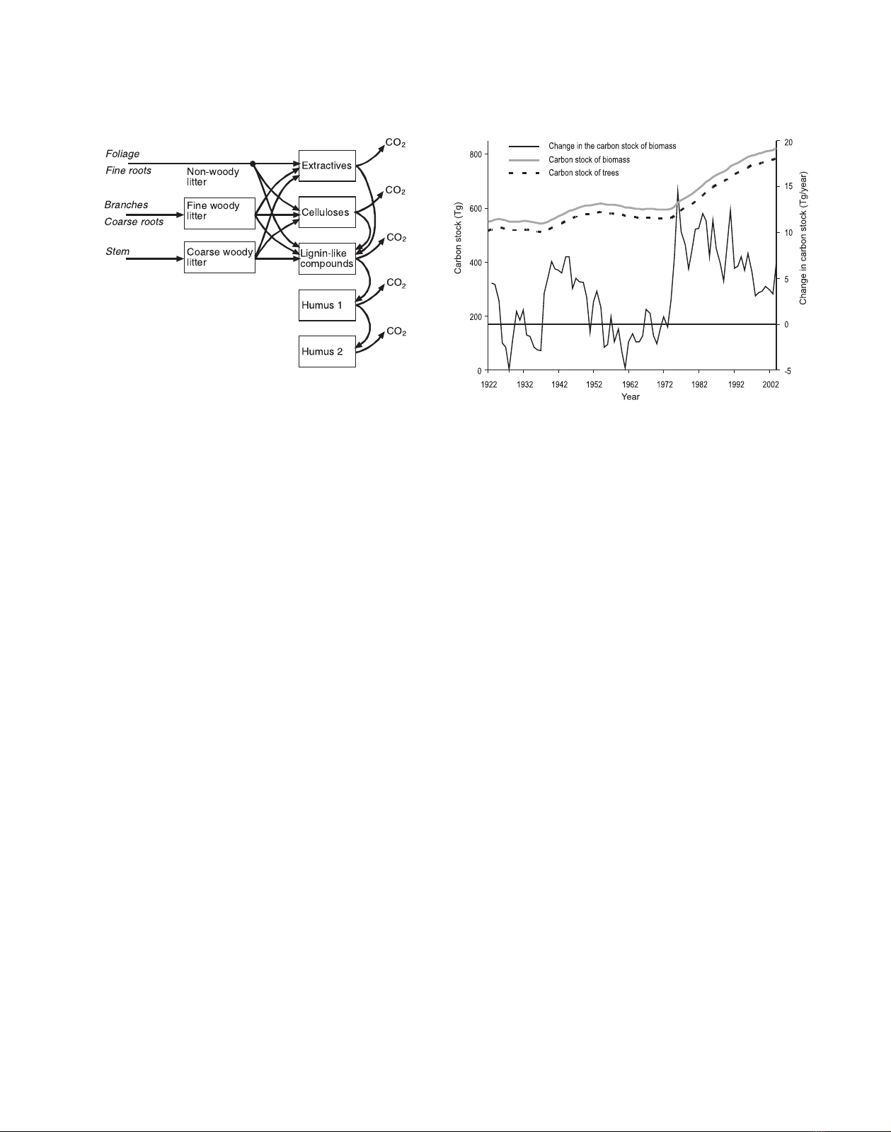
690 J. Liski et al.
Figure 2. Flow chart of the Yasso litter and soil carbon model. The
boxes represent carbon compartments and the arrows carbon fluxes.
Reprinted from [36], with permission from Elsevier.
compartments is controlled by the physical and chemical character-
istics of litter and climate. The chemical characteristics of litter are
accounted for by dividing litter between three decomposition com-
partments having different decomposition rates. One of these com-
partments is for the most easily decomposable compounds, while
the others are for cellulose and lignin; division is done according to
the actual concentrations of these compounds in the litter. The re-
maining two decomposition compartments are for humus formed in
the decomposition process. The physical characteristics of litter are
accounted for by dividing woody litter between the compartments
of fine (branches and transportation roots) and coarse woody litter
(stem and stump) and releasing it for actual decomposition at higher
rates from the compartment of fine woody litter. The climatic con-
trols of decomposition in the Yasso model are temperature and sum-
mer drought. In the present study, we excluded the effects of summer
drought because temperature alone explains more than 85% of the cli-
matic effects on decomposition on an annual basis in Finland [35,47].
We calculated the values for the effective temperature sum based on
CRU TS 1.2 data set (Mitchell et al., unpublished manuscript).
The soil and litter carbon pools at the beginning of the study pe-
riod were calculated by assuming a steady state with mean litter in-
put between 1922 and 1936 and mean temperature between 1901 and
1930. Starting from this steady state in 1922, the model was run using
annually varying values of litter input and temperature.
In addition to litter production of forest vegetation and removals of
carbon as a result of Rh, the soil and litter carbon balance in Finland’s
forests was affected by changes in land use. Conversion of other types
of land to forest introduced carbon to the soil and litter of the forests,
whereas conversion of forest to some other land type removed car-
bon. We did not know the carbon contents of afforested or deforested
land and therefore assumed that all this land had the same carbon
content (6.1 kg/m2), which was the mean value for soil and litter at
the beginning of our calculations. To estimate the amounts of carbon
transferred between forests and other land uses, we multiplied the an-
nual net changes in forested area by this figure. To follow the effects
of this carbon on the carbon balance of forest soils, we divided it
into the compartments of the Yasso model according to the division
of the steady-state stock in 1922 and used this model to simulate its
dynamics in the forests.
Figure 3. Carbon stock of biomass (trees plus ground vegetation),
carbon stock of trees alone and annual changes in the carbon stock of
biomass in Finland’s forests between 1922 and 2004.
2.3. Ecological concepts
To enable comparison of our results with those of other ecological
studies, we calculated values for the ecological concepts of the forest
carbon cycle (e.g. [18]) from our inventory-based estimates. In the
equations that follow, the terms used in forest inventories are marked
between quotes and are represented as converted to carbon in whole-
tree biomass; the international definitions of these terms are given in
[70].
The estimate for net primary production (NPP) was calculated by
summing the change in the growing stock of trees ∆GS, change in
the biomass of ground vegetation ∆B, litter production of trees and
understorey L, natural losses (mortality) of trees Mand fellings (har-
vesting) of trees by humans F
NPP =“∆GS ”+∆B+L+“M”+“F”.
The estimate for net ecosystem production (NEP) was obtained by
subtracting Rh from NPP which was simulated using the Yasso soil
model
NEP =NPP −Rh.
The net biome production (NBP) was calculated by subtracting from
NEP removals (RE) that represented felled roundwood removed from
the forests
NBP =NEP −“RE”.
3. RESULTS
3.1. Carbon balance of biomass
The biomass carbon stock increased by 50%, from 550 to
823 Tg, in Finland’s forests between 1922 and 2004 (Fig. 3).
This increase, equal to an average of 3.3 Tg/year, was due
to both a higher mean amount of carbon per forested area in
forests remaining as forests and an expanded forested area (see
Fig. 1). Carbon accumulated mainly in the biomass of trees,
Carbon sink of Finland’s forests 691
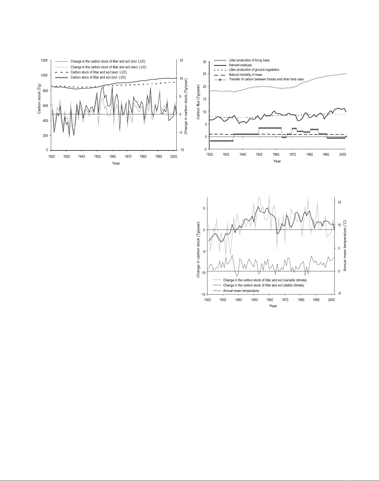
Figure 4. Carbon stock of litter and soil and its annual changes
in Finland’s forests between 1922 and 2004. The black lines show
these variables when the transfers of carbon in litter and soil between
forests and other land uses were accounted for (incl. LUC) and the
grey lines show these variables when these transfers were ignored
(excl. LUC).
whereas our estimate for the biomass of ground vegetation re-
mained relatively stable (Fig. 3). The mean biomass carbon
stock was 3.1 kg/m2in 1922 and 4.0 kg/m2in 2004.
Despite this trend towards increase, the annual changes in
the biomass carbon stock were highly variable (Fig. 3). The
biomass gained 14.5 Tg of carbon in an extreme year in the
1970s and lost 5.0 Tg in another year in the 1920s.
This high annual variability was caused by changes in tree
growth and harvesting. In the 1920s, 1930s, 1950s and 1960s
harvesting exceeded tree growth, thus decreasing the carbon
stock of trees, whereas in the 1940s during and after World
War II large amounts of carbon accumulated in tree biomass
since the level of harvesting was low (Figs. 1 and 3). The tree
carbon stock also rapidly increased since the 1970s despite the
greater harvests as a result of increased tree growth.
3.2. Carbon balance of litter and soil
The carbon stock of litter and soil increased by 13%, from
848 to 959 Tg, during the 82-year period studied, when the
transfers of carbon between the forests and other land uses
were accounted for (Fig. 4). When these transfers were ig-
nored, the carbon stock increased by 7%, from 848 to 905 Tg.
In the former case, the mean accumulation rate of carbon was
1.4 Tg/year and, in the latter case, 0.7 Tg/year. The mean car-
bon content of the soils was 6.1 kg/m2in 1922 and increased
to 6.3 kg/m2in 2004 when the transfers of carbon between the
forests and other land uses were accounted for.
The interannual changes in the litter and soil carbon stock
also varied widely (Fig. 4). Our highest estimates for the an-
nual increases and decreases were 7.5 and 5.8 Tg/year, respec-
tively, when the transfers of litter and soil carbon between the
Figure 5. Input of carbon to the carbon stock of litter and soil by
origin, and the transfers of carbon in litter and soil between forests
and other land uses in Finland’s forests between 1922 and 2004.
Figure 6. Annual changes in the carbon stock of litter and soil in Fin-
land’s forests between 1922 and 2004 when the transfers of carbon in
litter and soil between forests and other land uses were accounted for
(incl. LUC), simulated using the actual variable climatic conditions
or stable average climate. The annual mean temperature of Finland is
also shown.
forests and other land uses were accounted for and 5.3 and
2.9 Tg/year when these transfers were ignored.
There were three causes for this increase and the annual
variation in the litter and soil carbon stock: (1) transfers of
litter and soil carbon between the forests and other land uses,
(2) litter input to the soils and (3) temperatures that affected the
rates of decomposition. Among these factors, litter input from
living trees and the transfers of soil carbon from other land
uses appeared as the major causes for the increase (Fig. 5). The
annual changes, on the other hand, were caused mainly by the
variability in temperature (Fig. 6) and harvest residues (Fig. 5).
Among these two factors, the harvest residues were slightly
more important because more than half of the variability still


%20--%3e%3cdefs%3e%3cstyle%3e%20.st0%20{%20fill:%20%23fff;%20}%20.st1%20{%20fill:%20%237800fa;%20}%20%3c/style%3e%3c/defs%3e%3cpath%20class='st1'%20d='M117.78,12.18H43.11c2.9,3.47,4.65,7.94,4.65,12.82,0,5.6-2.3,10.66-6.01,14.29h76.02l7.22-13.56-7.22-13.56Z'/%3e%3cg%3e%3cpath%20class='st0'%20d='M53.58,26.17h-.59v-1.46h.59v-4.96h2.83c1.78,0,2.67.94,2.67,2.82v5.76c0,1.87-.89,2.81-2.67,2.81h-2.83v-4.96ZM55.36,21.37v3.34h1.1v1.46h-1.1v3.34h1.01c.61,0,.91-.37.91-1.1v-5.93c0-.74-.3-1.1-.91-1.1h-1.01Z'/%3e%3cpath%20class='st0'%20d='M65.99,31.14h-1.8l-.31-2.07h-2.19l-.31,2.07h-1.64l1.82-11.39h2.62l1.82,11.39ZM65.28,18.04c-.25.46-.51.77-.75.94-.21.15-.47.22-.79.22-.26,0-.57-.07-.92-.22l-.38-.15c-.14-.05-.26-.07-.37-.07-.3,0-.53.18-.71.54l-.91-.68c.25-.46.51-.77.75-.94.21-.14.48-.21.79-.21.26,0,.57.07.92.21l.38.15c.14.05.26.07.37.07.3,0,.53-.18.71-.54l.91.68ZM61.91,27.52h1.73l-.87-5.76-.87,5.76Z'/%3e%3cpath%20class='st0'%20d='M74.53,26.89v1.52c0,1.91-.89,2.86-2.67,2.86s-2.67-.95-2.67-2.86v-5.93c0-1.91.89-2.86,2.67-2.86s2.67.95,2.67,2.86v1.11h-1.69v-1.22c0-.75-.31-1.12-.93-1.12s-.93.37-.93,1.12v6.15c0,.74.31,1.11.93,1.11s.93-.37.93-1.11v-1.63h1.69Z'/%3e%3cpath%20class='st0'%20d='M81.4,31.14h-1.8l-.31-2.07h-2.19l-.31,2.07h-1.64l1.82-11.39h2.62l1.82,11.39ZM75.9,19.2l1.52-1.91h1.71l1.51,1.91h-1.61l-.76-.95-.75.95h-1.61ZM77.32,27.52h1.73l-.87-5.76-.87,5.76ZM83.1,15.99l-1.76,1.91h-1.26l1.17-1.91h1.86Z'/%3e%3cpath%20class='st0'%20d='M84.86,19.75c1.78,0,2.67.94,2.67,2.82v1.48c0,1.87-.89,2.81-2.67,2.81h-.85v4.28h-1.79v-11.39h2.64ZM84.01,21.37v3.86h.85c.58,0,.87-.36.87-1.08v-1.71c0-.71-.29-1.07-.87-1.07h-.85Z'/%3e%3cpath%20class='st0'%20d='M93.51,19.75c1.78,0,2.67.94,2.67,2.82v1.48c0,1.87-.89,2.81-2.67,2.81h-.85v4.28h-1.79v-11.39h2.64ZM92.66,21.37v3.86h.85c.58,0,.87-.36.87-1.08v-1.71c0-.71-.29-1.07-.87-1.07h-.85Z'/%3e%3cpath%20class='st0'%20d='M98.8,31.14h-1.79v-11.39h1.79v4.88h2.03v-4.88h1.83v11.39h-1.83v-4.88h-2.03v4.88Z'/%3e%3cpath%20class='st0'%20d='M105.36,24.55h2.46v1.62h-2.46v3.34h3.09v1.63h-4.88v-11.39h4.88v1.63h-3.09v3.18ZM108.17,17.29l-1.76,1.91h-1.26l1.17-1.91h1.86Z'/%3e%3cpath%20class='st0'%20d='M112.2,19.75c1.78,0,2.67.94,2.67,2.82v1.48c0,1.87-.89,2.81-2.67,2.81h-.85v4.28h-1.79v-11.39h2.64ZM111.35,21.37v3.86h.85c.58,0,.87-.36.87-1.08v-1.71c0-.71-.29-1.07-.87-1.07h-.85Z'/%3e%3c/g%3e%3ccircle%20class='st1'%20cx='25'%20cy='25'%20r='20'/%3e%3cpath%20class='st0'%20d='M32.78,19.27c2.92,0,4.43,2.55,5.28,5.33l.71,2.17c.14.38-.33.75-.71.75h-5.61c.19-.33.24-.71.09-1.08l-.75-2.45c-.43-1.32-.99-2.64-1.79-3.77.75-.57,1.65-.94,2.78-.94h0ZM25,18.38c3.25,0,4.9,2.78,5.89,5.89l.76,2.45c.14.42-.33.8-.8.8h-11.69c-.42,0-.94-.38-.8-.8l.75-2.45c.99-3.11,2.64-5.89,5.89-5.89h0ZM25,11.35c1.74,0,3.11,1.37,3.11,3.11s-1.37,3.11-3.11,3.11-3.11-1.41-3.11-3.11,1.41-3.11,3.11-3.11h0ZM17.27,19.27c1.08,0,1.98.38,2.73.94-.8,1.13-1.37,2.45-1.74,3.77l-.8,2.45c-.14.38-.05.75.09,1.08h-5.56c-.42,0-.9-.38-.75-.75l.71-2.17c.9-2.78,2.41-5.33,5.33-5.33h0ZM17.27,12.91c1.51,0,2.78,1.27,2.78,2.83s-1.27,2.83-2.78,2.83-2.83-1.27-2.83-2.83,1.27-2.83,2.83-2.83h0ZM32.78,12.91c1.56,0,2.78,1.27,2.78,2.83s-1.23,2.83-2.78,2.83-2.83-1.27-2.83-2.83,1.27-2.83,2.83-2.83h0ZM27.07,28.56v.09c0,.57-.24,1.08-.61,1.46h0v.05c-.38.33-.9.57-1.46.57s-1.08-.24-1.46-.61h0c-.38-.38-.61-.9-.61-1.46v-.09h1.41v.09c0,.19.05.38.19.47v.05c.09.09.28.19.47.19s.38-.09.47-.19v-.05c.14-.09.24-.28.24-.47t-.05-.09h1.41ZM30.99,28.56v.09c0,1.65-.66,3.16-1.74,4.24-1.08,1.08-2.59,1.79-4.24,1.79s-3.16-.71-4.24-1.79l-.05-.05c-1.04-1.08-1.7-2.55-1.7-4.2v-.09h1.41v.09c0,1.27.47,2.4,1.27,3.25h.05c.85.85,1.98,1.37,3.25,1.37s2.4-.52,3.25-1.37c.85-.8,1.37-1.98,1.37-3.25v-.09h1.37ZM34.99,28.56v.09c0,2.78-1.13,5.28-2.92,7.07-1.79,1.79-4.29,2.92-7.07,2.92s-5.23-1.13-7.07-2.92c-1.79-1.79-2.92-4.29-2.92-7.07v-.09h1.41v.09c0,2.4.94,4.53,2.5,6.08,1.56,1.56,3.72,2.5,6.08,2.5s4.52-.94,6.08-2.5c1.56-1.56,2.5-3.68,2.5-6.08v-.09h1.41Z'/%3e%3c/svg%3e)