
Hindawi Publishing Corporation
EURASIP Journal on Advances in Signal Processing
Volume 2009, Article ID 784379, 7pages
doi:10.1155/2009/784379
Research Article
Removing the Influence of Shimmer in the Calculation
of Harmonics-To-Noise Ratios Using Ensemble-Averages
in Voice Signals
Carlos Ferrer, Eduardo Gonz´
alez, Mar´
ıa E. Hern´
andez-D´
ıaz,
Diana Torres, and Anesto del Toro
Center for Studies on Electronics and Information Technologies, Central University of Las Villas, C. Camajuan´
ı,
km 5.5, Santa Clara, CP 54830, Cuba
Correspondence should be addressed to Carlos Ferrer, cferrer@uclv.edu.cu
Received 1 November 2008; Revised 10 March 2009; Accepted 13 April 2009
Recommended by Juan I. Godino-Llorente
Harmonics-to-noise ratios (HNRs) are affected by general aperiodicity in voiced speech signals. To specifically reflect a signal-to-
additive-noise ratio, the measurement should be insensitive to other periodicity perturbations, like jitter, shimmer, and waveform
variability. The ensemble averaging technique is a time-domain method which has been gradually refined in terms of its sensitivity
to jitter and waveform variability and required number of pulses. In this paper, shimmer is introduced in the model of the ensemble
average, and a formula is derived which allows the reduction of shimmer effects in HNR calculation. The validity of the technique
is evaluated using synthetically shimmered signals, and the prerequisites (glottal pulse positions and amplitudes) are obtained by
means of fully automated methods. The results demonstrate the feasibility and usefulness of the correction.
Copyright © 2009 Carlos Ferrer et al. This is an open access article distributed under the Creative Commons Attribution License,
which permits unrestricted use, distribution, and reproduction in any medium, provided the original work is properly cited.
1. Introduction
When the source-filter model of speech production [1]
is assumed in Type 1 [2] signals (no apparent bifurca-
tions/chaos), the sources of periodicity perturbations in
voiced speech signals can be divided in four classes [3]:
(a) pulse frequency perturbations, also known as jitter, (b)
pulse amplitude perturbations, also known as shimmer, (c)
additive noise, and (d) waveform variations, caused either by
changes in the excitation (source) or in the vocal tract (filter)
transfer function. Vocal quality measurements have focused
mainly in the first three classes (see [4] for a comprehensive
survey of methods reported in the previous century). The
findings of significant interrelations among measures of
jitter, shimmer, and additive noise [5] raised the question on
“whether it is important to be able to assign a given acoustic
measurement to a specific type of aperiodicity” (page 457).
This ability of a measurement to gauge a particular signal
attribute, being insensitive to other factors, has been a
persistent interest in vocal quality research.
Harmonics-to-Noise-Ratios (HNRs) have been proposed
as measures of the amount of additive noise in the acoustic
waveform. However, an HNR measure insensitive to all
the other sources of perturbation is, if feasible, still to be
found. Methods in both time and frequency (or trans-
formed) domain do always have intrinsic flaws. Schoentgen
[6] described analytically the effects of the different per-
turbations in the Fourier spectra of source and radiated
waveforms. According to the derivations from his models,
it is not possible to perform separate measurements of
each type of perturbation by using spectral-based methods.
Time domain methods have been criticized [7,8]for
depending on the correct determination of the individ-
ual pulse boundaries, among many other method-specific
factors.
Yumoto et al. introduced a time-domain method for
determining HNR [9], where the energy of the harmonic
(repetitive) component is equal to the variance of a pulse
“template” obtained as the ensemble average of the individ-
ual pulses. The energy of the noise component is calculated

2 EURASIP Journal on Advances in Signal Processing
as the variance of the differences between the ensemble and
the template (see (4)inSection 2).
The original ensemble-averaging technique has been
criticized [10,11] for its slow convergence with N, the
number of averaged pulses. The requirement of large N
facilitates the inclusion of slow waveform changes in the
ensemble, which are incorrectly treated as noise by the
method. The sensitivity of the method to jitter and shimmer
has also been reported [5], and many approaches attempting
to overcome these limitations have been proposed.
In [12] the need of averaging a large number of pulses is
suppressed, by determining an expression which corrects the
ensemble-average HNR.
Qi et al. used Dynamic Time Warping (DTW) [13]
and later Zero Phase Transforms (ZPTs) [14] of individual
pulses prior to averaging to reduce waveform variability (and
jitter) influences in the template. For the same purpose the
ensemble averaging technique was applied to the spectral
representations of individual glottal source pulses in [3],
where a pitch synchronous method allowed to account for
jitter and shimmer in the glottal waveforms. However, the
assumptions are valid only on glottal source signals; hence
results are not applicable to vocal tract filtered signals.
Functional Data Analysis (FDA) has also been used to
perform the optimal time alignment of pulses prior to
averaging [15].
Shimmer corrections to ensemble averages HNRs have
received lesser attention than pulse duration (jitter) cor-
rections, in spite of being a prerequisite for some of the
mentioned jitter correction methods. DTW and FDA, for
instance, depart from considering equal amplitude pulses
to determine the required expansion/compression of the
waveform duration. Besides, shimmer always increases the
variability of the ensemble with respect to the template in the
reported methods. A normalization of each individual pulse
by its RMS value was proposed in [7] to reduce shimmer
effects on HNR and was first used on a method that also
accounted for jitter and offset effects in [16]. This pulse
amplitude (shimmer) normalization can help in the time
warping of the pulses and actually reduces the variance of the
template in Yumoto’s HNR formula. However, it still yields
only an approximate value of HNR.
In this paper, an analysis on the original ensemble average
HNR formula in the presence of shimmer is performed,
which results in a general form of Ferrer’s correcting formula
[12] and allows the suppression of the effect of shimmer in
HNR.
2. Ensemble-Averages HNR Calculation
The most widely used model for ensemble averaging assumes
each pulse representation xi(t) prior to averaging as a
repetitive signal s(t) plus a noise term ei(t):
xi(t)=s(t)+ei(t).(1)
This representation has been used for source [3]and
radiated signals [5,9,14,16] as well as for both indistinctly
[12,15]. If we denote the glottal flow waveform as g(t),
the vocal tract impulse response as h(t), the radiation at
lips as r(t), and the turbulent noise generated at the glottis
as n(t), the components of the pulse waveform in (1)
can be expressed differently for the source and radiated
signals. If (1) represents the excitation signal, then s(t)=
g(t), and e(t)=n(t), while for radiated signals s(t)=
g(t)∗h(t)∗r(t)ande(t)=n(t)∗h(t)∗r(t)[17],
with the asterisk denoting the convolution operation. Some
important differences between both alternatives are [17]as
follows.
(i) HNR measured in the radiated signal differs from
HNR in the glottal signal.
(ii) Jitter in the glottal signal produces shimmer in the
radiated signal.
(iii) Additive White Gaussian Noise (AWGN) in the glottis
(a rough approximation [18] frequently assumed)
yields colored noise at the lips.
In the general form of the ensemble average approach,
if the noise term ei(t) is stationary and ergodic and s(t)and
ei(t) are zero mean signals (the typical assumptions in the
minimization of the mean squared error [12,19,20]) with
variances σs2and σe2, the actual HNR for the set of Npulses
is
HNR =
EN
i=1s(t)2
EN
i=1ei(t)2
=
N×Es(t)2
N
i=1Eei(t)2
=σs2
σe2
(2)
with E[ ] denoting the expected value operation. The ensem-
ble averaging method proposed by Yumoto et al. [9]isbased
on the use of a pulse template x(t) as an estimate of the
repetitive component s(t):
x(t)=N
i=1xi(t)
N
=s(t)+N
i=1ei(t)
N.
(3)
This approximation to s(t) is then used to obtain an
estimate of ei(t) according to (1), and both estimates are used
in (2) to produce Yumoto’s HNR formula:
HNRYum =N×Ex2(t)
N
i=1E(xi(t)−x(t))2.(4)
ThebiasproducedinHNR
Yum due to the use of (3)onits
calculation and the terms needed to correct it are described
in [12], where it is shown that
HNR =σs2
σe2=N−1
NHNRYum −1
N.(5)
However, the model previously described neglects the
effect of shimmer when the different replicas of the repetitive
signal are of different amplitude.

EURASIP Journal on Advances in Signal Processing 3
3. Insertion of Shimmer in the Model
To account for shimmer, a variable aican be added to the
model in (1):
xi(t)=ais(t)+ei(t).(6)
For this model, the actual HNR is
HNR =
EN
i=1(ais(t))2
EN
i=1ei(t)2
=N
i=1ai2Es(t)2
N
i=1Eei(t)2
=N
i=1ai2σs2
Nσe2.
(7)
Using the original ensemble average procedure, the
template yields
x(t)=N
i=1xi(t)
N=s(t)N
i=1ai+N
i=1ei(t)
N,(8)
and its variance is
σ2
x
=Ex2(t)
=E[( s(t)N
i=1
ai)2+2s(t)N
i=1
ei(t)N
k=1
ak+N
i=1
ei(t)N
k=1
ek(t)
]
N2.
(9)
If ei(t) is uncorrelated with s(t)oranyek(t) such that
k<>i, the second term between brackets in (9)aswellas
all the products in the third term where k<>ican be
suppressed:
Ex2(t)=N
i=1ai2Es(t)2+N
i=1Eei(t)2
N2
=⎛
⎝
N
i=1
ai⎞
⎠
2σ2
s
N2+σ2
e
N.
(10)
With the inclusion of shimmer in the model, the
denominator in (4)is
Den =
N
i=1
E(xi(t)−x(t))2
=
N
i=1
E⎡
⎢
⎣⎛
⎝ais(t)+ei(t)−
N
j=1
ajs(t)
N−
N
j=1
ej(t)
N⎞
⎠
2⎤
⎥
⎦
=
N
i=1
E⎡
⎢
⎢
⎢
⎣
⎛
⎜
⎜
⎜
⎝
ai
(N−1)
Ns(t)−
N
j=1
j/
=i
aj
Ns(t)
+ei(t)(N−1)
N−
N
j=1
j/
=i
ej(t)
N⎞
⎟
⎟
⎟
⎠
2⎤
⎥
⎥
⎥
⎦
.
(11)
To simplify further derivations, the letters m,n,o,andp
are used to represent the four terms summed and squared in
(11):
m=ai
(N−1)
Ns(t),n=−
N
j=1
j/
=i
aj
Ns(t),
o=ei(t)(N−1)
N,p=−
N
j=1
j/
=i
ej(t)
N.
(12)
Using (12), (11)canbewrittenas
Den =
N
i=1
Em2+n2+o2+p2+2mn +2mo +2mp
+2no +2np +2op,
(13)
where the last five terms between brackets can be suppressed,
since E[ei(t)ej(t)] =0foranyi<>j. From the first five
terms, it was already shown in [12] that
N
i=1
Eo2+p2=(N−1)σ2
e.(14)
The summations of the other nonzero expected values
(E[m2], E[n2]andE[2mn])areexaminedasfollows:
N
i=1
Em2=
N
i=1
Ea2
i
(N−1)
N2
2
s2(t)
=(N−1)2N
i=1a2
i
N2σ2
s,
(15)

4 EURASIP Journal on Advances in Signal Processing
while
N
i=1
En2=
N
i=1
E⎡
⎢
⎢
⎢
⎣
s2(t)
N2
N
j=1
j/
=i
aj
N
k=1
k/
=i
ak⎤
⎥
⎥
⎥
⎦
=σ2
s
N2
N
i=1
⎛
⎜
⎜
⎜
⎝
N
j=1
j/
=i
aj
N
k=1
k/
=i
ak⎞
⎟
⎟
⎟
⎠
,
(16)
and using
N
i=1
⎛
⎜
⎜
⎜
⎝
N
j=1
j/
=i
aj
N
k=1
k/
=i
ak⎞
⎟
⎟
⎟
⎠
=⎛
⎜
⎝
N
i=1
(ai)2+(N−2)⎛
⎝
N
i=1
ai⎞
⎠
2⎞
⎟
⎠(17)
(16) yields
N
i=1
En2=σ2
s
N2⎛
⎜
⎝
N
i=1
(ai)2+(N−2)⎛
⎝
N
i=1
ai⎞
⎠
2⎞
⎟
⎠.(18)
Finally
N
i=1
E[2mn]=
−2(N−1)Es2(t)
N2
N
i=1
ai
N
j=1
j/
=i
aj, (19)
since
⎛
⎝
N
i=1
ai⎞
⎠
2
=
N
i=1
(ai)2+
N
i=1
ai
N
j=1
j/
=i
aj, (20)
then (19) results in
N
i=1
E[2mn]=−2σ2
s
(N−1)
N2⎛
⎜
⎝⎛
⎝
N
i=1
ai⎞
⎠
2
−
N
i=1
(ai)2⎞
⎟
⎠.(21)
The sum of (15), (18), and (21)is
N
i=1
Em2+n2+2mn=σ2
s⎛
⎜
⎝
N
i=1a2
i−⎛
⎝
N
i=1
ai⎞
⎠
21
N⎞
⎟
⎠.(22)
Now, substituting (14)and(22) in the denominator of
(4)and(10) in the numerator gives
HNRYum =N
i=1ai2σ2
s/N+σ2
e
σ2
sN
i=1a2
i−N
i=1ai2(1/N)+σ2
e(N−1)
.
(23)
From (23) the ratio of signal and noise variances can be
determined as
σ2
s
σ2
e
=[HNRYum (N−1)−1]
N
i=1ai2
(1/N)−HNRYum N
i=1a2
i−N
i=1ai2
(1/N),
(24)
and the actual HNR given by (7)canberewrittenas
HNR =[HNRYum (N−1)−1]N
i=1a2
i
N
i=1ai2
−HNRYum NN
i=1a2
i−N
i=1ai2.
(25)
Equation (25) can be simplified by using a factor K
defined as
K=NN
i=1a2
i
N
i=1ai2(26)
and HNR expressed as
HNR =K[HNRYum (N−1)−1]
N(1−HNRYum (K−1)) .(27)
According to (26), Kwill be a positive number ranging
from one (in the no-shimmer case, being all aiequal) to N
when a single pulse is a lot greater than all the others. The
latter situation is not the case in voiced signals, where the
largest shimmer almost never exceeds the 50% of the mean
amplitude [2] in extremely pathological voices. Equation
(27) is a generalization of Ferrer’s correcting formula [12]
expressed in (5), being equal in the no-shimmer case (K=
1).
4. Experiment
The calculation of (27) requires the prior determination of
both pulse boundaries and amplitudes. Pulse boundaries
are usually determined by means of a cycle-to-cycle pitch
detection algorithm (PDA). The determination of pulse
amplitudes relies on the pitch contour detected by the PDA,
and a comparison of several amplitude measures can be
found in [21]. In practice, the detected pulse boundaries and
amplitudes differ from the real ones, causing a reduction in
the theoretical usefulness of (27). An additional deteriora-
tion can be expected in the presence of correlated noise, as
should be the case in radiated speech signals.
To evaluate the effects of these deteriorations, synthetic
voiced signals were used with known pulse positions, noise
and shimmer levels. The synthesis procedure of the speech
signal s(t)isdescribedby(28):
s(t)=h(t)∗
M
i=1
kig(t−iT0)+e(t), (28)
where h(t) is the vocal tract impulse response, ∗denotes
the convolution operation, kiis the variable pulse amplitude,
g(t) is the glottal flow waveform, iis the pulse number,
T0is the pitch period, and e(t) is the additive noise in
the signal. The effect of lip radiation has been included as
the first derivative operation present in g(t). This synthesis
procedure is similar to the one used in [12,19,21,22], but
using a more refined glottal excitation than an impulse train.
Inthiscase,atrainofRosemberg’stypeBpolynomialmodel
pulses [23] was chosen; this alternative is used in [3,24].
EURASIP Journal on Advances in Signal Processing 5
06.813.620.427.234 40.847.6
Maximum shimmer level (%)
18
19
20
21
22
23
24
25
26
27
28
29
30
31
32
33
34
35
36
HNR (dB)
HNRS’
HNRS
HNRC’
HNRC
HNRY’
HNRY
HNRSr’
HNRSr
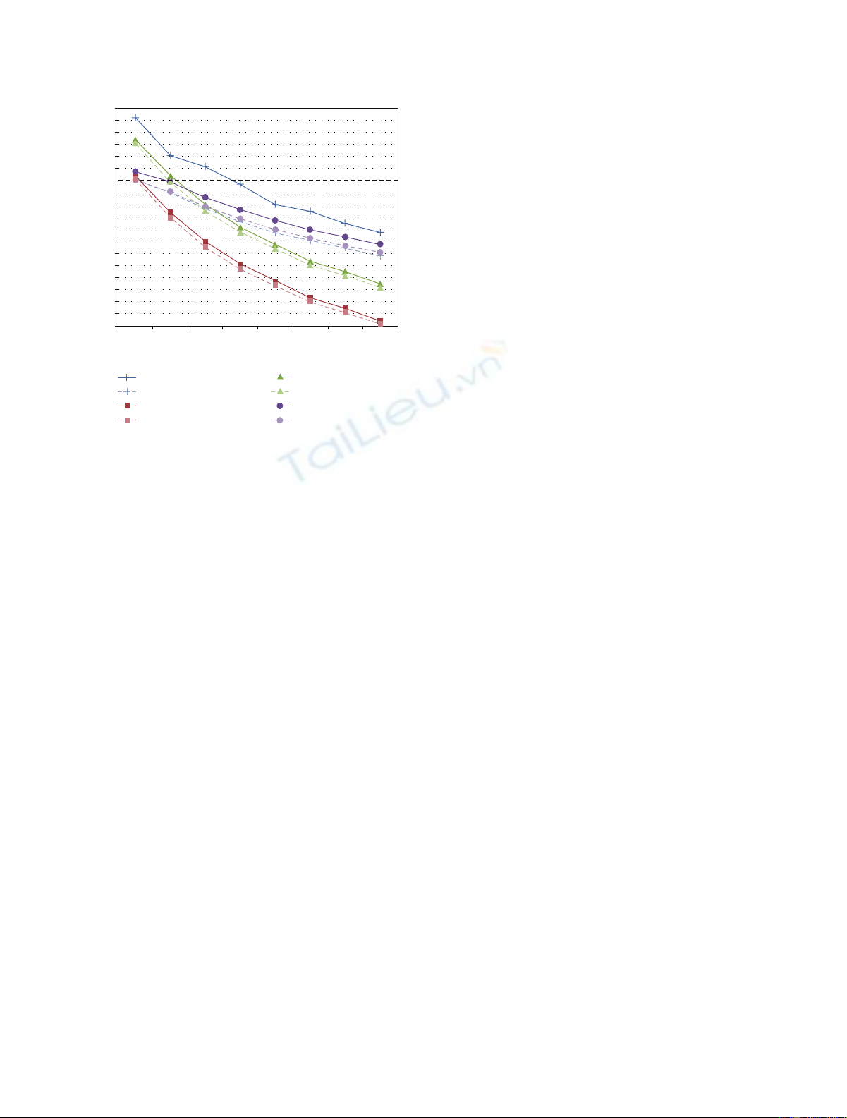
Figure 1: Results for the different HNR estimation methods. HNRY
(in triangles) is the original formula in [9], HNRC (squares) the
pulse number correction in [12], HNRS (plus signs) the shimmer
correction proposed here (using known pulse amplitudes), and
HNRSr (circles) the shimmer correction using estimated pulse
amplitudes. Dashed lines represent results with AWGN; solid lines
and apostrophes represent vocal tract filtered AWGN. Horizontal
dashed line at 30 dB represents true HNR.
The discrete implementation of (28)wasperformedby
setting a sampling frequency of 22050 Hz, a fundamental
frequency of 150 Hz (yielding 147 samples per period), and
M=300, to produce an approximate of 2 seconds of
synthesized voice. The h(t) was obtained as the impulse
response of a five formant all-pole filter, with the same
parameters used in [12,19,21,22]. The glottal flow was
generated using a rising time of 0.33T0and a falling time
of 0.09T0; the values which resulted in the most natural-
sounding synthesis in [23].
The shimmer was controlled by changing the value of
each pulse amplitude ki, obtained as ki=1+vi,whereviis a
random real value, uniformly distributed in the interval ±vm.
Eight levels of shimmer were synthesized, using values of vm
from 0% to 47.6% in steps of 6.8%, measured in percent of
the unaltered amplitude k=1, the same values as in [12,21].
The estimates of HNR calculated were the original
ensemble average formula by Yumoto given in (4), the
correction for any number of pulses given in (5), and
the removal of shimmer effects given by (27). The three
HNR estimates were calculated using first the known pulse
durations and amplitudes, and then using the positions given
by a well-known PDA (the superresolution approach from
Medan et al. [19]), and the amplitudes were calculated with
Milenkovic’s formula [20] using the procedure described in
[21].
A base level of noise was added to the signal, to avoid
values near to zero in the denominator of HNRYum in (4).
The variance of the noise added was chosen to produce an
actual HNR =1000 (30 dB). Two types of noise were added:
AWGN, in conformity with the assumptions of uncorrelated
noise made on deriving (27), and a vocal tract filtered
version, having some level of correlation which is most likely
the case in radiated signals.
The HNR estimates were found for ensembles of two
consecutivepulses(N=2) in the synthesized signals, and
the overall HNR was found as the average of these pairwise
HNR’s.
5. Results and Discussion
The average value for 100 realizations of the random
variables involved (noise and shimmer) was found for each
HNR estimation variant on each shimmer level. It is relevant
to note that the PDA detected the pulse positions without
any error (not even a sample), for all realizations and all
levels of shimmer. For this reason, (4)and(5) produced the
same results using both the known and the detected pulse
positions. Equation (27)produceddifferent results since it
involves also the calculation of the amplitude ratios among
pulses, which produced results different to the values used in
the synthesis.
The results for the different methods facing both noise
types are shown in Figure 1, and the discussion below is
first centered in the AWGN and later in the effect of the
correlation present in the vocal tract filtered noise.
AW G N . For the zero-shimmer level the results are as
predicted: the original approach (HNRY) overestimates the
actual HNR (30 dB), while the corrected approaches produce
adequate and equivalent results. When shimmer appears,
HNRC begins to fall in parallel with HNRY, while both
approaches considering shimmer, HNRS and HNRSr, show
superior performance, with their values less affected by the
increasing levels of shimmer.
Two relevant facts are as follows.
(i) Shimmer-corrected approaches (HNRS and HNRSr)
are nevertheless deteriorated by the shimmer level.
(ii) There is a better performance of HNRSr in compari-
son with HNRS, in spite of using estimated values for
the pulse amplitudes.
Both facts can be explained by the presence, in any pulse
of the signal, of the decaying tails of previous pulses. This
summation of tails adds differences to the pulses, interpreted
as noise in the model and causing a reduction in the
calculated HNR as the introduced shimmer increases. On
the other hand, the summation of tails in one pulse is
not completely uncorrelated with the summation of tails in
the other. For this reason, the estimation of relative pulse
amplitudes, based in the assumption of uncorrelated noise,
produces amplitudes with an overestimation of the signal
component, yielding a higher HNRSr than HNRS.
It is to be expected that in the presence of jitter HNRSr
will perform worse, since pulse tails would not always be
aligned with the adjacent pulse, and the correlation should


![Báo cáo seminar chuyên ngành Công nghệ hóa học và thực phẩm [Mới nhất]](https://cdn.tailieu.vn/images/document/thumbnail/2025/20250711/hienkelvinzoi@gmail.com/135x160/47051752458701.jpg)


%20--%3e%3cdefs%3e%3cstyle%3e%20.st0%20{%20fill:%20%23fff;%20}%20.st1%20{%20fill:%20%237800fa;%20}%20%3c/style%3e%3c/defs%3e%3cpath%20class='st1'%20d='M117.78,12.18H43.11c2.9,3.47,4.65,7.94,4.65,12.82,0,5.6-2.3,10.66-6.01,14.29h76.02l7.22-13.56-7.22-13.56Z'/%3e%3cg%3e%3cpath%20class='st0'%20d='M53.58,26.17h-.59v-1.46h.59v-4.96h2.83c1.78,0,2.67.94,2.67,2.82v5.76c0,1.87-.89,2.81-2.67,2.81h-2.83v-4.96ZM55.36,21.37v3.34h1.1v1.46h-1.1v3.34h1.01c.61,0,.91-.37.91-1.1v-5.93c0-.74-.3-1.1-.91-1.1h-1.01Z'/%3e%3cpath%20class='st0'%20d='M65.99,31.14h-1.8l-.31-2.07h-2.19l-.31,2.07h-1.64l1.82-11.39h2.62l1.82,11.39ZM65.28,18.04c-.25.46-.51.77-.75.94-.21.15-.47.22-.79.22-.26,0-.57-.07-.92-.22l-.38-.15c-.14-.05-.26-.07-.37-.07-.3,0-.53.18-.71.54l-.91-.68c.25-.46.51-.77.75-.94.21-.14.48-.21.79-.21.26,0,.57.07.92.21l.38.15c.14.05.26.07.37.07.3,0,.53-.18.71-.54l.91.68ZM61.91,27.52h1.73l-.87-5.76-.87,5.76Z'/%3e%3cpath%20class='st0'%20d='M74.53,26.89v1.52c0,1.91-.89,2.86-2.67,2.86s-2.67-.95-2.67-2.86v-5.93c0-1.91.89-2.86,2.67-2.86s2.67.95,2.67,2.86v1.11h-1.69v-1.22c0-.75-.31-1.12-.93-1.12s-.93.37-.93,1.12v6.15c0,.74.31,1.11.93,1.11s.93-.37.93-1.11v-1.63h1.69Z'/%3e%3cpath%20class='st0'%20d='M81.4,31.14h-1.8l-.31-2.07h-2.19l-.31,2.07h-1.64l1.82-11.39h2.62l1.82,11.39ZM75.9,19.2l1.52-1.91h1.71l1.51,1.91h-1.61l-.76-.95-.75.95h-1.61ZM77.32,27.52h1.73l-.87-5.76-.87,5.76ZM83.1,15.99l-1.76,1.91h-1.26l1.17-1.91h1.86Z'/%3e%3cpath%20class='st0'%20d='M84.86,19.75c1.78,0,2.67.94,2.67,2.82v1.48c0,1.87-.89,2.81-2.67,2.81h-.85v4.28h-1.79v-11.39h2.64ZM84.01,21.37v3.86h.85c.58,0,.87-.36.87-1.08v-1.71c0-.71-.29-1.07-.87-1.07h-.85Z'/%3e%3cpath%20class='st0'%20d='M93.51,19.75c1.78,0,2.67.94,2.67,2.82v1.48c0,1.87-.89,2.81-2.67,2.81h-.85v4.28h-1.79v-11.39h2.64ZM92.66,21.37v3.86h.85c.58,0,.87-.36.87-1.08v-1.71c0-.71-.29-1.07-.87-1.07h-.85Z'/%3e%3cpath%20class='st0'%20d='M98.8,31.14h-1.79v-11.39h1.79v4.88h2.03v-4.88h1.83v11.39h-1.83v-4.88h-2.03v4.88Z'/%3e%3cpath%20class='st0'%20d='M105.36,24.55h2.46v1.62h-2.46v3.34h3.09v1.63h-4.88v-11.39h4.88v1.63h-3.09v3.18ZM108.17,17.29l-1.76,1.91h-1.26l1.17-1.91h1.86Z'/%3e%3cpath%20class='st0'%20d='M112.2,19.75c1.78,0,2.67.94,2.67,2.82v1.48c0,1.87-.89,2.81-2.67,2.81h-.85v4.28h-1.79v-11.39h2.64ZM111.35,21.37v3.86h.85c.58,0,.87-.36.87-1.08v-1.71c0-.71-.29-1.07-.87-1.07h-.85Z'/%3e%3c/g%3e%3ccircle%20class='st1'%20cx='25'%20cy='25'%20r='20'/%3e%3cpath%20class='st0'%20d='M32.78,19.27c2.92,0,4.43,2.55,5.28,5.33l.71,2.17c.14.38-.33.75-.71.75h-5.61c.19-.33.24-.71.09-1.08l-.75-2.45c-.43-1.32-.99-2.64-1.79-3.77.75-.57,1.65-.94,2.78-.94h0ZM25,18.38c3.25,0,4.9,2.78,5.89,5.89l.76,2.45c.14.42-.33.8-.8.8h-11.69c-.42,0-.94-.38-.8-.8l.75-2.45c.99-3.11,2.64-5.89,5.89-5.89h0ZM25,11.35c1.74,0,3.11,1.37,3.11,3.11s-1.37,3.11-3.11,3.11-3.11-1.41-3.11-3.11,1.41-3.11,3.11-3.11h0ZM17.27,19.27c1.08,0,1.98.38,2.73.94-.8,1.13-1.37,2.45-1.74,3.77l-.8,2.45c-.14.38-.05.75.09,1.08h-5.56c-.42,0-.9-.38-.75-.75l.71-2.17c.9-2.78,2.41-5.33,5.33-5.33h0ZM17.27,12.91c1.51,0,2.78,1.27,2.78,2.83s-1.27,2.83-2.78,2.83-2.83-1.27-2.83-2.83,1.27-2.83,2.83-2.83h0ZM32.78,12.91c1.56,0,2.78,1.27,2.78,2.83s-1.23,2.83-2.78,2.83-2.83-1.27-2.83-2.83,1.27-2.83,2.83-2.83h0ZM27.07,28.56v.09c0,.57-.24,1.08-.61,1.46h0v.05c-.38.33-.9.57-1.46.57s-1.08-.24-1.46-.61h0c-.38-.38-.61-.9-.61-1.46v-.09h1.41v.09c0,.19.05.38.19.47v.05c.09.09.28.19.47.19s.38-.09.47-.19v-.05c.14-.09.24-.28.24-.47t-.05-.09h1.41ZM30.99,28.56v.09c0,1.65-.66,3.16-1.74,4.24-1.08,1.08-2.59,1.79-4.24,1.79s-3.16-.71-4.24-1.79l-.05-.05c-1.04-1.08-1.7-2.55-1.7-4.2v-.09h1.41v.09c0,1.27.47,2.4,1.27,3.25h.05c.85.85,1.98,1.37,3.25,1.37s2.4-.52,3.25-1.37c.85-.8,1.37-1.98,1.37-3.25v-.09h1.37ZM34.99,28.56v.09c0,2.78-1.13,5.28-2.92,7.07-1.79,1.79-4.29,2.92-7.07,2.92s-5.23-1.13-7.07-2.92c-1.79-1.79-2.92-4.29-2.92-7.07v-.09h1.41v.09c0,2.4.94,4.53,2.5,6.08,1.56,1.56,3.72,2.5,6.08,2.5s4.52-.94,6.08-2.5c1.56-1.56,2.5-3.68,2.5-6.08v-.09h1.41Z'/%3e%3c/svg%3e)