Nguyễn Công Phương
CONTROL SYSTEM DESIGN
Stability in the Frequency Domain
Contents
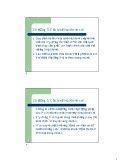
Introduction
I. II. Mathematical Models of Systems III. State Variable Models IV. Feedback Control System Characteristics V. The Performance of Feedback Control Systems VI. The Stability of Linear Feedback Systems VII. The Root Locus Method VIII.Frequency Response Methods IX. Stability in the Frequency Domain X. The Design of Feedback Control Systems XI. The Design of State Variable Feedback Systems XII. Robust Control Systems XIII.Digital Control Systems
sites.google.com/site/ncpdhbkhn
2
Stability in the Frequency Domain
1. Mapping Contours in the s – Plane 2. The Nyquist Criterion 3. Relative Stability and the Nyquist Criterion 4. Time – Domain Performance Criteria in the
Frequency Domain 5. System Bandwidth 6. The Stability of Control Systems with Time
Delays
7. PID Controllers in the Frequency Domain 8. Stability in the Frequency Domain Using
Control Design Software
sites.google.com/site/ncpdhbkhn
3
Ex. 1
Mapping Contours in the s – Plane (1)
jv
jw
s – plane
( )F s
D
2j
F(s) – plane A
2j
D
A
1j
1j
s
2-
1-
1
2
2-
1-
1
2
u
0 1j
0 1j
B
C
- -
B
2j
2j
C
+
1
+
=
+
w
=
- -
= + u
jv
F s
s= ( ) 2
1
s 2(
j
+ ) 1
s (2
+ + 1)
w 2j
s 2 w 2
fi
=
=
s
+
w
+ + s (2 1)
w (2 )
j
· + + (2 1 1)
· = + (2 1) 3
j
2
= u = v j
j 1
= + FA u
j · + +
= jv = -
fi
j 1
j
[2 ( 1)] 3
j
2
= + 1 = - 1 = -
= B =
(2 1 1) - + +
fi · -
sA B s C
j 1
1
j
2
- fi · · - -
1 = - + 1
F C F = D
j 1
[2 ( 1) 1] - + + [2 ( 1) 1]
= - j [2 ( 1)] · = - + j
1
j
2
s D s
F
(2 1) sites.google.com/site/ncpdhbkhn
4
fi ·
Ex. 2
Mapping Contours in the s – Plane (2)
=
F s ( )
s +
s
2
A
D
D
s-plane F(s)-plane 1.5 1.5
1 1
A
v
0.5 0.5
j
j
B
w 0 0
-0.5 -0.5
C
C
B
-1 -1
sites.google.com/site/ncpdhbkhn
5
-1.5 -1.5 -2.5 -2.5 -2 -1.5 -1 -0.5 0 0.5 1 1.5 -2 -1.5 -1 0 0.5 1 1.5 s -0.5 u
Mapping Contours in the s – Plane (3)
s-plane F(s)-plane
+
2 2
F s
s= ( ) 2
1 1
v
1
j
j
w 0 0
-1 -1
-2 -2
0 -2 -1 -1 -2 1 2 3 0 1 2 3 s u
Cauchy’s theorem: If a contour Γs in the s-plane encircles Z zeros and P poles of F(s) and does not pass through any poles or zeros of F(s) and the traversal is in the clockwise direction along the contour, the corresponding contour ΓF in the F(s)-plane encircles the origin of the F(s)-plane N = Z – P times in the clockwise direction.
F(s)-plane s-plane 1.5 1.5
1 1
v
j
jw
0.5 0.5
0 0
=
F s ( )
s
-0.5
s -0.5 + 2 -1
-1
6
-1.5 -1.5 -2 -1 0 1 -1 0 1 s u -2 sites.google.com/site/ncpdhbkhn
Ex. 3
Mapping Contours in the s – Plane (4)
=
F s ( )
s + 0.5
s
F(s)-plane s-plane 0.15 6
0.1 4
v
2 0.05
j
j
w 0 0
-2 -0.05
-4 -0.1
If a contour Γs in the s-plane encircles Z zeros and P poles of F(s) and does not pass through any poles or zeros of F(s) and the traversal is in the clockwise direction along the contour, the corresponding contour ΓF in the F(s)-plane encircles the origin of the F(s)-plane N = Z – P times in the clockwise direction.
sites.google.com/site/ncpdhbkhn
7
-6 -6 -4 -2 0 2 4 6 0.9 0.95 1 1.1 1.15 s 1.05 u
Ex. 2
=
Mapping Contours in the s – Plane (5) =
f
=
F s ( )
= ( ) F s
F s ( )
F s ( )
f (
)
z
p
s +
+ +
s
2
s s
z p
If a contour Γs in the s-plane encircles Z zeros and P poles of F(s) and does not pass through any poles or zeros of F(s) and the traversal is in the clockwise direction along the contour, the corresponding contour ΓF in the F(s)-plane encircles the origin of the F(s)-plane N = Z – P times in the clockwise direction.
F(s)-plane
s-plane
1.5
1.5
1
1
f
f-
f
0.5
0.5
z
z
p
v
— — -
j
0
0
j
f
p
-0.5
-0.5
-1
-1
-1.5
-1.5
-2.5
-2
-1.5
-1
-0.5
0
0.5
-2
-1.5
-1
0
0.5
1.5
1
1.5
w
-0.5 u
-2.5 sites.google.com/site/ncpdhbkhn
1 8
s
Stability in the Frequency Domain
1. Mapping Contours in the s – Plane 2. The Nyquist Criterion 3. Relative Stability and the Nyquist Criterion 4. Time – Domain Performance Criteria in the
Frequency Domain 5. System Bandwidth 6. The Stability of Control Systems with Time
Delays
7. PID Controllers in the Frequency Domain 8. Stability in the Frequency Domain Using
Control Design Software
sites.google.com/site/ncpdhbkhn
9
The Nyquist Criterion (1)
• F(s) = 1 + L(s) = 0
jw
s – plane
r fi
• A feedback system is stable if and only if the contour ΓL in the L(s) – plane does not encircle the (–1, 0) point when the number of poles of L(s) in the right – hand s – plane is zero (P = 0).
0
s
•
¥
s
Nyquist contour
(when the number of poles of L(s) in the right – hand s – plane is other than zero) A feedback system is stable if and only if, for the contour ΓL , the number of counterclockwise encirclements of the (–1, 0) point is equal to the number of poles of L(s) with positive real parts.
sites.google.com/site/ncpdhbkhn
10
G
The Nyquist Criterion (2)
Ex. 1
( )R s
( )Y s
t
1 + s
1 1st + 1
1 1st + 2
1 + s 1
2
=
( )-
T s ( )
+
1
K
t
1 1 + s
1
. t 1 1 + s 1
2
K
= ( ) L s
L s ( )
K
K
A feedback system is stable if and only if the contour ΓL in the L(s) – plane does not encircle fi + 1 the (–1, 0) point when the number of poles of L(s) in the right – hand s – plane is zero (P = 0).
t
t
1 + s
. t 1
1 + s
1
. t 1 1 = = + 0 1 + 1 s
1 + s
. t 1
1
2
1
2
=
w j
w
fi
jv
jw
=
=
w L j (
)
0
s – plane
w
fi ¥
A
=
s
w fi
fi ¥
sA LA sB
r fi
=
=
s s (
)
0
L
s
¥ fi ¥ ¥
LB
D
,C
A
, B
D 0
B s
0
u
=
w j
fi ¥
sC
w =
1 t
1 t
0
1
2
=
=
0
)
w
fi - ¥ - -
fi - ¥
s
C
w w L j ( = + 0
j
=
0 =
L
(0)
K
L(s) – plane
LC sD LD
sites.google.com/site/ncpdhbkhn
11
G
The Nyquist Criterion (3)
Ex. 2
jw
s – plane
=
D
L s ( )
K st + (
s
1)
r fi
C
=
B
w j
sA
w
<
¥
w 0,
0
E s
0
fi
e
1 t
A
=
w L j (
)
LA
w
<
-
w 0,
0
fi
s
F
=
+
K j
w j
(
tw )(
1)
w
<
G
w 0,
0
= -
fi
+ ¥ t K
j
t K 2
K 2
2
+
+
t w 2
j wt w
1
(
1)
= -
w
<
-
w 0,
0
Cauchy’s theorem: If a contour Γs in the s-plane encircles Z zeros and P poles of L(s) and does not pass through any poles or zeros of L(s) and the traversal is in the clockwise direction along the contour, the corresponding contour ΓF in the L(s)-plane encircles the origin of the L(s)-plane N = Z – P times in the clockwise direction. sites.google.com/site/ncpdhbkhn
12
fi
K = 2, t = 1
The Nyquist Criterion (4)
Ex. 2
jw
A
20
s – plane
=
D
L s ( )
15
s
1)
10
r fi
C
= -
K st + ( + ¥ t K
j
LA
B
v
j
¥ 5
B
,D F
E s
0
0
e
=
s
1 t
s
sB
0
A
- -5 fi
s
K
F
=
=
s (
L
)
B L
s
0
C
+
s s (
1)
s
0
-10 G -15 fi fi -20
= ¥
=
= -
0 10 20 u
w j
w L j (
)
t K
j
sC
w
>
= C L
w
>
w 0,
0
w 0,
= 0
+
K j
w j
(
tw )(
1)
>
w
w 0,
0
=
=
=
fi - ¥ fi fi fi
w j
w L j (
)
0
sD
w
w
= D L
+
w j
(
tw )(
1)
w
=
=
=
fi fi ¥ fi ¥ fi ¥
w j
)
0
w L j (
sF
w
w
= F L
+
(
tw )(
1)
K j K j
w j
w
sites.google.com/site/ncpdhbkhn
13
fi fi - ¥ fi - ¥ fi - ¥
The Nyquist Criterion (5)
jv
jw
s – plane
A
=
L s ( )
+
+
K t 1)(
t (
s
1)
s
w fi
1
2
r fi
D
A, B,C
D 0
B s
0
u
•
¥ ¥
w =
0
1 t
1 t
1
2
- -
s
C
K = 2, t = 1
It is sufficient to construct the contour ΓL for the frequency range 0<ω<∞ in order to investigate the stability.
20
jw
A
s – plane
15
D
10
G
r fi
C
5
B
v
j
0
B
,D F
• The magnitude of L(s) as s = rejϕ and r →∞ will normally approach zero or a constant.
E s
0
¥
e
-5
1 t
A
-10
-
=
-15
s
F
L s ( )
C
1)
s
-20
K st + ( sites.google.com/site/ncpdhbkhn
14
0
10
20
u
G
jw
s – plane
D
The Nyquist Criterion (6)
r fi
¥
Ex. 3
C
B
=
L s ( )
E s
0
+
+
e
K t 1)(
t (
s
1)
s 1
2
1 t
A
=
w L j (
)
-
+
s
s K wt + 1)(
w wt j (
j
j
1)
F
1
2
2
G
K
t (
)
1 2
=
jK +
+ t 1 + 1
) 2 w t 2 (
w (1/ + wtt 2 ) 2
wtt )(1 4 2 2 2 1
t 2 1
- - -
=
p
[
wt 1 tan (
)
wt 1 tan (
)
/ 2]
1
2
2
2
w t 4
wtt 2
K +
+
- - — - - -
(
w 2 )
(1
)
t 1
2
1 2
=
p
-
C
w j
= )
(
/ 2)
s
= C L
w
>
w 0,
0
w
2
2
w lim ( L j w 0
lim 0
w t 4
wtt 2
K +
+
(
w 2 )
(1
)
t 1
2
1 2
K
=
fi — - fi fi fi -
w j
= )
lim
p ( 3 / 2)
D s
= D L
w
3
w lim ( L j w
w
ttw 1 2
sites.google.com/site/ncpdhbkhn
15
fi — - fi ¥ fi ¥ fi ¥
jw
s – plane
D
The Nyquist Criterion (7)
r fi
¥
Ex. 3
C
B
=
L s ( )
E s
0
+
+
e
K t 1)(
t (
s
1)
s
s 1
2
1 t
A
K
=
p
p
-
C
(
/ 2);
( 3 / 2)
L
= D L
K 0
s
F
2
— - — - G ¥
)
1 2
=
j
w L j (
)
+
w t 2
t ( +
wtt )(1 +
K = 1, t
= 5, t
= 5
(
1
K + t 1
w (1/ wtt 2 (
)
K t 2 1
+ t 2 1 + wtt 2 ) 2
w t 4 2 2 2 1
) 4 2 2 2 1
2 2
2 1
1
2
+ 6
2
- - -
1 2
w L j Im{ (
= fi )} 0
0
4
)(1 +
K (1/ + w t 2 (
1
w t 2 1
wtt + wtt 2 ) 2
) = 4 2 2 2 1
2
-
w =
L w Re( )
=
tt K 1 2 + t
t
= 1 tt 1 2
v
2
1
1 tt 1 2
j
0
-2
t
- fi fi
+ t 1
2
1
K
-4
tt K 1 2 + t
t
tt
2
1
1 2
-6
-6
-4
-2
0
2
4
sites.google.com/site/ncpdhbkhn
16
u
- fi ‡ - fi £
The Nyquist Criterion (8)
Ex. 3
t
2
=
K
L s ( )
+
+
K t 1)(
t (
s
1)
s
+ t 1 tt 1 2
s 1
2
K = 2, t
= 1, t
= 1
K = 3, t
= 1, t
= 1
K = 1, t
1
2
1
2
= 1, t 1
= 1 2
1.5
1.5
1.5
1
1
1
0.5
0.5
0.5
v
v
v
j
j
j
0
0
0
-0.5
-0.5
-0.5
-1
-1
-1
-1.5
-1.5
-1.5
-2
-1
0
1
-2
-2
-1
0
1
-1
0
1
u
u
u
sites.google.com/site/ncpdhbkhn
17
£
jw
s – plane
D
The Nyquist Criterion (9)
r fi
¥
Ex. 4
C
B
=
L s ( )
E s
0
2
+
e
K st (
s
1 t
A
-
=
=
w L j (
)
p [
wt 1 tan (
)]
2
4
2
6
w
+
w
K + t w
s
wt (
1)
1) K j
F
=
C
w j
s
w
>
- — - - G -
2
w 0,
0
1.5
fi
= w L j )
p (
)
= C L
w
lim ( w 0
lim 0
K w 2
1
0.5
=
w j
D s
w
fi — - fi fi
v
j
0
K
p
fi ¥
w = L j )
lim
( 3 / 2)
= D L
3
lim ( w
w
-0.5
tw
-1
f j
=
e
e
B s
e
fi — - fi ¥ fi ¥
0
-1.5
fi
f j
2
e L e
f = j )
e
= B L
-2 -2.5
-2
-1.5
-1
-0.5
0
0.5
1
1.5
2
lim ( e 0
lim e 0
K e 2
u
sites.google.com/site/ncpdhbkhn
18
- fi fi fi
The Nyquist Criterion (10)
2.5
2
( )Y s
s – plane
Ex. 5 ( )R s
1.5
jw D
1K
1
1 s
1 1s -
( )-
0.5
r fi
C
v
j
0
B
-0.5
E s
0
e 1
-1
1K
=
A
L s ( )
-1.5
¥
K 1 s s (
1)
-2
-
s
F
-2.5
-3
-2
-1
0
u
G
Ex. 6
2
s – plane
( )Y s
( )R s
1.5
jw D
1K
1
1 s
1 1s -
( )-
r fi
C
( )-
0.5
2K
v
B
j
0
-0.5
E s
¥
0
e 1
1 K
2
-1
+
1)
A
=
L s ( )
-1.5
-
K K s ( 2 1 s s (
1)
-2
s
F
-5
-4
-3
-2
0
sites.google.com/site/ncpdhbkhn
-1 19
u
- G
The Nyquist Criterion (11)
2
s – plane
( )Y s
1.5
Ex. 6 ( )R s
jw D
1K
1
1 s
1 1s -
( )-
r fi
C
( )-
0.5
2K
v
B
j
0
-0.5
E s
¥
0
e 1
1 K
2
-1
+
1)
A
=
L s ( )
-1.5
-
( K K s 1 2 s s (
1)
-2
s
F
-5
-4
-3
-2
-1
0
u
2
2
+
- G
(
K
)
K
1) +
= w ) L j (
+ 2 2
2 2
w K 1 w
w
w K 1 j w
+ 4
w (1 + 4
w K K j ( 1 2 w w ( j j
- - fi -
w w K
2
w K 1
2 ) = fi
w =
w L j Im{ (
= fi )} 0
0
2 2
1) = 1) (1 4
w
w +
1 K
2
2
-
1)
=
= -
Re{ (
w L j
)}
2
K K 1
2
w
4
+ 2 2
= 1/
K
2
w K 1 w
( K + w
2
w
= 1/
K
2
= - + = fi
-
If
1
= 1
+ Z N P
1 1 0
stable
K K 1
< - 2
> fi K K 1 2
sites.google.com/site/ncpdhbkhn
20
- fi
The Nyquist Criterion (12)
2
s – plane
( )Y s
1.5
Ex. 6 ( )R s
jw D
1K
1
1 s
1 1s -
( )-
r fi
C
( )-
0.5
2K
v
B
j
0
-0.5
E s
¥
0
e 1
1 K
2
-1
A
K K >
1
-1.5
2
1
-
-2
s
F
-5
-4
-3
-2
-1
0
K
K
u K = 1, K = 0.5, K K 1 2 1
= 0.5 2
K = 3, K = 0.5, K 1 2 1
= 1.5 2
= 1 K = 2, K = 0.5, K 2 1 2 1
2
2
2
1
1
1
v
v
v
j
j
j
0
0
0
-1
-1
-1
-2
-2
-2
-4
-2
0
-4
0
-2
-4
-2
0
u
u
u
sites.google.com/site/ncpdhbkhn
21
G
Stability in the Frequency Domain
1. Mapping Contours in the s – Plane 2. The Nyquist Criterion 3. Relative Stability and the Nyquist Criterion 4. Time – Domain Performance Criteria in the
Frequency Domain 5. System Bandwidth 6. The Stability of Control Systems with Time
Delays
7. PID Controllers in the Frequency Domain 8. Stability in the Frequency Domain Using
Control Design Software
sites.google.com/site/ncpdhbkhn
22
Ex. 1
= 1; t 1
= 1 2
0.5
=
L s ( )
+
+
t
Relative Stability and the Nyquist Criterion (1) K t 1)(
1)
s
t (
s
s 1
=
w L j (
)
+
2 K t w + 1)(
wt w j (
j
j
1)
0
1
2
(
)
2
v
=
j
+
-
w t 4
t + 1 ttw 2
w t 2 K w + 2 )
(
2 2 )
2
t 1
1 2
2
-
w
Ktt 1 2 t+ t
-0.5
K
)
1
2
j
+
w t 4
(
(1 ttw (1 + w 2 )
1 2 ttw 2 (1
2 2 )
t 1
2
1 2
2
w
- - -
)
K
K = 2.5 K = 1.2 K = 0.3
w L j Im{ (
= fi )} 0
0
w t 4
+
-
ttw (1 w + 2 )
1 2 ttw 2 (1
(
= 2 2 )
t 1
2
1 2
-1 -1.5
-1
-0.5
0
u
w =
-
1 tt 1 2
tt
fi
(
)
2
1 2
=
=
w L j Re{ (
)}
w
tt
= 1/
1 2
t + 1 ttw 2
w t 4
+
- -
w t 2 K w + 2 )
(1
(
2 2 )
t tt
w
2
t 1
1 2
K + 1
2
t = 1/
1 2
sites.google.com/site/ncpdhbkhn
23
-
Relative Stability and the Nyquist Criterion (2)
= 1; t 1
= 1 2
0.5
Phase difference before instability
0
a
v
j
d
=
=
Gain margin
20log
MG
-0.5
1 d
K = 2.5 K = 1.2 K = 0.3
a
Phase margin
= F = M
-1 -1.5
-1
-0.5
0
u Gain difference before instability
sites.google.com/site/ncpdhbkhn
24
t
Ex. 2
0.5
Relative Stability and the Nyquist Criterion (3) =
Given
L s ( )
+
+
6 + 2
2)(
2
s
2)
s s ( Find its gain & phase margin?
0
=
a
w L j (
)
Phase difference before instability
w
+
+
6 + 2
w j
(
w 2)(
2
j
2)
v
j
2
d
w
-
=
2
-
w
-0.5
16(1
24(1 + w 2 2 )
2 2 )
2
) w (6 w
- -
j
2
w
16(1
w 6 (6 w + 2 2 )
) w (6
2 2 )
2
w
- - - -
-1 -1.5
-1
-0.5
0
=
= w
L Im{ }
= fi 0
2.45 rad/s
2
w
-
2 2 )
16(1
w 6 (6 + w 2 2 )
) w (6
u Gain difference before instability
2
w
- -
=
=
=
d
0.3
L w Re{ }
=
2
2.45
-
w
24(1 + w 2 2 )
) w (6
16(1
2 2 )
=
w
2.45
=
=
=
=
Gain margin
20log
20log
10.46 dB
MG
1 d
1 0.3
sites.google.com/site/ncpdhbkhn
25
- -
Ex. 2
0.5
Relative Stability and the Nyquist Criterion (4) =
Given
L s ( )
+
6 + 2
+
2)
s
2
2)(
0
=
1
)
a
Phase difference before instability
2
2
w
v
j
2
d
w
24(1 + w 2 2 )
) w (6
16(1
2 2 )
s s ( Find its gain & phase margin? L jw (
2
-0.5
2
- fi - -
w
w =
+
=
1.253 rad/s
1
2
w
16(1
w 6 (6 + w 2 2 )
) w (6
2 2 )
- fi - -
w L j (
)
atan
w
= = 1.253
Im{ } L L Re{ }
w
-1 -1.5
-1
-0.5
0
= 1.253
2
w
fi —
u Gain difference before instability
2
w
-
16(1
2 2 )
=
= -
atan
o 112.3
w
- -
2
w
-
16(1
w 6 (6 w + 2 2 ) 24(1 w + 2 2 )
) w (6 2 ) w (6
2 2 )
w
= 1.253
o
= F =
= -
a
- -
Phase margin
o 112.3
= o ( 180 )
67.7
M
sites.google.com/site/ncpdhbkhn
26
fi - -
Relative Stability and the Nyquist Criterion (5)
= 1; t 1
= 1 2
0.5
=
=
Gain margin
20log
MG
1 d
a
Phase difference before 0 instability
v
j
d
-0.5
The gain margin is the increase in the system gain when phase = –180° that will result in a marginally stable system with intersection of the –1 + j0 point on the Nyquist diagram.
K = 2.5 K = 1.2 K = 0.3
a
Phase margin
= F = M
-1 -1.5
-1
-0.5
0
u Gain difference before instability
The phase margin is the amount of phase shift of the L(jωt) at unity magnitude that will result in a marginally stable system with intersection of the – 1 + j0 point on the Nyquist diagram.
sites.google.com/site/ncpdhbkhn
27
t
Ex. 2
=
=
w
=
Gain margin
10.46 dB,
2.45 rad/s
MG
Relative Stability and the Nyquist Criterion (6) =
Given
L s ( )
+
+
6 + 2
2)(
2
s
2)
= w
Phase margin
o 67.7 ,
1.253 rad/s
= F = M
s s ( Find its gain & phase margin?
Bode Diagram
5
0
)
-5
MG
-10
B d ( e d u t i n g a M
-15
-20
1.5
2
2.5
3
3.5
4
1
-25 -45
-90
) g e d (
-135
M
e s a h P
-180
-225
1
1.5
2
2.5
3
3.5
4
Frequency (rad/s)
sites.google.com/site/ncpdhbkhn
28
F
Ex. 3
Relative Stability and the Nyquist Criterion (7)
=
=
Compare
.
L s ( ) 1
L s & ( ) 2
2
+
+
1 +
1 1)(0.2
1)
s
s s (
s s (
1)
Bode Diagram
10
0
2MG
)
1MG
-10
-20
B d ( e d u t i n g a M
-30
G>
G M
M
2
-40 -90
1 > F 1 M
M
2
L 1 L 2
-135
F
1M
-180
F
2M
) g e d ( e s a h P
-225
-270
0.5
0.6
0.7
0.8
0.9
1
2
3
4
Frequency (rad/s)
sites.google.com/site/ncpdhbkhn
29
F
Relative Stability and the Nyquist Criterion (8)
2
2
o
2 n
=
w
=
w L j (
)
+ z w 4
90
atan
2 n
w 2 n zw +
w w
w w j (
j
2
)
w zw 2
n
n
F = -
— - -
1
o90
atan
M
w zw 2
n
0.9
Exact Linear approximation
0.8
2
2 n
w
+
=
z w 4
1
2 c
2 n
0.7
w w
c
fi -
0.6
, o
i t a r
2
z
0.5
z + - 4 4
z 1 2
i
w w
2 = c 2 n
0.4
g n p m a D
0.3
2
F =
fi
atan
M
0.2
4
z
fi
4+1/
2
0.1
0
0
10
20
30
40
50
70
80
90
100
z
=
z
-
0.01
,
0.7
Phase margin, F
60 ( o ) M
M
sites.google.com/site/ncpdhbkhn
30
F £
Stability in the Frequency Domain
1. Mapping Contours in the s – Plane 2. The Nyquist Criterion 3. Relative Stability and the Nyquist Criterion 4. Time – Domain Performance Criteria in the
Frequency Domain
5. System Bandwidth 6. The Stability of Control Systems with Time
Delays
7. PID Controllers in the Frequency Domain 8. Stability in the Frequency Domain Using
Control Design Software
sites.google.com/site/ncpdhbkhn
31
Time – Domain Performance Criteria in the Frequency Domain (1)
( )R s
( )Y s
( )G s
cG s ( )
)
=
=
w T j (
)
( )-
)
w Y j ( w R j (
) )
)
(
)
j
=
( )H s
= + u
)
(
jv
w w G j G j ( ( ) c w w + ( 1 G j G j ( c M e f w w ( ) w w ( cG j G j )
1.5
)
M =
0.7
M =
1.5
1M =
M
w (
= )
1
w w G j G j ) ( ( c + w w ( G j G j (
)
1
)
c
0.5
2
2
+
=
=
0
2
2
2M =
M =
0.5
u +
v +
+ jv u + + u
jv
1
u
)
(1
v
-0.5
-1
2
2
2
M
2
-1.5
fi
u
= v
-3
-2.5
-2
-1.5
-1
-0.5
0
0.5
1
1.5
2
2.5
+ 2
2
1
M
- 1
M M
sites.google.com/site/ncpdhbkhn
32
fi - -
Time – Domain Performance Criteria in the Frequency Domain (2)
4.5
1
K
1
1M
K
2
2M
4
0.5
3.5
0
3
1M
2.5
v
j
-0.5
e d u t i n g a M
2
2M
-1
1.5
K>
K 1
2
1
-1.5
0.5
1K
2K
-2
0
-2.5
-2
-1.5
-1
-0.5
0
0
0.2
0.4
0.6
0.8
1
1.2
1.4
1.6
1.8
2
u
=
=
Polar plot of w L j ( )
)
(
w KP j (
)
=
w w ( cG j G j )
)
w T j (
Frequency response of w w G j G j ) ( ( ) c + w w ( G j G j (
1
)
c
) 33
sites.google.com/site/ncpdhbkhn
w
Time – Domain Performance Criteria in the Frequency Domain (3)
6
( )R s
( )Y s
f =
o10
( )G s
cG s ( )
( )-
4
f =
o20
( )H s
2
)
f w ( j
)
=
=
=
w
w T j (
)
M e ( )
f =
w Y j ( w R j (
) )
w w G j G j ( ( ) c + w w ( G j G j (
)
1
)
o30
c
1.5
0
M =
0.7
M =
1.5
1M =
f = -
1
o30
0.5
-2
0
2M =
M =
0.5
f = -
o20
-0.5
-4
-1
f = -
o10
-1.5
-6
-4
-3
-2
-1
0
1
2
3
-3
-2.5
-2
-1.5
-1
0
0.5
1
2
2.5
1.5
2
2
2
2
M
-0.5 2 +
= 2
+
2 =
u
v
u
v
+ 1
2
2
1 2
f
1
M
- 1
M M
+ 1 2
1 f 2
1 4
sites.google.com/site/ncpdhbkhn
34
- - -
Ex.
( )R s
( )Y s
( )G s
=
cG s ( )
= ( ) 1
H s
,
cG s G s ( ) ( )
Time – Domain Performance Criteria in the Frequency Domain (4) 0.47 + + 2 s
s s (
1)
( )-
( )H s
Nichols Chart
20
1 dB
15
3 dB
10
6 dB
)
5
i
0
-5
B d ( n a G p o o L - n e p O
-10
-15
-20
-270
-225
-180
-135
-90
Open-Loop Phase (deg)
sites.google.com/site/ncpdhbkhn
35
Stability in the Frequency Domain
1. Mapping Contours in the s – Plane 2. The Nyquist Criterion 3. Relative Stability and the Nyquist Criterion 4. Time – Domain Performance Criteria in the
Frequency Domain 5. System Bandwidth 6. The Stability of Control Systems with Time
Delays
7. PID Controllers in the Frequency Domain 8. Stability in the Frequency Domain Using
Control Design Software
sites.google.com/site/ncpdhbkhn
36
System Bandwidth (1)
Ex. 1
0
=
=
,
T s ( ) 1
T s ( ) 2
-3
T 1 T 2
1 +
s
1
1 + s
5
1
-6
B d
, |
-8
|
l
-10
T g o 0 2
-18
0
0.2
1
2
Step Response
1
0.8
0.6
e d u t i l
p m A
0.4
T 1
0.2
T 2
0
0
2
4
6
8
10
Time (seconds)
sites.google.com/site/ncpdhbkhn
37
w
System Bandwidth (2)
Ex. 2
=
=
,
T s ( ) 1
T s ( ) 2
2
2
+
+
100 + s 10
s
100
s
900
900 + s 30
10
Step Response
1.2
T 1 T 2
T 1 T 2
0 -3
1
-10
0.8
-20
B d , |
|
-30
e d u
t i l
0.6
l
T g o 0 2
p m A
-40
0.4
-50
0.2
-60
0
-70
0
2
0
0.2
0.4
0.6
0.8
1
1.2
1.4
1.6
10
1 10
10
Time (seconds)
sites.google.com/site/ncpdhbkhn
38
w
Stability in the Frequency Domain
1. Mapping Contours in the s – Plane 2. The Nyquist Criterion 3. Relative Stability and the Nyquist Criterion 4. Time – Domain Performance Criteria in the
Frequency Domain 5. System Bandwidth 6. The Stability of Control Systems with Time
Delays
7. PID Controllers in the Frequency Domain 8. Stability in the Frequency Domain Using
Control Design Software
sites.google.com/site/ncpdhbkhn
39
The Stability of Control Systems with Time Delays (1) • Time delay: the time interval between the start of an even at one point in a system and its resulting action at another point in the system.
• A pure time delay, without attenuation:
Gd(s) = e–sT
• A pure time delay does not change the magnitude of the transfer function.
• The Nyquist criterion remains valid for a
system with a time delay.
sites.google.com/site/ncpdhbkhn
40
-
Ex.
+ s
1
sT
e
s
=
e
T s ( )
+
2
1
s
+
+
+
- » -
The Stability of Control Systems with Time Delays (2) 31.5 s 1)[( / 3)
+ / 3 1]
1)(30
s
s
(
s
T 2 T 2
6
4
B d
2
, |
|
0
l
-2
T 0 1 g o 0 2
-4
-0.2
-0.1
0.1
-0.3
10
10
0 10
10
-6 10
-100
With time delay Without time delay
-150
)
o
(
w
-180
without time delay
-200
F f
with time delay
-0.2
-0.1
0.1
10
10
0 10
10
-250 -0.3 10
F
sites.google.com/site/ncpdhbkhn
41
w
Stability in the Frequency Domain
1. Mapping Contours in the s – Plane 2. The Nyquist Criterion 3. Relative Stability and the Nyquist Criterion 4. Time – Domain Performance Criteria in the
Frequency Domain 5. System Bandwidth 6. The Stability of Control Systems with Time
Delays
7. PID Controllers in the Frequency Domain 8. Stability in the Frequency Domain Using
Control Design Software
sites.google.com/site/ncpdhbkhn
42
Ex.
PID Controllers in the Frequency Domain (1) dT s ( )
w
K
( )Y s
( )R s
2 n
g
I
+
+
K
P
K s D
2
+
+
+
K s
t (
s
1)(
s
zw 2
w s
)
n
2 n
g
g
( )-
( )H s
2
(
=
w
L s ( )
K
K
2 n
D
2
g
D +
w
+ t (
/ I + s
s s
) )
s
n
g
o
z =
K = –7000, τ = 5s. Design the PID controller so that GM ≥ 6dB, 30o ≤ ΦM ≤ 60o, rise time Tr < 4s, time to peak TP < 10s. + ( ) / K K s K K P D + zw 2 s 1)( 2 n g = 0.01 30
0.3 +
·
0.6
2.16 0.3 0.6
=
=
< fi 4
0.31
> w n
T r
F = 0.01 M + z 2.16 w
w
n
n +
p
p
·
w
=
0.4
3s,
8s
n
= T r
= T P
= 2
· fi
z
w
2.16 0.3 0.6 = 0.4
1
= 2 0.4 1 0.3
n
43
sites.google.com/site/ncpdhbkhn
- -
PID Controllers in the Frequency Domain (2)
2
Ex. K = –7000, τ = 5s. Design the PID controller so that GM ≥ 6dB, 30o ≤ ΦM ≤ 60o, rise time Tr < 4s, time to peak TP < 10s. + (
=
w
z
=
=
L s ( )
K
K
,
w 0.3,
0.4
2 n
D
n
2
g
w
/ +
D +
+ t (
s
s s
I s
) )
( ) / K K s K K P D zw + 2 s 2 1)( n
n g
g
Bode Diagram
20
10
)
0
B d (
MG
-10
e d u
t i
-20
n g a M
-30
-40 -45
-90
-135
) g e d ( e s a h P
-180
M
-225
-1
10
0 10
1 10
Frequency (rad/s)
sites.google.com/site/ncpdhbkhn
44
F
Stability in the Frequency Domain
1. Mapping Contours in the s – Plane 2. The Nyquist Criterion 3. Relative Stability and the Nyquist Criterion 4. Time – Domain Performance Criteria in the
Frequency Domain 5. System Bandwidth 6. The Stability of Control Systems with Time
Delays
7. PID Controllers in the Frequency Domain 8. Stability in the Frequency Domain Using
Control Design Software
sites.google.com/site/ncpdhbkhn
45
Stability in the Frequency Domain Using Control Design Software
• nyquist • nichols • margin • pade • ngrid
sites.google.com/site/ncpdhbkhn
46


%20--%3e%3cdefs%3e%3cstyle%3e%20.st0%20{%20fill:%20%23fff;%20}%20.st1%20{%20fill:%20%237800fa;%20}%20%3c/style%3e%3c/defs%3e%3cpath%20class='st1'%20d='M117.78,12.18H43.11c2.9,3.47,4.65,7.94,4.65,12.82,0,5.6-2.3,10.66-6.01,14.29h76.02l7.22-13.56-7.22-13.56Z'/%3e%3cg%3e%3cpath%20class='st0'%20d='M53.58,26.17h-.59v-1.46h.59v-4.96h2.83c1.78,0,2.67.94,2.67,2.82v5.76c0,1.87-.89,2.81-2.67,2.81h-2.83v-4.96ZM55.36,21.37v3.34h1.1v1.46h-1.1v3.34h1.01c.61,0,.91-.37.91-1.1v-5.93c0-.74-.3-1.1-.91-1.1h-1.01Z'/%3e%3cpath%20class='st0'%20d='M65.99,31.14h-1.8l-.31-2.07h-2.19l-.31,2.07h-1.64l1.82-11.39h2.62l1.82,11.39ZM65.28,18.04c-.25.46-.51.77-.75.94-.21.15-.47.22-.79.22-.26,0-.57-.07-.92-.22l-.38-.15c-.14-.05-.26-.07-.37-.07-.3,0-.53.18-.71.54l-.91-.68c.25-.46.51-.77.75-.94.21-.14.48-.21.79-.21.26,0,.57.07.92.21l.38.15c.14.05.26.07.37.07.3,0,.53-.18.71-.54l.91.68ZM61.91,27.52h1.73l-.87-5.76-.87,5.76Z'/%3e%3cpath%20class='st0'%20d='M74.53,26.89v1.52c0,1.91-.89,2.86-2.67,2.86s-2.67-.95-2.67-2.86v-5.93c0-1.91.89-2.86,2.67-2.86s2.67.95,2.67,2.86v1.11h-1.69v-1.22c0-.75-.31-1.12-.93-1.12s-.93.37-.93,1.12v6.15c0,.74.31,1.11.93,1.11s.93-.37.93-1.11v-1.63h1.69Z'/%3e%3cpath%20class='st0'%20d='M81.4,31.14h-1.8l-.31-2.07h-2.19l-.31,2.07h-1.64l1.82-11.39h2.62l1.82,11.39ZM75.9,19.2l1.52-1.91h1.71l1.51,1.91h-1.61l-.76-.95-.75.95h-1.61ZM77.32,27.52h1.73l-.87-5.76-.87,5.76ZM83.1,15.99l-1.76,1.91h-1.26l1.17-1.91h1.86Z'/%3e%3cpath%20class='st0'%20d='M84.86,19.75c1.78,0,2.67.94,2.67,2.82v1.48c0,1.87-.89,2.81-2.67,2.81h-.85v4.28h-1.79v-11.39h2.64ZM84.01,21.37v3.86h.85c.58,0,.87-.36.87-1.08v-1.71c0-.71-.29-1.07-.87-1.07h-.85Z'/%3e%3cpath%20class='st0'%20d='M93.51,19.75c1.78,0,2.67.94,2.67,2.82v1.48c0,1.87-.89,2.81-2.67,2.81h-.85v4.28h-1.79v-11.39h2.64ZM92.66,21.37v3.86h.85c.58,0,.87-.36.87-1.08v-1.71c0-.71-.29-1.07-.87-1.07h-.85Z'/%3e%3cpath%20class='st0'%20d='M98.8,31.14h-1.79v-11.39h1.79v4.88h2.03v-4.88h1.83v11.39h-1.83v-4.88h-2.03v4.88Z'/%3e%3cpath%20class='st0'%20d='M105.36,24.55h2.46v1.62h-2.46v3.34h3.09v1.63h-4.88v-11.39h4.88v1.63h-3.09v3.18ZM108.17,17.29l-1.76,1.91h-1.26l1.17-1.91h1.86Z'/%3e%3cpath%20class='st0'%20d='M112.2,19.75c1.78,0,2.67.94,2.67,2.82v1.48c0,1.87-.89,2.81-2.67,2.81h-.85v4.28h-1.79v-11.39h2.64ZM111.35,21.37v3.86h.85c.58,0,.87-.36.87-1.08v-1.71c0-.71-.29-1.07-.87-1.07h-.85Z'/%3e%3c/g%3e%3ccircle%20class='st1'%20cx='25'%20cy='25'%20r='20'/%3e%3cpath%20class='st0'%20d='M32.78,19.27c2.92,0,4.43,2.55,5.28,5.33l.71,2.17c.14.38-.33.75-.71.75h-5.61c.19-.33.24-.71.09-1.08l-.75-2.45c-.43-1.32-.99-2.64-1.79-3.77.75-.57,1.65-.94,2.78-.94h0ZM25,18.38c3.25,0,4.9,2.78,5.89,5.89l.76,2.45c.14.42-.33.8-.8.8h-11.69c-.42,0-.94-.38-.8-.8l.75-2.45c.99-3.11,2.64-5.89,5.89-5.89h0ZM25,11.35c1.74,0,3.11,1.37,3.11,3.11s-1.37,3.11-3.11,3.11-3.11-1.41-3.11-3.11,1.41-3.11,3.11-3.11h0ZM17.27,19.27c1.08,0,1.98.38,2.73.94-.8,1.13-1.37,2.45-1.74,3.77l-.8,2.45c-.14.38-.05.75.09,1.08h-5.56c-.42,0-.9-.38-.75-.75l.71-2.17c.9-2.78,2.41-5.33,5.33-5.33h0ZM17.27,12.91c1.51,0,2.78,1.27,2.78,2.83s-1.27,2.83-2.78,2.83-2.83-1.27-2.83-2.83,1.27-2.83,2.83-2.83h0ZM32.78,12.91c1.56,0,2.78,1.27,2.78,2.83s-1.23,2.83-2.78,2.83-2.83-1.27-2.83-2.83,1.27-2.83,2.83-2.83h0ZM27.07,28.56v.09c0,.57-.24,1.08-.61,1.46h0v.05c-.38.33-.9.57-1.46.57s-1.08-.24-1.46-.61h0c-.38-.38-.61-.9-.61-1.46v-.09h1.41v.09c0,.19.05.38.19.47v.05c.09.09.28.19.47.19s.38-.09.47-.19v-.05c.14-.09.24-.28.24-.47t-.05-.09h1.41ZM30.99,28.56v.09c0,1.65-.66,3.16-1.74,4.24-1.08,1.08-2.59,1.79-4.24,1.79s-3.16-.71-4.24-1.79l-.05-.05c-1.04-1.08-1.7-2.55-1.7-4.2v-.09h1.41v.09c0,1.27.47,2.4,1.27,3.25h.05c.85.85,1.98,1.37,3.25,1.37s2.4-.52,3.25-1.37c.85-.8,1.37-1.98,1.37-3.25v-.09h1.37ZM34.99,28.56v.09c0,2.78-1.13,5.28-2.92,7.07-1.79,1.79-4.29,2.92-7.07,2.92s-5.23-1.13-7.07-2.92c-1.79-1.79-2.92-4.29-2.92-7.07v-.09h1.41v.09c0,2.4.94,4.53,2.5,6.08,1.56,1.56,3.72,2.5,6.08,2.5s4.52-.94,6.08-2.5c1.56-1.56,2.5-3.68,2.5-6.08v-.09h1.41Z'/%3e%3c/svg%3e)