Original
article
Choice
of
a
model
for
height-growth
curves
in
maritime
pine
F
Danjon
JC
Hervé
1
INRA,
Laboratoire
Croissance
et
Production,
Pierroton,
33610
Cestas;
2
Université
Claude-Bernard-Lyon
I,
Laboratoire
de
Biométrie,
Génétique
et
Biologie
des
Populations
(CNRS-URA
243),
69600
Villeurbanne,
France
(Received
28
April
1993; accepted
31
Marcn
1994)
Summary —
A
modelling
procedure
is
presented
for
height-growth
curves
in
maritime
pine
(Pinus
pinaster Ait).
We
chose
to
fit
4
parameter
nonlinear
functions.
Some
of
the
parameters
were
fixed
or
estimated
globally
(1
value
for
all
curves
in
a
data
set).
The
models
were
reparametrized
to
ensure
good
identifiability
and
better
characterization
of
the
data.
The
structural
properties
of
parametrizations
were
investigated
using
sensitivity
functions
and
the
models
were
compared
using
a
test
file.
We
show
that
the
estimation
of
4
parameters
for
each
curve
is
not
possible
in
practice
and
that
even
the
estimation
of
only
3
parameters
should
be
avoided,
in
particular
with
the
Lundqvist-Matern
model
or
with
short
growth
curves.
With
2
local
parameters,
the
Lundqvist-Matern
model
appears
slightly
more
suitable
than
the
Chapman-Richards
model.
height-growth
curves
/
nonlinear
regression
/
Pinus
pinaster /
parametrization
Résumé —
Choix
d’un
modèle
pour
l’étude
des
courbes
de
croissance
en
hauteur
du
pin
mari-
time.
Une
procédure
de
modélisation
est
présentée
pour
l’étude
des
courbes
de
croissance
en
hau-
teur
de
pins
maritimes
(Pinus
pinaster
Ait).
Nous
avons
choisi
l’ajustement
à
des
fonctions
non
linéaires
à
4
paramètres.
Certains
paramètres
ont
été
fixés
ou
estimés
globablement
(une
valeur
commune
à
toutes
les
courbes).
Les
modèles
ont
été
reparamétrés,
de
façon
à
améliorer
l’identifiabilité
ainsi
que
la
caractérisation
des
données.
Les
propriétés
des
modèles
et
des
paramétrisations
ont
été
examinées
à
l’aide
des
fonctions
de
sensibilité.
Les
modèles
ont
été
comparés
sur
un
fichier
test.
Nous
mon-
trons
que
l’estimation
de
4
paramètres
pour
chaque
courbe
est
pratiquement
impossible,
et
que
même
l’estimation
de
seulement
3
paramètres
doit
être
évitée,
en
particulier avec
le
modèle
de
Lundqvist-Matern
ou
avec
des
courbes
courtes.
En
revanche,
avec
2
paramètres
locaux,
le
modèle
de
Lundqvist-Matern
semble
un
peu
mieux
adapté
que
le
modèle
de
Chapman-Richards,
ce
dernier
sous-estimant
les
hau-
teurs
aux
âges
avancés.
courbe
de
croissance
en
hauteur / régression
non
linéaire / Pinus
pinaster
/ paramétrisation
INTRODUCTION
Nonlinear
growth
functions
have
been
used
to
assess
the
genetic
variability
of
height-
growth
curves
of
forest
trees
(Namkoong
et
al,
1972;
Buford
and
Bukhart,
1987;
Sprinz
et
al,
1987;
Magnussen,
1993).
A
well-
known
advantage
of
these
models
is
that
they
can
provide
an
efficient
summary
of
the
data
via
a
small
number
of
meaningful
parameters,
the
significance
of
which
does
not
change
with
the
trials.
Our
aim
is
to
select
a
model
to
be
used
on
several
data
sets
of
individual
height-age
curves
of
maritime
pines
(Pinus
pinaster
Ait)
aged
between
20
and
80
years.
Most
of
the
work
was
carried
out
on
22-year-old
progeny
tests,
especially
to
investigate
their
genetic
variability.
From
an
examination
of
nearly
4
000
curves
we
observed
that
they
generally
have
a
regular
sigmoidal
shape,
with
an
inflexion
point
at
about
10
years
and
an
asymptote
between
20
and
50
m
(Dan-
jon,
1992).
It
therefore
seems
possible
to
describe
all
the
curves
by
a
sigmoidal
growth
function.
However,
fitting
the
model
by
nonlinear
regression
may
pose
a
number
of
practical
difficulties,
especially
if
the
curves
are
short.
III-conditioning
is
a
commonly
encountered
problem
(see,
eg,
Seber and
Wild,
1989,
chapter
3),
resulting
in
highly
correlated
and
unsound
estimates,
which
can
greatly
affect
the
use
of
the
method
(Rozenberg,
1993).
The
problem
may
partly
come
from
the
data,
but
also
from
the
model
itself,
and/or
from
the
parametrization
used;
this
last
point
is
often
neglected
in
applications.
In
order
to
detect
and
avoid
these
poten-
tial
shortcomings,
a
preliminary
investiga-
tion
was
carried
out
and
is
presented
in
this
paper.
Different
models
and
different
parametrizations
of
the
same
model
are
compared
on
a
test
file
of
long
growth
series.
The
objectives
were
to
check
the
model’s
ability
to
fit
the
full
growth
profile
and
to
char-
acterize
the
general
behaviour
of
the
mod-
els,
noting
the
properties
that
are
inherent
in
the
models
themselves
and
those
that
depend
on
the
parametrization.
MODELLING
PROCEDURE
Model
functions
Debouche
(1979)
recommend
the
use
of
Lundqvist-Matern
(Matern,
1959)
and
Chap-
man-Richards
(Richards,
1959)
variable-
shape
functions.
Both
curves
have
4
param-
eters,
which
have
the
following
meanings: A
=
asymptote;
r
= related
to
relative
growth
rate;
m
=
shape
parameter;
and
a
position
parameter
(location
of
the
curve
on
the
time
axis).
With
height
at
time
0
(h
0)
as
position
parameter,
the
Lundqvist-Matern
model
(LM1)
is
(h
= height;
t=time):
and
the
Chapman-Richards
model
(CR1)
is:
Number
of
parameters
As
the
curves
are
sometimes
rather
short,
estimating
all
4
parameters
for
each
curve
may
be
wasteful
(Day,
1966):
the
preci-
sion
of
each
estimation
will
be
low,
with
high
correlations
between
the
estimates
for
each
curve
(which
we
will
call
’e-corre-
lations’),
and
a
poor
convergence
of
the
numerical
procedures
in
many
cases.
Hence,
to
produce
reliable
estimations,
some
parameters
must
be
fixed
at
a
given
value
or
estimated
globally
for
the
popu-
lation
(one
value
for
the
whole
set
of
curves)
with
minimum
total
sum
of
squares
as a criterion.
Because
the
age
of
the
trees
are
known
and
because
we
use
height
at
age
zero
(h
0)
as
position
parameter,
the
latter
can
be
fixed
to
zero.
As
suggested
by
Day
(1966),
scale
parameters
(asymptote
and
growth
rate)
are
considered
specific
to
each
individual
whereas
the
shape
parameter
(m)
may
be
estimated
globally
for
the
population.
Parametrization
The
original
equations
were
reparametrized
to
gain
’stable
parameters’
(Ross,
1970).
Such
parameters
vary
little
in
the
whole
region
of
best
fittings.
They
are
simple
expressions
of
physical
characters
of
a
curve,
and
only
have
a
major
influence
on
a
limited
portion
of
the
curve.
For
the
LM
model,
the
maximum
growth
rate
is
given
by:
Three
parameters
are
related
to
this
essential
characteristic
of
the
curve,
which
is
likely
to
induce
e-correlations
between
parameters
and
instability.
To
avoid
these
problems,
RM
will
be
used
as
a
parameter,
instead
of
r.
The
shape
parameter
m
locates
the
inflexion
point
on
the
h-axis
at
a
proportion
p
=
exp
-(1+1/m)
of
the
final
size.
This
expres-
sion
can
be
inverted
to
yield
m
as
a
func-
tion
of
p.
It
is
hence
possible
to
use
p
directly
as
shape
parameter
instead
of
m
in
order
to
make
the
interpretation
of
the
estimated
value
easier
1.
This
leads
to
the
following
new
form
of
the
LM
model
(LM2)
where
RM
is
called
r
LM2
and
p
is
called
m
LM2
for
homo-
geneity
of
notation:
In
the
same
way,
for
the
CR2
model,
r
CR1
is
changed
to
r
CR2
,
the
maximum
growth
rate:
But
in
this
case,
the
relative
height
of
the
inflexion
point
is
p
=
m
m/1-m
,
and
there
is
no
closed
form
solution
for
m
in
terms
of
p.
This
precludes
the
use
of
p
for
the
CR
model.
Keeping
m,
the
new
form
of
the
CR
model
(CR2)
is
as
follows:
After
reparametrization
of
both
models,
all
parameters
have
a
direct
physical
mean-
ing,
except
m
in
CR2.
Sensitivity
functions
Seber
and
Wild
(1989,
p
118)
state
that
"one
advantage
of
finding
stable
parameters
lies
1
This
transformation
is
made
for
this
practical
reasons
but,
being
univariate,
it
has
essentially
no
effect
on
the
precision
and
on
e-correlations
with
other
parameters.
Notably,
the
sensitivity
functions
of
m
and
p
(see
below)
are
identical,
apart
from
a
multiplicative
constant,
and
the
first-
order
estimates
of
e-correlations
will
be
strictly
equal
under
either
parametrization.
Nevertheless,
the
transformation
may
have
second-order
effects
on
the
precision
by
reducing
the
parametric
nonlinearity,
but
we
did
not
investigate
this
point.
in
forcing
us
to
think
about
those
aspects
of
the
model
for
which
the
data provide
good
information
and
those
aspects
for
which
there
is
little
information".
Sensitivity
func-
tions
are
a
convenient
means
of
studying
the
repartition
of
information
along
the
time
scale.
For
a
model
f(t,&thetas;),
depending
on
the
parameter
vector
&thetas;,
the
sensitivity
function
of
a
parameter
&thetas;
i
is
the
partial
derivative
of
the
model
function
with
respect
to
&thetas;
i
(Beck
and
Arnold,
1977):
and
indicates
how
the
growth
curve
is
mod-
ified
at
time
t
by
a
small
change
Δ&thetas;
i
in
the
parameter
value
&thetas;
i:
Formally,
the
importance
of
the
sensitiv-
ity
function
may
be
appreciated
by
consid-
ering
that
the
asymptotic
variance-covari-
ance
matrix
of
the
estimates
is
proportional
to
(X
t
X)-1
,
where
X
is
a
rectangular
matrix
whose
columns
are
the
sensitivity
functions
of
each
estimated
parameter,
evaluated
at
each
observed
time.
If
the
sensitivity
functions
of
2
parame-
ters
are
proportional
on
a
given
sampling
interval,
the
2
parameters
have
essentially
the
same
effect
on
the
corresponding
part
of
the
curve
and
their
e-correlation
will
be
high.
Additionally,
the
precision
of
estimation
of
a
given
parameter
is
better
when
its
sensi-
tivity
function
is
higher
(in
absolute
value)
in
the
observed
time
range.
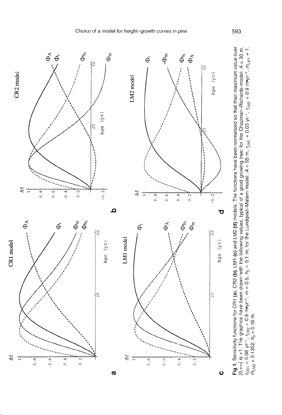
Chapman-Richards
model
It
can
be
seen
on
figure
1a
that,
for
CR1,
the
sensitivity
functions
of
A,
rand
m are
nearly
proportional
on
the
[0,
25]
time
inter-
val.
Figure
1b
shows
that
this
feature
dis-
appears
in
the
second
parametrization,
which
concentrates
the
effects
of
m
in
the
early
ages,
and
those
of
A
in
the
latter
part
of
the
growth
curve.
This
is
likely
to
reduce
e-correlations
between
A
and
r,
and rand
m.
It
should
be
noted
that
fitting
trees
under
20
years
old
will
result
in
imprecise
esti-
mates
for
both
parametrizations:
for
CR1,
precision
will
be
low
for
all
parameters
because
of
e-correlations
between
all
of
them,
while
for
CR2,
imprecision
will
essen-
tially
concern
A,
because
its
sensitivity
func-
tion
is
very
small
and
negative
in
this
time
range.
Lundqvist-Matern
model
The
features
of
the
different
parametriza-
tions
are
essentially
the
same
as
for
the
Chapman-Richards
model.
The
major
dif-
ferences
are
that,
for
the
LM2
model,
the
maximum
of
Φ
m
is
after
50
years
and
the
rise
of
Φ
A
is
slower
than
for
CR2
(fig
1c,d).
The
former
happens
because,
in
the
LM
model,
m
controls
both
the
beginning
of
the
curve
and
its
convergence
rate
to
the
asymptote.
This
is
a
special
property
of
the
LM
model,
and
is
not
shared
by
the
CR
model.
It
is
potentially
misleading
since
a
single
parameter
controls
2
distinct
features
of
the
curve,
between
which
no
evident
bio-
logical link
exists.
It
is
also
likely
to
increase
e-correlation
between
A
and
m,
compared
to
the
CR
model.
The
latter
illustrates
that
although
the
convergence
rate
to
the
asymptote
depends
on
m
(the
curve
converges
to
its
asymptote
in
t
-m
LM1
when
t—>
+∞),
it
is
always
under-
exponential,
while
it
is
exponential
for
the
CR
model.
Both
features
are
intrinsic
prop-
erties of
the
LM
model,
which
do
not
depend
on
the
parametrization.
MATERIAL
AND
METHODS
The
models
were
tested
with
a
data
set
contain-
ing
44
trees
belonging
to
13
good
growing
stands,


%20--%3e%3cdefs%3e%3cstyle%3e%20.st0%20{%20fill:%20%23fff;%20}%20.st1%20{%20fill:%20%237800fa;%20}%20%3c/style%3e%3c/defs%3e%3cpath%20class='st1'%20d='M117.78,12.18H43.11c2.9,3.47,4.65,7.94,4.65,12.82,0,5.6-2.3,10.66-6.01,14.29h76.02l7.22-13.56-7.22-13.56Z'/%3e%3cg%3e%3cpath%20class='st0'%20d='M53.58,26.17h-.59v-1.46h.59v-4.96h2.83c1.78,0,2.67.94,2.67,2.82v5.76c0,1.87-.89,2.81-2.67,2.81h-2.83v-4.96ZM55.36,21.37v3.34h1.1v1.46h-1.1v3.34h1.01c.61,0,.91-.37.91-1.1v-5.93c0-.74-.3-1.1-.91-1.1h-1.01Z'/%3e%3cpath%20class='st0'%20d='M65.99,31.14h-1.8l-.31-2.07h-2.19l-.31,2.07h-1.64l1.82-11.39h2.62l1.82,11.39ZM65.28,18.04c-.25.46-.51.77-.75.94-.21.15-.47.22-.79.22-.26,0-.57-.07-.92-.22l-.38-.15c-.14-.05-.26-.07-.37-.07-.3,0-.53.18-.71.54l-.91-.68c.25-.46.51-.77.75-.94.21-.14.48-.21.79-.21.26,0,.57.07.92.21l.38.15c.14.05.26.07.37.07.3,0,.53-.18.71-.54l.91.68ZM61.91,27.52h1.73l-.87-5.76-.87,5.76Z'/%3e%3cpath%20class='st0'%20d='M74.53,26.89v1.52c0,1.91-.89,2.86-2.67,2.86s-2.67-.95-2.67-2.86v-5.93c0-1.91.89-2.86,2.67-2.86s2.67.95,2.67,2.86v1.11h-1.69v-1.22c0-.75-.31-1.12-.93-1.12s-.93.37-.93,1.12v6.15c0,.74.31,1.11.93,1.11s.93-.37.93-1.11v-1.63h1.69Z'/%3e%3cpath%20class='st0'%20d='M81.4,31.14h-1.8l-.31-2.07h-2.19l-.31,2.07h-1.64l1.82-11.39h2.62l1.82,11.39ZM75.9,19.2l1.52-1.91h1.71l1.51,1.91h-1.61l-.76-.95-.75.95h-1.61ZM77.32,27.52h1.73l-.87-5.76-.87,5.76ZM83.1,15.99l-1.76,1.91h-1.26l1.17-1.91h1.86Z'/%3e%3cpath%20class='st0'%20d='M84.86,19.75c1.78,0,2.67.94,2.67,2.82v1.48c0,1.87-.89,2.81-2.67,2.81h-.85v4.28h-1.79v-11.39h2.64ZM84.01,21.37v3.86h.85c.58,0,.87-.36.87-1.08v-1.71c0-.71-.29-1.07-.87-1.07h-.85Z'/%3e%3cpath%20class='st0'%20d='M93.51,19.75c1.78,0,2.67.94,2.67,2.82v1.48c0,1.87-.89,2.81-2.67,2.81h-.85v4.28h-1.79v-11.39h2.64ZM92.66,21.37v3.86h.85c.58,0,.87-.36.87-1.08v-1.71c0-.71-.29-1.07-.87-1.07h-.85Z'/%3e%3cpath%20class='st0'%20d='M98.8,31.14h-1.79v-11.39h1.79v4.88h2.03v-4.88h1.83v11.39h-1.83v-4.88h-2.03v4.88Z'/%3e%3cpath%20class='st0'%20d='M105.36,24.55h2.46v1.62h-2.46v3.34h3.09v1.63h-4.88v-11.39h4.88v1.63h-3.09v3.18ZM108.17,17.29l-1.76,1.91h-1.26l1.17-1.91h1.86Z'/%3e%3cpath%20class='st0'%20d='M112.2,19.75c1.78,0,2.67.94,2.67,2.82v1.48c0,1.87-.89,2.81-2.67,2.81h-.85v4.28h-1.79v-11.39h2.64ZM111.35,21.37v3.86h.85c.58,0,.87-.36.87-1.08v-1.71c0-.71-.29-1.07-.87-1.07h-.85Z'/%3e%3c/g%3e%3ccircle%20class='st1'%20cx='25'%20cy='25'%20r='20'/%3e%3cpath%20class='st0'%20d='M32.78,19.27c2.92,0,4.43,2.55,5.28,5.33l.71,2.17c.14.38-.33.75-.71.75h-5.61c.19-.33.24-.71.09-1.08l-.75-2.45c-.43-1.32-.99-2.64-1.79-3.77.75-.57,1.65-.94,2.78-.94h0ZM25,18.38c3.25,0,4.9,2.78,5.89,5.89l.76,2.45c.14.42-.33.8-.8.8h-11.69c-.42,0-.94-.38-.8-.8l.75-2.45c.99-3.11,2.64-5.89,5.89-5.89h0ZM25,11.35c1.74,0,3.11,1.37,3.11,3.11s-1.37,3.11-3.11,3.11-3.11-1.41-3.11-3.11,1.41-3.11,3.11-3.11h0ZM17.27,19.27c1.08,0,1.98.38,2.73.94-.8,1.13-1.37,2.45-1.74,3.77l-.8,2.45c-.14.38-.05.75.09,1.08h-5.56c-.42,0-.9-.38-.75-.75l.71-2.17c.9-2.78,2.41-5.33,5.33-5.33h0ZM17.27,12.91c1.51,0,2.78,1.27,2.78,2.83s-1.27,2.83-2.78,2.83-2.83-1.27-2.83-2.83,1.27-2.83,2.83-2.83h0ZM32.78,12.91c1.56,0,2.78,1.27,2.78,2.83s-1.23,2.83-2.78,2.83-2.83-1.27-2.83-2.83,1.27-2.83,2.83-2.83h0ZM27.07,28.56v.09c0,.57-.24,1.08-.61,1.46h0v.05c-.38.33-.9.57-1.46.57s-1.08-.24-1.46-.61h0c-.38-.38-.61-.9-.61-1.46v-.09h1.41v.09c0,.19.05.38.19.47v.05c.09.09.28.19.47.19s.38-.09.47-.19v-.05c.14-.09.24-.28.24-.47t-.05-.09h1.41ZM30.99,28.56v.09c0,1.65-.66,3.16-1.74,4.24-1.08,1.08-2.59,1.79-4.24,1.79s-3.16-.71-4.24-1.79l-.05-.05c-1.04-1.08-1.7-2.55-1.7-4.2v-.09h1.41v.09c0,1.27.47,2.4,1.27,3.25h.05c.85.85,1.98,1.37,3.25,1.37s2.4-.52,3.25-1.37c.85-.8,1.37-1.98,1.37-3.25v-.09h1.37ZM34.99,28.56v.09c0,2.78-1.13,5.28-2.92,7.07-1.79,1.79-4.29,2.92-7.07,2.92s-5.23-1.13-7.07-2.92c-1.79-1.79-2.92-4.29-2.92-7.07v-.09h1.41v.09c0,2.4.94,4.53,2.5,6.08,1.56,1.56,3.72,2.5,6.08,2.5s4.52-.94,6.08-2.5c1.56-1.56,2.5-3.68,2.5-6.08v-.09h1.41Z'/%3e%3c/svg%3e)