Báo cáo toán học: " Robinson-Schensted correspondence for the signed Brauer algebras"

Chia sẻ: Nguyễn Phương Hà Linh Linh | Ngày: | Loại File: PDF | Số trang:26

Thêm vào BST

Báo xấu

67
lượt xem 4
download

Download Vui lòng tải xuống để xem tài liệu đầy đủ

Tuyển tập các báo cáo nghiên cứu khoa học về toán học trên tạp chí toán học quốc tế đề tài: Robinson-Schensted correspondence for the signed Brauer algebras...

Chủ đề:

Bình luận(0) Đăng nhập để gửi bình luận!

Lưu

Nội dung Text: Báo cáo toán học: " Robinson-Schensted correspondence for the signed Brauer algebras"

Robinson-Schensted correspondence for the signed Brauer algebras M. Parvathi and A. Tamilselvi Ramanujan Institute for Advanced Study in Mathematics University of Madras, Chennai-600 005, India sparvathi.riasm@gmail.com,tamilselvi.riasm@gmail.com Submitted: Jan 31, 2007; Accepted: Jul 5, 2007; Published: Jul 19, 2007 Mathematics Subject Classiﬁcations: 05E10, 20C30 Abstract In this paper, we develop the Robinson-Schensted correspondence for the signed Brauer algebra. The Robinson-Schensted correspondence gives the bijection be- tween the set of signed Brauer diagrams d and the pairs of standard bi-domino tableaux of shape λ = (λ1 , λ2 ) with λ1 = (22f ), λ2 ∈ Γf,r where Γf,r = {λ|λ 2(n − 2f ) + |δr | whose 2−core is δr , δr = (r, r − 1, . . . , 1, 0)}, for ﬁxed r ≥ 0 and 0 ≤ f ≤ n . We also give the Robinson-Schensted for the signed Brauer algebra 2 using the vacillating tableau which gives the bijection between the set of signed Brauer diagrams V n and the pairs of d-vacillating tableaux of shape λ ∈ Γ f,r and 0 ≤ f ≤ n . We derive the Knuth relations and the determinantal formula for 2 the signed Brauer algebra by using the Robinson-Schensted correspondence for the standard bi-dominotableau whose core is δ r , r ≥ n − 1. 1 Introduction In [PK], it has been observed that the number of signed Brauer diagrams is the dimension of the regular representation of the signed Brauer algebra, whereas by Artin-Wedderburn structure theorem, the dimension of the regular representation is the sum of the squares of the dimension of the irreducible representations of the signed Brauer algebra which are indexed by partitions λ ∈ Γf,r where Γf,r = {λ|λ 2(n−2f )+|δr | whose 2−core is δr , δr = (r, r − 1, . . . , 1, 0)}, for ﬁxed r ≥ 0 and 0 ≤ f ≤ n . 2 This motivated us to construct an explicit bijection between the set of signed Brauer diagrams V n and the pairs of d-vacillating tableaux of shape λ ∈ Γf,r , for ﬁxed r ≥ 0 and 0 ≤ f ≤ n . We also construct the Robinson-Schensted correspondence for the signed 2 Brauer algebra which gives the bijection between the set of signed Brauer diagrams d and the pairs of standard bi-dominotableaux of shape λ = (λ1 , λ2 ) with λ1 = (22f ), λ2 ∈ Γf,r , for ﬁxed r ≥ 0 and 0 ≤ f ≤ n , which are generalisation of bitableaux introduced by 2 1 the electronic journal of combinatorics 14 (2007), #R49
Enyang [E], while constructing the cell modules for the Birman-Murakami-Wenzl algebras and Brauer algebras with bases indexed by certain bitableau. We also give the method for translating the vacillating tableau to the bi-domino tableau. We also give the Knuth relations and the determinantal formula for the signed Brauer algebra. Since the Brauer algebra is the subalgebra of the signed Brauer algebra, our correspondence restricted to the Brauer algebra is the same as in [DS, HL, Ro1, Ro2, Su]. As a biproduct, we give the Knuth relations and the determinantal formula for the Brauer algebra. 2 Preliminaries We state the basic deﬁnitions and some known results which will be used in this paper. Deﬁnition 2.1. [S] A sequence of non-negative integers λ = (λ1 , λ2 , . . .) is called a partition of n, which is denoted by λ n, if 1. λi ≥ λi+1 , for every i ≥ 1 ∞ 2. λi = n i=1 The λi are called the parts of λ. Deﬁnition 2.2. [S] Suppose λ = (λ1 , λ2 , . . . , λl ) n. The Young diagram of λ is an array of n dots having l left justiﬁed rows with row i containing λi dots for 1 ≤ i ≤ l. Example 2.3. ∗ ∗ · · · ∗ λ1 nodes ∗ ∗ · ·∗ λ2 nodes · · · [λ] := · · · · · · ∗ ∗ ··· ∗ λr nodes Deﬁnition 2.4. [JK] Let α be a partition of n, denoted by α n. Then the (i, j )-hook of α α, denoted by Hi,j which is deﬁned to be a Γ-shaped subset of diagram α which consists of the (i, j )-node called the corner of the hook and all the nodes to the right of it in the same row together with all the nodes lower down and in the same column as the corner. α The number hij of nodes of Hij i.e., hij = αi − j + αj − i + 1 α where αj = number of nodes in the j th column of α, is called the length of Hi,j , where α = [α1 , · · · αk ]. A hook of length q is called a q -hook. Then H [α] = (hij ) is called the hook graph of α. 2 the electronic journal of combinatorics 14 (2007), #R49
Deﬁnition 2.5. [R] We shall call the (i, j ) node of λ, an r -node if and only if j − i ≡ r (mod2). Deﬁnition 2.6. [R] A node (i, j ) is said to be a (2, r ) node if hij = 2m and the residue of node (i, λi ) in λ is r . i.e. λi − i ≡ r (mod2). Deﬁnition 2.7. [R]. If we delete all the elements in the hook graph H [λ] not divisible by 2, then the remaining elements, hij = hr (2), (r = 0, 1) ij can be divided into disjoint sets whose (2, r ) nodes constitute the diagram [λ]r , (r = 0, 1) 2 with hook graph (hr ). The λ is written as (λ1 , λ2 ) where the nodes in λ1 correspond to ij (2, 0) nodes and the nodes in λ2 correspond to (2, 1) nodes. Deﬁnition 2.8. [JK] Let λ n. An (i, j )-node of λ is said to be a rim node if there does not exist any (i + 1, j + 1)-node of λ. Deﬁnition 2.9. [JK] A 2-hook comprising of rim nodes is called a rim 2-hook. Deﬁnition 2.10. [JK] A Young diagram λ which does not contain any 2-hook is called 2-core. Deﬁnition 2.11. [JK] Each 2 × 1 and 1 × 2 rectangular boxes consisting of two nodes is called as a domino. Lemma 2.12. [PST] Let ρ ∈ Γ0,r , for ﬁxed r ≥ 0. Then ρ can be associated to a pair of partitions as in Deﬁnition 2.7, but when associated to a pair of partitions through the map η we have, every domino in row i of ρ corresponds to a node of λi and every domino in column j of ρ corresponds to a node of µj . Proposition 2.13. [PST] If x ∈ Sn , the hyperoctahedral group of type Bn then P (x−1 ) = Q(x) and Q(x−1 ) = P (x) where P (x), Q(x), P (x−1 ), Q(x−1 ) are the standard tableaux of shape λ ∈ Γ0,r , for ﬁxed r ≥ n − 1. Proposition 2.14. [BI, PST] If x, y ∈ Sn , the hyperoctahedral group of type Bn then K x ∼ y ⇐⇒ P (x) = P (y ) where P (x), P (y ) are the standard tableaux of shape λ ∈ Γ0,r , for ﬁxed r ≥ n − 1. Deﬁnition 2.15. [PST] Let ρ ∈ Γ0,r , r ≥ 0. We deﬁne a map η : ρ → (ρ(1) , ρ(2) ), λ l, µ m, l + m = n such that if r is even 1 (1) (ρi − (n − i)) if ρi > n − i ρi = 2 1 (2) (2) 1 where ρj = (ρj − (n − j)) if ρj > n − j ρi = 2 j µj ≥i 3 the electronic journal of combinatorics 14 (2007), #R49
if r is odd 1 (1) (ρi − (n − i) + 1) if ρi > n − i − 1 ρi = 2 1 (2) (2) 1 where ρj = (ρj − (n − j) + 1) if ρj > n − j − 1 ρi = 2 j µj ≥i 1 n then f λ = n! Proposition 2.16. [S] If λ = (λ1 , λ2 , . . . , λl ) . (λi − i + j )! l×l 2.1 The Brauer algebras Deﬁnition 2.17. [Br] A Brauer graph is a graph on 2n vertices with n edges, vertices being arranged in two rows each row consisting of n vertices and every vertex is the vertex of only one edge. 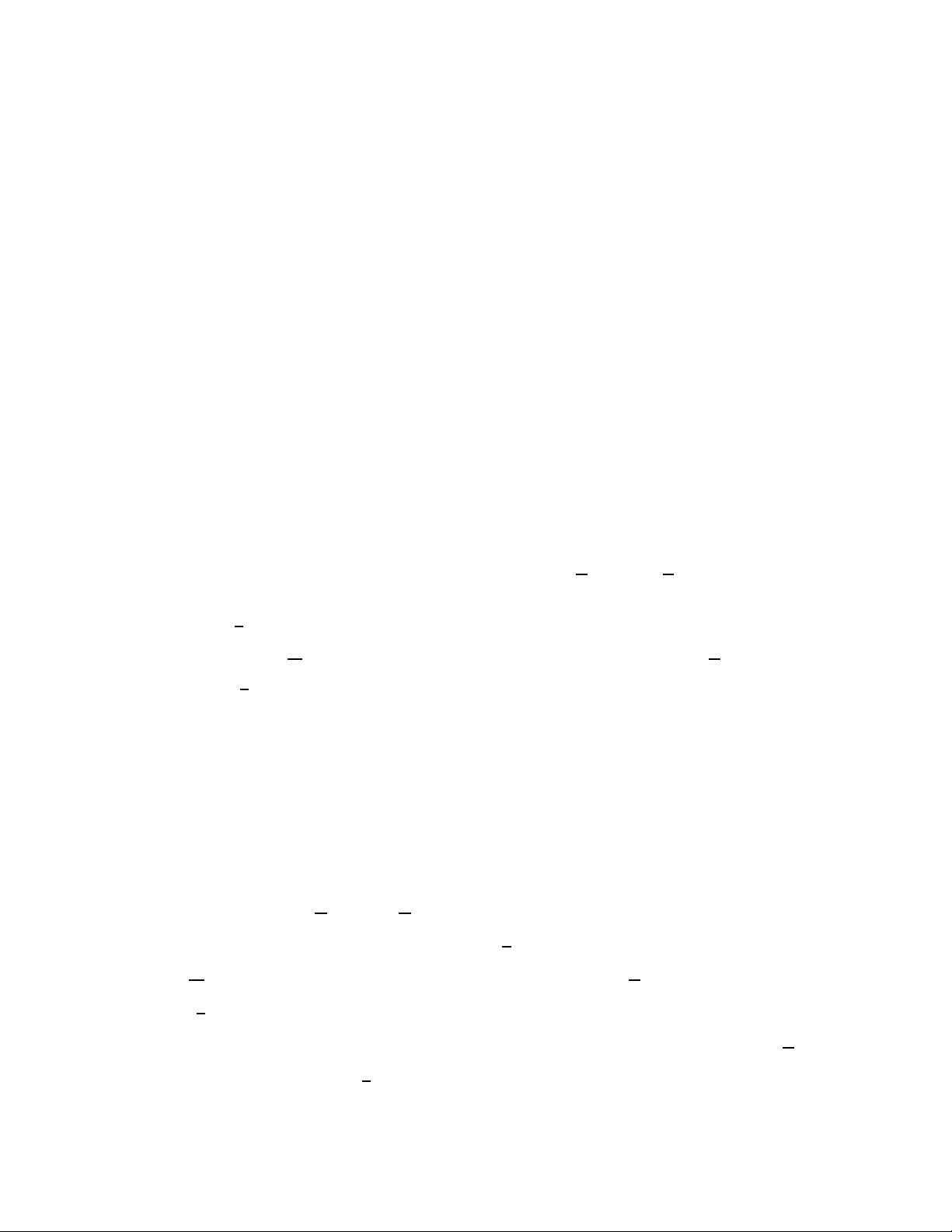Deﬁnition 2.18. [Br] Let Vn denote the set of Brauer graphs on 2n vertices. Let d, d ∈ Vn . The multiplication of two graphs is deﬁned as follows: 1. Place d above d . 2. join the ith lower vertex of d with ith upper vertex of d 3. Let c be the resulting graph obtain without loops. Then ab = xr c, where r is the number of loops, and x is a variable. For example, q q q q q q d= q q q q q q q q q q q q d= q q q q q q q q q q q q dd = q q q q q q q q q q q q q q q q q q =c q q q q q q The Brauer algebra Dn (x), where x is an indeterminate, is the span of the diagrams on n dots where the multiplication for the basis elements deﬁned above. The dimension of Dn (x) is (2n)!! = (2n − 1)(2n − 3) . . . 3.1. 4 the electronic journal of combinatorics 14 (2007), #R49
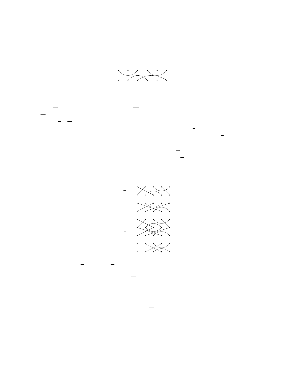
2.2 The signed Brauer algebras Deﬁnition 2.19. [PK] A signed diagram is a Brauer graph in which every edge is labeled by a + or a − sign. 1 2 3 4 5 6 R 1 2 3 4 5 6 Deﬁnition 2.20. [PK] Let Vn denote the set of all signed Brauer graphs on 2n vertices with n signed edges. Let Dn (x) denote the linear span of Vn where x is an indeterminate. The dimension of D n (x) is 2n (2n)!! = 2n (2n − 1)(2n − 3) . . . 3.1. 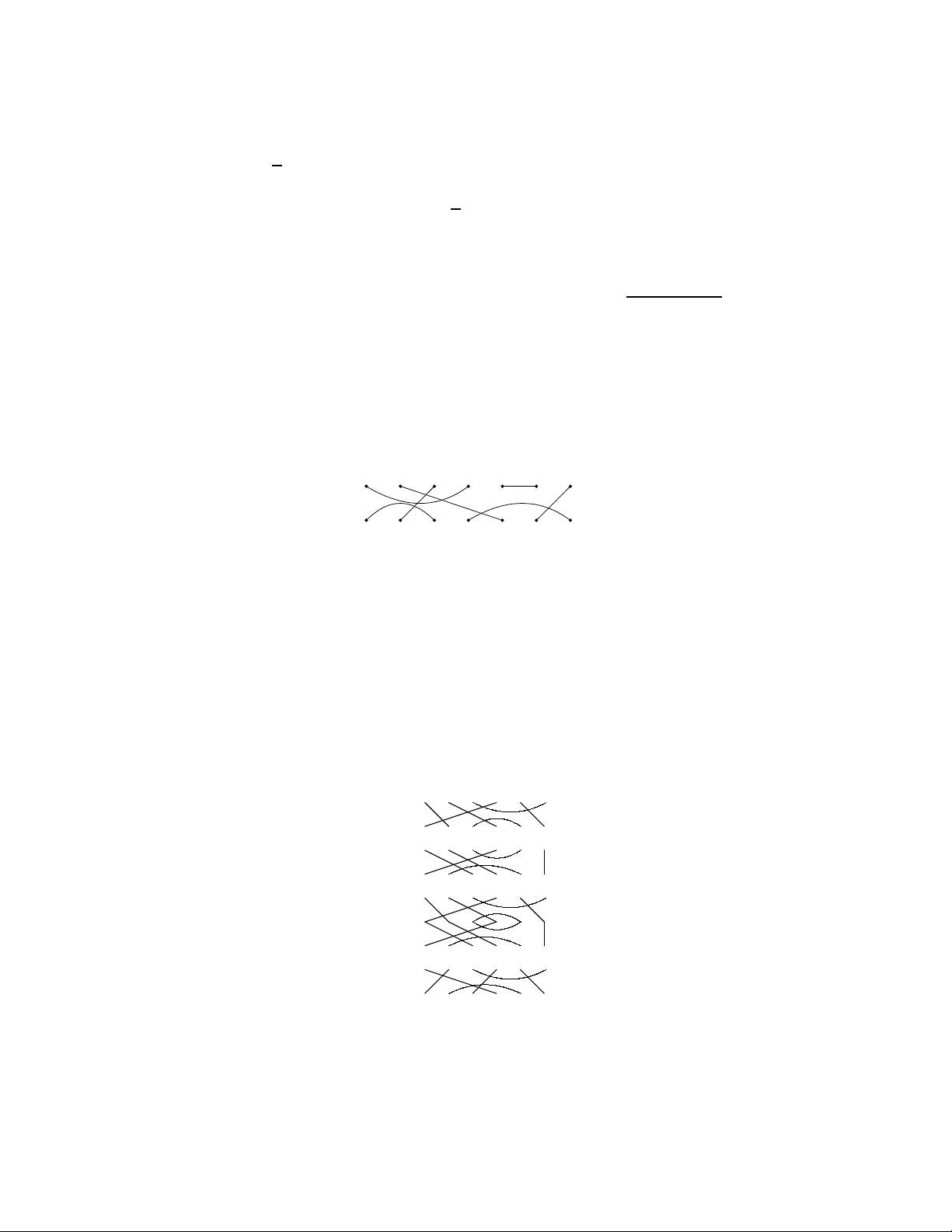Let a, b ∈ V n . Since a, b are Brauer graphs, ab = xd c, the only thing we have to do is to assign a direction for every edge. An edge α in the product ab will be labeled as a + or a − sign according as the number of negative edges involved from a and b to make α is even or odd. A loop β is said to be a positive or a negative loop in ab according as the number of negative edges involved in the loop β is even or odd. Then ab = x2d1 +d2 , where d1 is the number of positive loops and d2 is the number of negative loops. Then D n (x) is a ﬁnite dimensional algebra. For example, Y a= R 1 * b= R Y *R1 ba = R * =x R [n] 2 Γf,r , where Γf,r = {λ|λ 2(n − 2f ) + |δr | whose 2-core is δr , δr = Let Γn,r = f =0 (r, r − 1, . . . , 1, 0)} for ﬁxed r ≥ 0. Let B be the Bratteli diagram whose vertices on the k th ﬂoor are members of Γn,r . Note that 0th ﬂoor contains precisely the core δr . The ith vertex on the k th ﬂoor and j th vertex on the (k − 1)th ﬂoor are joined whenever the latter is obtained from the former by removing a rim 2-hook. Deﬁnition 2.21. [PK] An up-down path p in B is deﬁned as the sequence of partitions in Γn,r starting from the 0th ﬂoor to the 1nth ﬂoor. i.e. it can be considered as p = [δr = λ0 , λ1 , . . . , λn ] where λi is obtained from λi−1 either by adding or removing of only one rim 2-hook. 5 the electronic journal of combinatorics 14 (2007), #R49
Let |Ωn | denote the number of up-down paths ending at the nth ﬂoor. |Ωn,λ | denotes the number of up-down paths ending at λ in the nth ﬂoor. The paths belong to Ωn,λ are called the d-vacillating tableau of shape λ, λ ∈ Γn,r . 3 The Robinson-Schensted correspondence for the signed Brauer algebras 3.1 The Robinson-Schensted correspondence using bi-domino tableau In this section, we deﬁne a Robinson-Schensted algorithm for the signed Brauer algebra which gives the correspondence between the signed Brauer diagram d and the pairs of standard bi-dominotableaux of shape λ = (λ1 , λ2 ) with λ1 = (22f ), λ2 ∈ Γf,r , for ﬁxed r ≥ 0 and 0 ≤ f ≤ n .2 Deﬁnition 3.1. A domino in which all the nodes are ﬁlled with same number from the set A = {1, 2, · · · n} is deﬁned as a tablet. Deﬁnition 3.2. A bipartition ν of 2n will be an ordered pair of partitions (ν (1) , ν (2) ) where ν (1) = (22f ) and ν (2) ∈ Γf,r , for ﬁxed r ≥ 0. Deﬁnition 3.3. A standard horizontal block is deﬁned as the block consisting of two d(1) d(1) horizontal tablets d(1) , d(2) one above the other such that d(1) < d(2) . i.e. . d(2) d(2) We call d(1) as the ﬁrst tablet of the horizontal block and d(2) as the second tablet of the horizontal block. We call horizontal block as positive block. Deﬁnition 3.4. A standard vertical block is deﬁned as the block consisting of two vertical d(1) d(2) tablets d(1) , d(2) adjacent to each other such that d(1) < d(2) . i.e. (1) . We call d(1) d(2) d as the ﬁrst tablet of the vertical block and d(2) as the second tablet of the vertical block. We call vertical block as negative block. Deﬁnition 3.5. A block tableau is a tableau consisting either of the horizontal block or the vertical block. Deﬁnition 3.6. A column standard block tableau is a block tableau if the head nodes of the ﬁrst tablets of each block are increasing read from top to bottom. Deﬁnition 3.7. A standard tableau is a tableau consisting of tablets such that the head nodes of the tablets are increasing along the rows and increasing along the columns. Deﬁnition 3.8. Let ν (1) , ν (2) be as in Deﬁnition 3.2. A ν -bi-dominotableau t is standard if t(1) is the column standard block tableau and t(2) is the standard tableau. The collection of standard ν -bi-dominotableaux will be denoted by Std(ν ). 6 the electronic journal of combinatorics 14 (2007), #R49
Deﬁnition 3.9. Given a signed Brauer diagram d ∈ V n , we may associate a triple [d1 , d2 , w ] such that d1 = { (i, d1 (i), c(d1 (i)))| the edge joining the vertices i and d1 (i) in the ﬁrst row with sign c(d1 (i))} = {(i1 , d1 (i1 ), c(d1 (i1 ))), (i2 , d1 (i2 ), c(d1 (i2 ))), . . . , (if , d1 (if ), c(d1 (if )))} d2 = { (j, d2 (j ), c(d2 (j )))| the edge joining the vertices j and d2 (j ) in the second row with sign c(d2 (j ))} = {(i1 , d2 (i1 ), c(d2 (i1 ))), (i2 , d2 (i2 ), c(d2 (i2 ))), . . . , (if , d2 (if ), c(d2 (if )))} w = { (k, w (k ), c(w (k )))| the edge joining the vertex k in the ﬁrst row and w (k ) in the second row with sign c(w (k ))} = {(i1 , w (i1 ), c(w (i1 ))), (i2 , w (i2 ), c(w (i2 ))), . . . , (in−2f , w (in−2f ), c(w (in−2f )))} such that i1 < i2 < . . . < in−2f where f is the number of horizontal edges in a row of d and n − 2f is the number of vertical edges in d and c(x) = the sign of the edge joining between x and its preimage, c(x) ∈ {±1}. R−S Theorem 3.10. The map d ←→ [(P1 (d), P2 (d)), (Q1 (d), Q2 (d))] provides a bijection be- tween the set of signed Brauer diagrams d and the pairs of standard λ-bi-dominotableaux. Proof. We ﬁrst describe the map that, given a diagram d ∈ V n , produces a pair of bi- R−S dominotableaux. d ←→ [(P1 (d), P2 (d)), (Q1 (d), Q2 (d))] We construct a sequence of tableaux f 0 1 ∅ = P 1 , P1 , . . . , P1 Q 0 , Q1 , . . . , Qf ∅ = 1 1 1 n−2f 0 1 ∅ = P 2 , P2 , . . . , P2 Q0 , Q1 , . . . , Q2 −2f n ∅ = 2 2 where f is the number of horizontal edges, the edges joining the vertices (x1 , x2 ) with the sign c are inserted into P1 (d), P2 (d), Q1 (d) and placed in Q2 (d) so that shP1 =shQk , for k 1 all k and shP2 =shQj , for all j . j 2 Begin with the tableau P1 = Q0 = ∅ and P2 = Q0 = t0 , where t0 is the tableau of 0 0 1 2 shape δr , for ﬁxed r ≥ 0 with entries 0’s. Then recursively deﬁne the standard tableau by the following. of (l, m) in P1 −1 . k k If (l , m ) ∈ d2 then P1 = insertion of (l, m) in Q1 −1 . If (l, m) ∈ d1 then Qk = k insertion 1 of m in P2 −1 and place l in Q2 −1 where the k k k If (l, m ) ∈ w then P2 = insertion terminates in P2 −1 when m is inserted. k insertion The operations of insertion and placement will now be described. 7 the electronic journal of combinatorics 14 (2007), #R49
First we give the insertion on P1 (d). Let (ik , d2 (ik ), c(d2 (ik ))) ∈ d2 and ik , d2 (ik ) be the elements not in P1 (d). To insert ik , d2 (ik ) with sign c(d2 (ik )) into P1 (d), we proceed as follows. ik ik If c(d2 (ik )) = 1 then the positive block i.e. is to be inserted into P1 (d) d2 (ik ) d2 (ik ) along the cells (i, j ), (i, j + 1), (i + 1, j ), (i + 1, j + 1). i d2 (ik ) If c(d2 (ik )) = −1 then the negative block i.e. βx = k is to be inserted into ik d2 (ik ) P1 (d) along the cells (i, j ), (i + 1, j ), (i, j + 1), (i + 1, j + 1). Now place the block containing ik , d2 (ik ) below the block containing ik−1 , d2 (ik−1 ). Insertion on Q1 (d) is the same as in P1 (d). Insertion on P2 (d) is the same as in the case of hyperoctahedral group. We give it here for the sake of completion. Algorithm BDT Let w (x) be the element not in P2 (d). To insert w (x) in P2 (d), we proceed as follows. If c(w (x)) = 1 then the horizontal tablet αw(x) = w (x) w (x) is to be inserted into P2 (d) along the cells (i, j ) and (i, j + 1). The (i, j + 1)th cell of αx is called the head node of αw(x) and the (i, j )th cell of αw(x) is called the tail node of αw(x) . w (x) If c(w (x)) = −1 then the vertical tablet βw(x) = is to be inserted into P2 (d) w (x) along the cells (i, j ) and (i + 1, j ). The (i, j )th cell of βw(x) is called the head node of βw(x) and the (i + 1, j )th cell of βw(x) is called the tail node of βw(x) . If c(w (x)) = 1 then, A Set row i := 1, head node of αw(x) := w (x) and tail node of αw(x) := w (x). B If head node of αw(x) is less than some element of row i then Let y1 be the smallest element of row i greater than y1 y2 i w (x) such that the north west most corner of the j domino containing y1 is in the cell (i, j ) and y2 be the element in the cell (i, j + 1). 2 cases arise, y1 y1 i (BI) tablet containing y1 is horizontal i.e., αy1 . j (y1 = y2 ) y1 y2 i (BII) tablet containing y1 is vertical i.e., βy1 . y1 (y1 = y2 ) j BI If the tablet containing y1 is αy1 (head node of αy1 is in the cell (i, j + 1) and the tail node of αy1 is in the cell (i, j ) ) i.e. y1 = y2 then, replace tablet αy1 by tablet αw(x) . Set tablet αw(x) := tablet αy1 , Row i := i + 1 and go to B. 8 the electronic journal of combinatorics 14 (2007), #R49
BII If the tablet containing y1 is βy1 . (i.e. head node of βy1 is in the cell (i, j ) and the tail node of βy1 is in the cell (i + 1, j ) ) i.e. y1 = y2 then y1 y2 i Let w1 be the element in the cell (i + 1, j + 1). y1 w1 j 2 cases arise y1 y2 i BIIa w1 = y2 y1 y2 j y1 y2 i BIIb w1 = y2 y1 w1 j BIIa If w1 = y2 then replace w1 by y1 and set tablet βw(x) = y2 and column j := j +2 and go to B . (B is the case as in B by replacing row by column, column by row, positive tablet by negative tablet and negative tablet by positive tablet.) BIIb If w1 = y2 then let w2 be the element in the cell (i + 1, j + 2). Replace w1 and w2 by y1 and y2 respectively, and set y1 := w1 , y2 := w2 , row i := i +1. If x1 = x2 then set row i := i + 1 and go to B else go to BII. C Now head node of αw(x) is greater than every element of row i so place the tablet αw(x) at the end of the row i and stop. If c(w (x)) = −1 then, replace row by column, column by row, positive tablet by negative tablet and negative tablet by positive tablet in the positive case. The placement of the tablet of an element in a tableau is even easier than the insertion. Suppose that Q2 (d) is a partial tableau of shape µ and if k is greater than every element of Q2 (d), then place the tablet of k in Q2 (d) along the cells where the insertion in P2 (d) terminates. R−S To prove [(P1 (d), P2 (d)), (Q1 (d), Q2 (d))] −→ d . We merely reverse the preceding algorithm step by step. We begin by deﬁning [(P1 , P2 −2f ), (Qf , Q2 −2f )] = [(P1 (d), P2 (d)), (Q1 (d), Q2 (d))] f n n 1 where f is the number of horizontal edges in a row of d and n − 2f is the number of vertical edges in d. Reverse Algorithm BDT. Assuming that P2 and Qk has been constructed we will ﬁnd k 2 the pair (xk , w (xk ), c(w (xk ))) and [(P1 −1 , P2 −1 ), (Q1 −1 , Q2 −1 )]. k k k k xk Find the cells containing the tablet of xk in Q2 . 2 cases arise, † The cells containing tablet of xk in Qxk are (i, j − 1) and (i, j ) 2 ‡ The cells containing tablet of xk in Qxk are (i − 1, j ) and (i, j ) 2 9 the electronic journal of combinatorics 14 (2007), #R49
case † If the cells containing tablet of xk in Qxk are (i, j − 1) and (i, j ), then since this 2 is the largest element whose tablet appears in Qxk , P2 −1 , P2 must have been the i,j i,j 2 xk last element to be placed in the construction of P2 . We can now use the following procedure to delete P2 −1 , P2 from P2 (d). For i,j i,j convenience, we assume the existence of an empty zeroth row above the ﬁrst row of x x P2 k and empty zeroth column to the left of the ﬁrst column of P2 k . Set x1 := P2 −1 , x2 := P2 and erase P2 −1 , P2 . i,j i,j i,j i,j 2 cases arise, (A) x1 = x2 (B) x1 = x2 case A If x1 = x2 then case AI Set head node of αx := x2 and tail node of αx := x1 and Row x i := (i − 1)th row of P2 k . x case AII If Row i is not the zeroth row of P2 k then Let y be the largest element of Row i smaller than w (x) which is in the cell (i, l) (2 cases arise, (AIIa) the tablet containing y is αy (AIIb) the tablet containing y is βy ) case AIIa If the tablet containing y is αy then replace tablet αy by tablet αx . Set tablet αx := tablet αy , Row i := i−1 and goto AII case AIIb If the tablet containing y is βy then Let z be the element in the cell (i, l − 1) and replace tail node of βy and z by tablet αx . Set x1 := z and x2 := tail node of βy and go to B. case AIII Now the tablet αx has been removed from the ﬁrst row, so set w (xk ) := x and c(w (xk )) = 1. case B If x1 = x2 then 2 cases arise, (B1) the tablet containing x1 is βx1 (B2) the tablet containing x1 is αx1 case B1 If the tablet containing x1 is βx1 then replace head node of βx1 by tail node of βx2 . Set tablet βw(x) := tablet βx1 and Column j := j − 2 and go to A I I. (A I I is the case as in AII by replacing row by column, column by row, positive tablet by negative tablet and negative tablet by positive tablet.) case B2 If the tablet containing x1 is αx1 then replace the elements in the cell (i − 1, j − 2) and (i − 1, j − 1) by head node of αx1 and tail node of βx2 respectively. Set x1 := the element in the cell 10 the electronic journal of combinatorics 14 (2007), #R49
(i − 1, j − 2), x2 := the element in the cell (i − 1, j − 1) and if x1 = x2 then Row i := i − 1 and go to A else Column j = j − 1 and go to B. case ‡ follows as in case † by replacing row by column, column by row, positive tablet by negative tablet and negative tablet by positive tablet. It is easy to see that P2 k −1 is P2 k after the deletion process complete and Qxk −1 is Qxk x x 2 2 with the tablet of xk erased. Continuing in this way, we recover all the elements of w in reverse order. We are yet to ﬁnd the elements in d1 , d2 . We may recover the elements of d2 such that the pair (xk , d2 (xk ), c(d2 (xk ))) is the block in the cells ((2k − 1, 1), (2k − 1, 2), (2k, 1), (2k, 2)) of P1 (d), for every k and the c(d2 (xk )) = 1 (c(d2 (xk )) = −1) if the block is positive block (negative block). Similarly, we may recover the elements of d1 such that the pair (xk , d1 (xk ), c(d1 (xk ))) is the element in the cells ((2k − 1, 1), (2k − 1, 2), (2k, 1), (2k, 2)) of Q1 (d), for every k and the c(d1 (xk )) = 1 (c(d1 (xk )) = −1) if the block is positive block (negative block). Thus we recover the triple d1 , d2 , w from the pair of bi-dominotableaux [(P1 (d), P2 (d)), (Q1 (d), Q2 (d))]. R−S Hence [(P1 (d), P2 (d)), (Q1 (d), Q2 (d))] −→ d which completes the proof. Example 3.11. Let 1 2 3 4 5 6 7 d= R 1 2 3 4 5 6 7 d1 = {(1, 3, −1), (4, 6, 1)} d2 = {(2 , 4 , 1), (3 , 6 , −1)} w = {(2, 1 , −1), (5, 7 , 1), (7, 5 , 1)} 2 2 2 2 4 4 0 1 2 P1 = ∅ P1 = P1 = 4 4 3 6 3 6 1 3 1 3 13 Q0 = ∅ Q1 = Q2 = 1 1 1 13 4 4 6 6 For the core δr , r = 0, we have 1 15 5 177 0 1 2 3 P2 = ∅ P2 = P2 = P2 = 1 17 7 1 11 the electronic journal of combinatorics 14 (2007), #R49
2 25 5 2 55 Q0 = ∅ Q1 = Q2 = Q3 = 2 2 2 2 2 27 7 2 Thus    2 2 1 3  4 3  1 4 155 2 55 R−S d ←→   ,  , ,  3 4  4 177 2 77 6 3 6 6 6 For the core δr , r = (2, 1), the above diagram gives 0 0 00 77 0 055 00 0 0 0 77 0 1 2 3 P2 = P2 = P2 = P2 = 0 1 1 1 1 1 1 0 0 00 55 00 55 00 0 0 07 7 Q0 = Q1 = Q2 = Q3 = 2 2 2 2 0 2 2 2 2 2 2 Thus    2 2 1 3 0 055 0 05 5  4  0  1 3  4 77 0 77 R−S d ←→    , , ,  3 4  1  4 2 6 1 2 3 6 6 6 Remark 3.12. If d ∈ V n has no horizontal edges (d1 = d2 = ∅) then d is an element in the hyperoctahedral group. Hence P1 (d) = ∅, Q1 (d) = ∅, P2 (d) = P, Q2 (d) = Q where P1 (d), Q1 (d) are the column standard block tableau and P2 (d), Q2 (d) are the stan- dard tableau constructed by the above insertion and P, Q are the tableaux of shape λ ∈ Γ0,r , for ﬁxed r ≥ 0 constructed by the Robinson-Schensted correspondence for the hyperoctahedral group of type Bn . R−S Corollary 3.13. The map d ←→ [(P1 (d), P2 (d)), (Q1 (d), Q2 (d))] provides a bijection between the set of Brauer diagrams d and the pairs of standard bitableaux of shape λ = (λ1 , λ2 ) with λ1 = (2f ), λ2 ∈ Γf where Γf = {λ|λ n − 2f } and 0 ≤ f ≤ [ n ]. 2 12 the electronic journal of combinatorics 14 (2007), #R49
Proof. Each signed Brauer diagram is a Brauer diagram if and only if each edge is labelled by a positive sign and the proof follows by replacing each positive tablet x by the node x in Theorem 3.10. Deﬁnition 3.14. The ﬂip of any signed Brauer diagram d is the diagram of d reﬂected over its horizontal axis, which is denoted by ﬂip(d). Proposition 3.15. Let d ∈ V n . If d −→ [(P1 (d), P2 (d)), (Q1 (d), Q2 (d))]. Then ﬂip(d) −→ [(Q1 (d), Q2 (d)), (P1 (d), P2 (d))] where P1 (d), Q1 (d) are the column standard block tableaux and P2 (d), Q2 (d) are the standard tableaux constructed by the above insertion. Proof. Suppose d ∈ V n , then we can recover the triple [d1 , d2 , w ] by the Deﬁnition 3.9. By the deﬁnition ﬂip(d) has the triple [d2 , d1 , w −1 ]. Hence the proof follows by Proposition 2.13. 3.2 The Robinson-Schensted correspondence using vacillating tableau In this section, we follow the Robinson-Schensted correspondence using vacillating tableau for the Partition algebras in [HL], to construct the Robinson-Schensted correspondence for the signed Brauer algebras. Let us denote by Tn (λ) the set of d-vacillating tableaux of shape λ and length n + 1. Thus |Ωn,λ | = |Tn (λ)|. To give a combinatorial proof of n |Ωn,λ |2 2n (2n)!! = for ﬁxed r ≥ 0 and 0 ≤ f ≤ 2 e λ∈Γf,r we ﬁnd a bijection of the form n V n ←→ Tn (λ) × Tn (λ) for ﬁxed r ≥ 0 and 0 ≤ f ≤ 2 λ∈Γf,r ,r ≥0 by constructing a function that takes a signed Brauer diagram d ∈ V n and produces a pair (Pλ , Qλ ) of d-vacillating tableaux. We will draw diagrams d ∈ V n using a standard representation as a single row repre- sentation with 2n vertices labeled 1, 2, . . . , 2n, where we relabel vertex j with the label (2n − j + 1). We draw the edges of the standard representation of d ∈ V n in a speciﬁc way such that: Connect the vertices i and j for i ≤ j if and only if i and j are related in d. In this way, connect each vertex. We label each positive edge of the diagram d with (2n − m + 1) where m is the right vertex and each negative edge of the diagram d with −(2n − m + 1). 13 the electronic journal of combinatorics 14 (2007), #R49
Deﬁnition 3.16. The insertion sequence of a diagram d ∈ V n to be the sequence I (d,n) = (d,n) (Ij ) indexed by j in the sequence 1, 2, . . . , 2n, where  a, if vertex j is left endpoint of positive edge a;  (d,n) −a, if vertex j is left endpoint of negative edge a; Ij =  (a, ∅), if vertex j is right endpoint of either a positive or a negative edge a. ··· j 1 2 2n Thus the insertion sequence is (d,n) ··· Ij x1 x2 x2n Proposition 3.17. d ∈ V n is completely determined by its insertion sequence. Proof. The proof is the same as in [HL], we give it here for the sake of completion. Since the insertion sequence of a diagram d completely determines the edges, the proof follows. d (d,n) (d,n) ←− T (j −1) means the domino containing Ij is deleted from T (j −1) and Note. Ij (d,n) R−S (d,n) −→ T (j −1) means the domino containing Ij is to be inserted in T (j −1) using Ij algorithm BDT in theorem 3.10. (d,n) For d ∈ V n with insertion sequence I (d,n) = (Ij ), we will produce a pair (Pλ , Qλ ) of d-vacillating tableaux. Let T (0) be the tableau of shape δr with entries 0’s. Then recursively deﬁne standard tableau T (j +1) by (d,n) R−S (d,n) Ij +1 −→ T (j ) if Ij +1 = xk (j +1) T = d (d,n) (d,n) Ij +1 ←− T (j ) if Ij +1 = (xk , ∅). Let λ(i) be the shape of T (i) . Deﬁne Qλ = (δr , λ(1) , . . . , λ(n) ) ∈ Tn (λ) (3.1) (2n) (n) ) ∈ Tn (λ) Pλ = (λ ,...,λ (3.2) In this way, we associate a pair of d-vacillating tableaux (Pλ , Qλ ) to d ∈ V n which we R−S denote by d −→ (Pλ , Qλ ). Vn R−S Theorem 3.18. The map d ←→ (Pλ , Qλ ) provides a bijection between the set of signed Vn Brauer diagrams V n and the pairs of d-vacillating tableaux of shape λ ∈ Γf,r , for ﬁxed r ≥ 0 and 0 ≤ f ≤ n . i.e. 2 V n ←→ Tn (λ) × Tn (λ) λ∈Γf,r ,r ≥0 14 the electronic journal of combinatorics 14 (2007), #R49
Proof. The proof is same as in [HL], we give it here for the sake of completion. We prove R−S the theorem by constructing the inverse of d −→ (Pλ , Qλ ). First we use Qλ followed by Vn Pλ in reverse order to construct the sequence λ , λ(2) , . . . , λ(2n) . We initialize T (2n) = ∅. (1) (d,n) d,n R−S We now show how to construct T (i) and Ii+1 so that T (i+1) = Ii(+1 ) −→ T (i) . If λ(i+1) /λ(i) is a tablet a, and we use reverse algorithm BDT on the value in the tablet a to (d,n) d,n R−S produce T (i) and Ii+1 such that T (i+1) = Ii(+1 ) −→ T (i) . Since we remove the value in position a by using reverse Robinson-Schensted algorithm, we know that T (i) has shape λ(i) . (d,n) d We then show how to construct T (i) and Ii+1 so that T (i+1) = Ii(+1 ) ←− T (i) . d,n If λ(i) /λ(i+1) is a tablet a. Let T (i) be the tableau of shape λ(i) with the same entries (d,n) as T (i+1) and having the entry 2n − i in tablet a. Let Ii+1 = 2n − i. At any given step i, 2n − i is the largest domino added to the tableau thus far, so T (i) is standard. (d,n) d Furthermore, T (i+1) = Ii(+1 ) ←− T (i) , since Ii+1 = 2n − i is already in the rim hook d,n and thus simply delete it. (d,n) (d,n) (d,n) This iterative process will produce I2n , I2n−1 , . . . , I1 which completely determines R−S d. By the way we have constructed d, we have d ←→ (Pλ , Qλ ). Vn Example 3.19. Let d be the diagram as in Example 3.11. Then the single row represen- tation of d is −1 −3 7 5 12 9 2 j R R 1 2 3 4 5 6 7 8 9 10 11 12 13 14 and the insertion sequence is j 1 2 3 45 6 7 8 (d,n) 12 −1 (12, ∅) 9 7 (9, ∅) 5 (7, ∅) Ij j 9 10 11 12 13 14 (d,n) −3 (5, ∅) 2 (−3, ∅) (2, ∅) (−1, ∅) Ij For the core δr , r = 0, we have (d,n) (d,n) T (j ) T (j ) j Ij j Ij d ∅ 14 (−1, ∅) ←− ∅ 0 15 the electronic journal of combinatorics 14 (2007), #R49
(d,n) (d,n) T (j ) T (j ) j Ij j Ij 1 d R−S −→ 13 (2, ∅) ←− 12 12 1 12 1 1 12 12 2 d R−S 2 −1 −→ 12 (−3, ∅) ←− 1 12 1 12 2 1 1 d R−S 3 (12, ∅) ←− −→ 11 2 1 3 3 1 199 1 d R−S −→ 10 (5, ∅) ←− 49 1 3 3 15 5 177 1 R−S R−S −→ −3 −→ 57 9 199 3 3 177 15 5 d d 6 (9, ∅) ←− (7, ∅) ←− 8 1 1 155 15 5 R−S R−S −→ −→ 75 7 5 177 17 7 R−S Hence d −→ (Pλ , Qλ ) where Vn     Pλ =  ∅,  , , , , , ,   ∅, Qλ = , , , , , , Remark 3.20. 1. Replace the domino as a node in the above procedure, we get the Robinson-Schensted correspondence for the Brauer algebra, which gives the same vacillating tableau as in [DS, HL, Ro1, Ro2, Su]. 16 the electronic journal of combinatorics 14 (2007), #R49
2. We can pass from vacillating tableau to the bi-domino tableau by the following proce- dure: Let (Pλ , Qλ ) be the vacillating tableau obtained using the Robinson-Schensted cor- respondence for the vacillating tableau. If a positive (negative) domino is added at the ith step in Pλ then put i in that domino. If a domino is removed at the ith step in a vacillating tableau Pλ then perform reverse algorithm BDT in Theorem 3.10. A number j with positive or negative sign is uninserted. Now add the positive or negative domino block in P1 (d). The ﬁnal tableau obtained using the above procedure is P1 (d). Similarly, construct Q1 (d) and Q2 (d) using Qλ . 4 Applications of Robinson-Schensted correspondence for the signed Brauer algebra using bidomino tableau 4.1 The Knuth relations In this section, we derive the Knuth relations for the signed Brauer algebra by using the Robinson-Schensted correspondence for the standard bi-dominotableau whose 2-core is δr , r ≥ n − 1. Deﬁnition 4.1. A generalized signed permutation is a two-line array of integers i1 i2 ... in x= ε x 1 x1 ε x 2 x2 . . . ε x n xn where εxi ∈ {±1}, ∀i whose column are in lexicographic order, with the top entry taking precedence and xl = xm , ∀ l, m. The set of all generalized signed permutations is denoted by GSP (n) Proposition 4.2. If x ∈ GSP (n) then P (x−1 ) = Q(x) and Q(x−1 ) = P (x) where P (x), P (x−1 ), Q(x), Q(x−1 ) be the standard tableaux of shape λ ∈ Γ0,r , for ﬁxed r ≥ n − 1 Proof. The proof is as in Proposition 2.13. Deﬁnition 4.3. The generalized signed permutations x and y diﬀer by a Knuth relation e 1 of ﬁrst kind, denoted by x ∼ y if x = εx1 x1 . . . εxi−1 xi−1 εxi xi εxi+1 xi+1 . . . εxn xn and y = εx1 x1 . . . εxi−1 xi−1 εxi+1 xi+1 εxi xi . . . εxn xn such that xi < xi−1 < xi+1 and εxi−1 = εxi = εxi+1 . e 2 They diﬀer by a Knuth relation of second kind, denoted by x ∼ y if 17 the electronic journal of combinatorics 14 (2007), #R49
x = εx1 x1 . . . εxi xi εxi+1 xi+1 εxi−1 xi−1 . . . εxn xn and y = εx1 x1 . . . εxi+1 xi+1 εxi xi εxi−1 xi−1 . . . εxn xn such that xi < xi−1 < xi+1 and εxi−1 = εxi = εxi+1 . e 3 They diﬀer by a Knuth relation of third kind, denoted by x ∼ y if x = εx1 x1 . . . εxi xi εxi+1 xi+1 . . . εxn xn and y = εx1 x1 . . . εxi+1 xi+1 εxi xi . . . εxn xn such that εxi = −εxi+1 . e K The two permutations are Knuth equivalent, denoted by x ∼ y if there is a sequence of permutations such that j i l x = z1 ∼ z2 ∼ · · · ∼ zk = y where i, j, . . . , l ∈ {1, 2, 3}. Deﬁnition 4.4. If P is a tableau of shape λ ∈ Γ0,r , r ≥ n − 1, then the domino word πP of P is the signed permutation πP = (−Cm )(−Cm−1 ) . . . (−C1 )(Rl )(Rl−1 ) . . . (R1 ) where R1 , . . . , Rl are the rows having horizontal dominoes and C1 , . . . , Cm are the columns having vertical dominoes. For example, 0 0 000115577 0 0 0088 0 0 0 0 0 9 P= 0 3 9 2 3 2 6 4 6 4 then the domino word is πP = (−9)(−3)(−6)(−2)(−4)(8)(1)(5)(7) e K Proposition 4.5. If x, y ∈ GSP (n) then x ∼ y ⇐⇒ P (x) = P (y ) where P (x), P (y ) are the standard tableaux of shape λ ∈ Γ0,r , for ﬁxed r ≥ n − 1 obtained using Algorithm BDT in theorem 3.10. Proof. The proof is as in Proposition 2.14. We give it for the sake of completion. We prove as in the case of symmetric group. x = εx1 x1 . . . εxi−1 xi−1 εxi xi εxi+1 xi+1 . . . εxn xn y = εx1 x1 . . . εxi−1 xi−1 εxi+1 xi+1 εxi xi . . . εxn xn . 18 the electronic journal of combinatorics 14 (2007), #R49
Since all elements inserted before εxi−2 xi−2 are same, it suﬃces to prove that for any partial tableau inserting εxi−1 xi−1 , εxi xi , εxi+1 xi+1 and εxi−1 xi−1 , εxi+1 xi+1 , εxi xi in the respective order yield the same tableau. Suppose εxi−1 = εxi = εxi+1 = +1. If we denote by Ixi (P ) the tableau rewriting from inserting εxi xi in P , we have to prove Ixi−1 Ixi Ixi+1 (P ) = Ixi−1 Ixi+1 Ixi (P ) (4.1) The proof is same as in the case of symmetric group, we give for the sake of completion. We prove this claim by induction on the number of rows in P . For P = δr , both sides of equation 4.1 yields the same tableau. × ×··· × xi xi xi−1 xi−1 × × · · · xi+1 xi+1 × · · ·× × ×× × × × Now assume that P has r rows. Suppose the tablet xi−1 xi−1 enters in the ﬁrst row along k th and (k + 1)th column by replacing xi−1 xi−1 , we examine both sides of the equation 4.1. Assume that xi xi is inserted next. Since xi < xi−1 , xi xi replaces some xi xi from columns j, j + 1 with j < k . Also xi < xi−1 . This follows from Lemma 2.12. Similarly pi+1 > pi that xi+1 xi+1 replaces some element xi+1 xi+1 from the columns l, l + 1 with l > k and xi+1 > xi . Considering the right hand side of the equation 4.1, we get that xi+1 xi+1 and xi xi if inserted in this respective order, replace the same elements xi+1 xi+1 and xi xi from the same columns l, l + 1 and j, j + 1. Therefore the ﬁrst rows of two tableau obtained are the same. Moreover the rest of tableau is obtained by inserting xi−1 , xi , xi+1 and xi−1 , xi+1 , xi in a tableau of a strictly smaller number of rows in this respective order. Since the same order xi < xi−1 < xi+1 still holds we appeal to induction to asset that the rest of the tableau are also the same. Suppose εxi−1 = εxi = εxi+1 = −1, then the proof follows by replacing rows by columns in the above case. The argument is the same since positive dominoes insertion along the rows is replaced by negative dominoes insertions along columns. Similar argument like that of Knuth relation of ﬁrst kind works for the Knuth relation of third kind. This completes one half of the proof. 1 We will show that π ∼ πP . Since Knuth relations are transitive, the converse of the theorem follows. We induct on n. The base case is trivial for n = 1, π = πP . Now assume that x is the last element of π , that is, π is written in one line notation as π = . . . x if x > 0. 19 the electronic journal of combinatorics 14 (2007), #R49
On π = π x, where π is sequence of n − 1 elements. Therefore, by induction we have 1 1 π ∼ πP where P = P (π ). Thus it suﬃces to prove that πP x ∼ πP . Let R1 , . . . , Rl , C1 , . . . , Cm be rows and columns of P . Assume R1 = p1 · · · pk . If the domino x enters P in column j, j + 1, then p1 < . . . < pj −1 < x < pj < . . . < pk . Therefore, we have the following Knuth operation πP x = (−Cm ) . . . (−C1 )(Rl ) . . . (R2 )p1 . . . pk x 1 ∼ (−Cm ) . . . (−C1 )(Rl ) . . . (R2 )p1 . . . pk−1 xpk . . . 1 ∼ (−Cm ) . . . (−C1 )(Rl ) . . . (R2 )p1 . . . pj −1 pj xpj +1 . . . pk 2 ∼ (−Cm ) . . . (−C1 )(Rl ) . . . (R2 )p1 . . . pj pj −1 xpj +1 . . . pk . . . 2 ∼ (−Cm ) . . . (−C1 )(Rl ) . . . (R2 )pj p1 . . . pj −1 xpj +1 . . . pk Therefore the Knuth relation generate exactly the ﬁrst row of P (π ). Also the element replaced by x from the ﬁrst row comes at the end of R2 . The above sequence of operations can be repeated for each row to get the same tableau. The other case is done by replacing row by column. Since the Knuth relation of third kind does not change the relative ordering of elements within the residues of the P -tableau remain the same. Deﬁnition 4.6. The generalized signed permutations x and y diﬀer by a dual Knuth e∗ 1 relation of ﬁrst kind, denoted by x ∼ y if x = εx1 x1 . . . εxi xi . . . εxi−1 xi−1 . . . εxi+1 xi+1 . . . εxn xn and y = εx1 x1 . . . εxi+1 xi+1 . . . εxi−1 xi−1 . . . εxi xi . . . εxn xn such that xi < xi−1 < xi+1 and εxi−1 = εxi = εxi+1 . e∗ 2 They diﬀer by a Knuth relation of second kind, denoted by x ∼ y if x = εx1 x1 . . . εxi−1 xi−1 . . . εxi+1 xi+1 . . . εxi xi . . . εxn xn and y = εx1 x1 . . . εxi xi . . . εxi+1 xi+1 . . . εxi−1 xi−1 . . . εxn xn such that xi < xi−1 < xi+1 and εxi−1 = εxi = εxi+1 . e∗ 3 They diﬀer by a Knuth relation of third kind, denoted by x ∼ y if x = εx1 x1 . . . εxi xi . . . εxi+1 xi+1 . . . εxn xn and y = εx1 x1 . . . εxi+1 xi+1 . . . εxi xi . . . εxn xn such that εxi = −εxi+1 . e K∗ The two permutations are Knuth equivalent, denoted by x ∼ y if there is a sequence of permutations such that j∗ i∗ l∗ x = z1 ∼ z2 ∼ · · · ∼ zk = y where i, j, . . . , l ∈ {1, 2, 3}. 20 the electronic journal of combinatorics 14 (2007), #R49