
Investigating Traffic Flow in The Nagel-Schreckenberg Model
Paul Wright
School of Physics and Astronomy, University of Southampton, Highfield, Southampton, S017 1BJ
(Dated: April 26, 2013)
I present the investigation involving two extensions of the cellular automaton based Nagel-
Schreckenberg model, the Velocity-Dependent-Randomisation (VDR) model, and the two-lane
model for symmetric and asymmetric lane changing rule sets. The study of the VDR model outlines
a potential method in extending the lifetime of a metastable state and consequently postponing an
inevitable traffic jam by orders of magnitude. The two lane model produces a so called ‘critical’ and
‘sub-critical’ flow which combined cause the collapse of flow at a critical density.
1. INTRODUCTION
In the modern world the demand for mobility is in-
creasing rapidly, with the capacities of road networks be-
coming saturated or even exceeded. In densely populated
countries such as the UK, it can be financially or socially
unfeasible to expand these road networks. It is therefore
vital that the existing networks are used more efficiently.
A cellular automaton (CA) is a so called ‘mathemati-
cal machine’ which arises from basic mathematical prin-
ciples. While cellular automata can be used to model a
variety of applications, one of the most extensive uses has
been modelling single-lane traffic. The most prominent
example of this kind of model was first introduced over
20 years ago by Kai Nagel, and Michael Schreckenberg
[1]. The Nagel-Schreckenberg (NaSch) model is a simple
probabilistic CA based upon rule 184 (for more infor-
mation see Appendix A) and was the first model of its
kind to account for imperfect human behaviour, which is
key when modelling traffic networks. With the help of
a suitable model, and relevant extensions, one can make
realistic predictions about the development of real traffic
situations and use these findings to optimise the efficiency
of road networks.
In this paper I study the flow for three different con-
ditions. Sections two and three introduce and study
the classic single-lane NaSch model while an important
extension of this model, called the Velocity-Dependent-
Randomisation model which introduces a slow-to-start
rule, is then studied in section four. Finally, sections five
and six outline the NaSch model for the case of two lanes.
Relevant applications of the extended Nagel-
Schrenkenberg Model include the simulations of
the inner-city of Duisburg [2], the Dallas/Fort Worth
area in the USA [3], and most impressively, the OLSIM
project [4]. The OLSIM project predicts the traffic
within the German state of Nordrhein-Westfalen at
present, 30 minutes, and an hour ahead of time.
2. A SINGLE LANE MODEL
The classic NaSch model consists of a one-dimensional
grid of L sites and, in this case, periodic boundary con-
ditions. The sites can be either empty or occupied with
a single vehicle of velocity zero to vmax in integer steps.
For completeness I recall the rules of the NaSch model
for single lane traffic. The NaSch model consists of a set
of four rules that must be applied in order, for vehicles
from left to right (the direction of travel) and for each
iteration (time step) as follows
1. Acceleration: If a vehicle (n) has a velocity (vn)
which is less than the maximum velocity (vmax) the
vehicle will increase its velocity: if vn< vmax;vn=
vn+ 1.
2. Braking: If a vehicle is at site i, and the next ve-
hicle is at site i+d, and after step 1 its velocity
(vn) is greater than d, the velocity of the vehicle is
reduced: if vn≥d;vn=d−1.
3. Randomisation (reaction): For a given deceleration
probability (p) the velocity (vn) of the vehicle (n)
is reduced: vn=vn−1 for a probability p.
4. Driving: After steps one through three have been
completed for all vehicles, a vehicle (n) at a site
(xn) advances by a number of steps equal to its
velocity: for vn;xn=xn+vn.
Steps one through four are based on very general prop-
erties of single lane traffic. Step one is based on the in-
tuition of a vehicle to want to travel at the maximum
possible velocity, vmax, where acceleration is equal to 1.
Step two is a deceleration step in which it assures vehi-
cles do not crash. Step three is vital step in simulating
traffic flow as it allows the formation of jams, and is a
reaction step. This implies that a vehicle may randomly
decelerate for a given deceleration probability, p. In re-
ality this translates to the driver of a vehicle being dis-
tracted, over reacting while braking, or being cautious
and leaving a large separation between their vehicle and
the vehicle ahead. Given the right conditions this can
lead to jam formation. Step four allows vehicles to then
advance along the road, this is effectively a time step.
An illustration of the steps can be seen in Appendix B.
3. A STUDY OF THE SINGLE LANE MODEL
These Monte Carlo simulations have been modelled us-
ing Python, for a length of road L= 200 which cor-
2
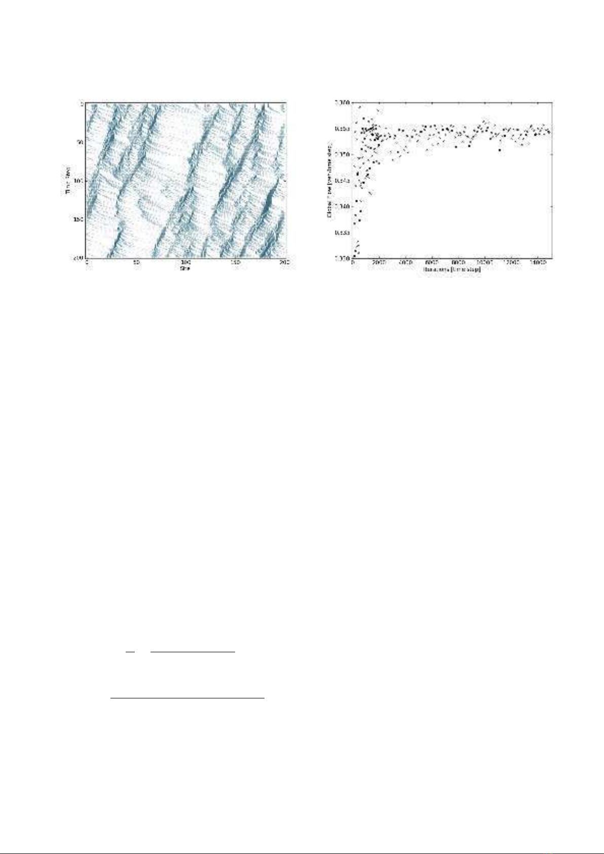
FIG. 1: A space-time diagram for the NaSch Model with L=
200, p= 0.5, ρ= 0.5, and 200 time steps. Vehicles are moving
to the right, and traffic jams to the left. Darker points indicate
a lower the velocity of the vehicle on the road. A white ‘data
point’ indicates the lack of a vehicle.
responds to an actual length of 1500m (each site being
7.5m in length). 200 time steps, where each time step
is approximately 1 second (an approximation of the re-
action time of a driver), and vmax = 5 where this corre-
sponds to an actual velocity of 120kmh−1were also used.
The vehicles were distributed randomly along with road
with randomly assigned velocities from zero to vmax = 5.
Figure 1shows the space-time diagram for the aforemen-
tioned conditions with 50 vehicles occupying the road.
It can be seen that vehicles are moving to the right with
each time step and the darker the point on the space-time
diagram, the lower the velocity. The darkest parts of this
graph are jams (with velocity v= 0), and move in the
opposite direction to the vehicles direction of travel. This
phenomenon is produced as a vehicle is not affected by
the traffic behind it (due to rule 2 in the NaSch model),
and hence, causality travels in the opposite direction.
To produce an average velocity vs. global density dia-
gram, and the fundamental (density-flow) diagrams, the
global flow and global density need to be calculated. The
global density, ρ, and global flow, J(ρ), are defined by
equations 1and 2respectively.
ρ=N
L=Number of vehicles
Number of sites (1)
J(ρ) = Number of vehicles passing a point
Number of time steps (2)
Due to the random initial distribution of vehicles,
global flow is calculated after the initial step due to the
initial random configuration needing to settle. The fun-
damental diagrams were plotted for L= 200, with 200
FIG. 2: The number of iterations vs. global flow with L=
200, p= 0.5, and vmax = 5. When flow is calculated for a
low number of iterations, large errors are observed without
the need for statistical analysis.
iterations, vmax = 5 and varying density ρ, in steps of
δρ = 0.01. However, due to the fluctuations in the cal-
culated flow it was necessary to create a global flow vs.
iterations graph to find an ideal number of iterations for
L= 200 as seen in figure 2. Observations by eye were
sufficient and determined 10000 iterations to be an ap-
propriate value to use with respect to accuracy and com-
putational time (for more information refer to Appendix
C).
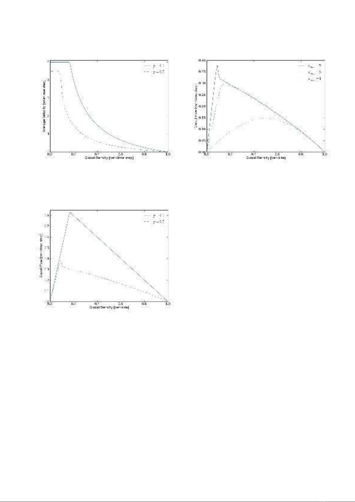
The first study using the NaSch model was to plot av-
erage velocity, hvi, vs. global density, ρ, for two different
values of p. It can be seen in figure 3that for both val-
ues of pthere is a critical density at which the average
velocity is no longer equal to vmax . The flow drops off
quickly at the critical density as one would expect. It is
also able to show that for a larger value of pthe average
velocity of the system collapses at a lower density, and
in reality increases the chance of collisions. This increase
in pvia a constant distraction explains the need for the
Department of Transport to introduce preventative mea-
sures against rubbernecking [5]. The results agree with
the observations of an actual road [1], and the same pat-
tern is shown for different values of vmax [6]. This allows
one to initially determine the maximum density of a road
for best flow.
Figures 4and 5show the fundamental (density-flow)
diagrams for changing pand vmax respectively. With in-
creasing vmax the dynamics change considerably; note
that the relationship for vmax = 1 is symmetric due
to particle-hole symmetry [7], and this is broken at
vmax >1. The maximum flow tends from rounded to a
sharp point with the increase of vmax due to the smaller
range of velocities. For figure 4, increasing pleads to
higher fluctuations in velocities and separation between
successive vehicles, which in turn results in the collapse
3
FIG. 3: Average Velocity, hvi, vs. Global Density, ρ, with
L= 200, 200 iterations, vmax = 5 and varying density ρ,
with δρ = 0.01
FIG. 4: A fundamental density-flow diagram for the NaSch
model with L= 200 sites, vmax = 5, and δρ = 0.01 and vary-
ing p. Measurements were mean measurements over 10000
time steps.
in the flow at lower densities as predicted by figure 3. For
an arbitrary value of p, and very low values of ρ,ρ→0,
the flow of traffic is very low, J(ρ)→0. This can be ex-
plained by the low number of vehicles occupying the road,
such that nearly no flow exists. As ρ→1, J(ρ)→0 be-
cause vehicles can hardly move forward. This allows the
flow of a given road to successfully predicted from only
the global density, the maximum velocity, and the decel-
eration probability. The physical implications of these
regions will be studied in more detail in the following
section.
It should also be noted that while figures 4and 5agree
with T. Held, et al [8], and also general trends obtained
FIG. 5: A fundamental density-flow diagram for the NaSch
model with L= 200 sites, p= 0.5, and δρ = 0.01 and varying
vmax . Measurements were mean measurements over 10000
time steps.
by J. Whale, et al [2] there is a slight variation in global
flow for vmax = 5, ρ= 0.5, at the point of maximum
flow. This can be explained as the graphs here were pro-
duced using L= 200, and as a result are affected by the
finite size of the road. A system of L= 10000 would
be sufficient to exclude these effects [9] but as a conse-
quence uses significantly more computational time (see
Appendix B).
More detailed measurements involving road traffic
[10][11][12][13] yield the result that flow is not a unique
function of density, as these fundamental diagrams sug-
gest. A simple extension of the NaSch model in the next
section will update the model to account for such find-
ings. Regardless, the NaSch model is sufficient to model
traffic [1] and allows predictions to be made about the
maximum flow of a given road, and consequences of ve-
hicle behaviour [2].
4. THE
VELOCITY-DEPENDENT-RANDOMISATION
(VDR) MODEL
Two types of jams are possible. There are jams that
are induced by an external circumstance, such as a bot-
tleneck or lane reductions, and also the spontaneous jams
which are caused by fluctuations in vehicle velocities.
Spontaneous jams were first shown by T. Treiterer [14]
who examined a series of aerial photographs of a high-
way and it was also shown by B. S. Kerner, et al [15]
that phase separated jams and homogeneous metastable
states exist. The original NaSch model studied until now
doesn’t exhibit metastable states or hysteresis. Nor does
it exhibit spontaneous, wide phase-separated jams. With
a small extension to the original model it is possible to
4
reproduce these phenomena. This is the VDR model
(Barlovic et al [16]) and is based on the NaSch model
but with the addition of a slow-to-start rule.
In the VDR model the deceleration parameter, pn(vn),
depends on the velocity, vn, of a vehicle, n. This parame-
ter is calculated in an initial step (now called step 0) and
subsequently used in step 3 of the NaSch model. The
rule is as follows
0. Determination of the randomisation parameter pn,
for vehicle n:
pn(vn) = p0for vn= 0
pfor vn>0
This is the slow-to-start rule, with two stochastic pa-
rameters p0and pwhich allow the aforementioned phe-
nomena to be reproduced. If a vehicle is stationary
(vn= 0) then the vehicle has a probability p0that it
will not accelerate to vn= 1 in following time step.
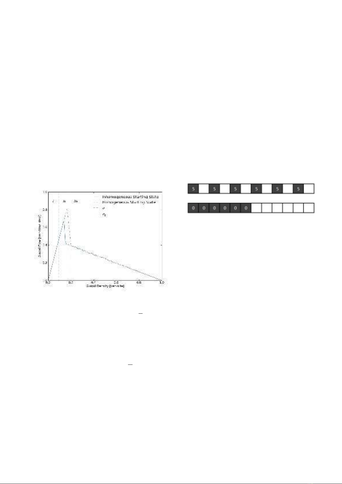
FIG. 6: The fundamental (density-flow) diagram for the VDR
model, plotting for homogeneous and inhomogeneous starting
conditions with L= 200 sites, vmax = 5, p=1
64 ,p0= 0.75,
and flow averaged over 10000 iterations. The peak of the
inhomogeneous branch is due to finite length effects of the
road discussed in Appendix C, and is accounted for by the
location of ρ1.
In this part of the investigation I consider the VDR
model with the same parameters as in the NaSch model,
but with a deceleration probability p=1
64 for the moving
vehicles, and p0= 0.75 for the vehicles at rest (vn= 0),
and with the addition of the above step. It should be
noted that p0≫p. The inverse of this will produce
significantly different results and p0=preproduces the
original NaSch model.
The simulation was implemented for two starting con-
ditions. A homogeneous state, in which all vehicles
are equally separated with vmax , and an inhomogeneous
state, in which the vehicles are all jammed with vn= 0
(see figure 7).
The typical fundamental diagram (figure 6) of the
VDR model shows three important regions. Region I,
in which ρ < ρ1, is a free flow regime. For densities up to
the ρ1no jams with a long lifetime appear [17], and jams
that exist in the initial road condition quickly disappear
since the outflow from the jam is larger than the inflow
(see figure 1). In contrast, in region III, where ρ > ρ2,
a homogeneous state without jams cannot occur. For
region II, the flow J(ρ) can take on two different states
depending on the initial conditions mentioned previously.
One is a homogeneous free-flow metastable branch with a
long lifetime [8], and the other is a jammed branch with
phase separation between the jammed and free-flowing
vehicles.
The microscopic structure of the jammed state seen in
the VDR model is different to observed jammed states
in the NaSch model. The NaSch model contains jammed
states with exponential size distribution [18], however,
the VDR model shows phase separation.
FIG. 7: The homogenous starting state of a road at which all
vehicles start equally distant with vmax , and the inhomoge-
neous starting state of the road where all vehicles are jammed
with a velocity v= 0. This situation is demonstrated for a
length L= 12, and ρ= 0.5
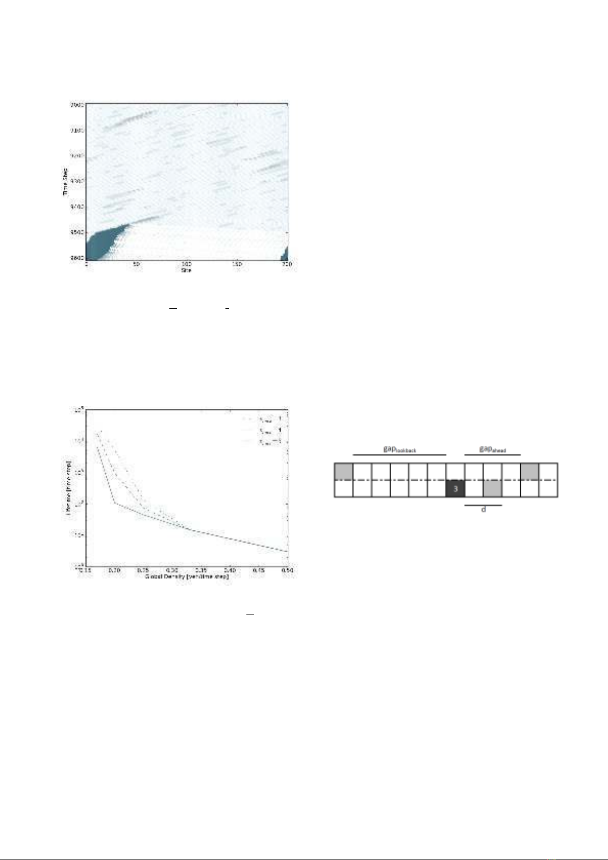
The appearance of a spontaneous, wide phase-
separated jam can be seen in figure 8which is able to
show that the density in the outflow region of the jam
is reduced compared to the global density. This allows
the jam length to grow approximately linearly until the
outflow and inflow are in equilibrium (a result of periodic
boundary conditions). The jam is formed due to a veloc-
ity fluctuation after starting in the homogeneous state.
The velocity fluctuation of a single vehicle can cause the
vehicle behind to reduce its velocity when the gap be-
tween them becomes small (d≤vn). If the density in
the area concerned is large enough this leads to a chain
reaction which in turn causes a vehicle to stop, and a jam
to form. The time taken for this to happen is the lifetime
of the metastable state, τ.
The lifetime of the metastable state is shown in figure
9where a jam is defined by three stopped vehicles in
a row. It is observed that with the decrease in density
the lifetime of the metastable state increases with a more
than exponential rate. For a given density, for example
ρ= 0.2, small values of vmax can lead to lifetimes which
are greater by orders of magnitude than higher vmax.
A system could be implemented in which if a road is
found to be in a metastable state the maximum velocity
is reduced, therefore reducing the probability of a jam
occuring and postponing the inevitable collapse of the
5
FIG. 8: The spontaneous formation of a jam for L= 200,
vmax = 5, p= 0.75, p0=1
64 , and ρ=1
6. The darker the
point, the lower the velocity, and a white ‘data point’ indicates
an empty cell. The homogeneous lifetime is approximately
9450 time steps in this example.
FIG. 9: The lifetime of the metastable state (log scale) vs.
Global Density, with L= 200, p= 0.75, p0=1
64 ,δρ = 0.01,
and varying vmax , plotted for means of 100 measurements.
flow into the jammed branch as shown in figure 8.
There are numerous possibilities to extend the VDR
model. A distraction in an adjacent lane, the effects
of traffic lights or on-off ramps have all been previously
studied [8] however, in the next section a two-lane model
will be developed.
5. THE DEVELOPMENT OF A TWO LANE
MODEL
It is necessary to choose an appropriate lane-changing
rule set depending on the situation of the experiment.
First I consider symmetric lane changing rules which are
relevant for US highways and traffic in towns, in which
overtaking on both lanes is allowed. The asymmetric rule
set describes motorways in the UK, and other European
countries. This rule set effectively divides the system into
a ‘slow’ and ‘fast’ lane, left and right lanes respectively.
According to the standard set of lane changing rules by
other authors, notably [19][20][21][22], the lane changing
rules for a symmetric road are as follows.
1. Incentive criterion: If vn≥dit would be more
beneficial to transfer lanes (and remain at vnrather
than braking as in the NaSch model).
2. Safety criterion: For a vehicle to transfer to the
adjacent lane, the adjacent site must be unoccupied
with gaplookback =vmax and gapahead =vn.
For an asymmetric road, an additional rule, before the
‘Incentive criterion’ is also present.
0. Intuition step: A vehicle prefers to be in the left
lane (slow lane).
These rules then replace rule 2 of the NaSch model.
FIG. 10: An example of the two-lane model with vehicles
moving to the right. The dark grey hatched cell is the vehicle
attempting to change from the right, to left lane (with vn=
3), while the light grey hatched cells are other vehicles on the
two-lane road
An example of the conditions being satisfied is given in
figure 10. The first of the lane changing rules is due to a
vehicle approaching another vehicle from behind. In the
NaSch model this vehicle would decelerate (vn=d−1),
but here, it is given the opportunity, as long as the second
rule is satisfied, that it can change lanes and carry on at
the same velocity, vn. The second rule assures a vehicle
can initially get into the adjacent lane and makes sure
that a vehicle has enough space behind it to pull out and
not cause a collision or excessive deceleration with a ve-
hicle travelling at vn=vmax. It also checks that there is
enough space ahead such that it can move forward with-
out the same consequences. After these steps have taken
place the normal NaSch rule set is then implemented to
move traffic forward in time.


![Gia Công & Lắp Đặt Cốt Thép: Kỹ Thuật Xây Dựng Bê Tông [Chuẩn Nhất]](https://cdn.tailieu.vn/images/document/thumbnail/2026/20260531/alfredodistefano10/135x160/58891780257145.jpg)
![Gia Công Ván Khuôn: Lắp Dựng, Tháo Dỡ và Kỹ Thuật Xây Dựng [Chi Tiết A-Z]](https://cdn.tailieu.vn/images/document/thumbnail/2026/20260531/alfredodistefano10/135x160/4261780257147.jpg)

![Giáo Trình Công Tác Xây Dựng: Kỹ Thuật và Vật Liệu Xây Dựng [A-Z]](https://cdn.tailieu.vn/images/document/thumbnail/2026/20260531/alfredodistefano10/135x160/9351780261637.jpg)


%20--%3e%3cdefs%3e%3cstyle%3e%20.st0%20{%20fill:%20%23fff;%20}%20.st1%20{%20fill:%20%237800fa;%20}%20%3c/style%3e%3c/defs%3e%3cpath%20class='st1'%20d='M117.78,12.18H43.11c2.9,3.47,4.65,7.94,4.65,12.82,0,5.6-2.3,10.66-6.01,14.29h76.02l7.22-13.56-7.22-13.56Z'/%3e%3cg%3e%3cpath%20class='st0'%20d='M53.58,26.17h-.59v-1.46h.59v-4.96h2.83c1.78,0,2.67.94,2.67,2.82v5.76c0,1.87-.89,2.81-2.67,2.81h-2.83v-4.96ZM55.36,21.37v3.34h1.1v1.46h-1.1v3.34h1.01c.61,0,.91-.37.91-1.1v-5.93c0-.74-.3-1.1-.91-1.1h-1.01Z'/%3e%3cpath%20class='st0'%20d='M65.99,31.14h-1.8l-.31-2.07h-2.19l-.31,2.07h-1.64l1.82-11.39h2.62l1.82,11.39ZM65.28,18.04c-.25.46-.51.77-.75.94-.21.15-.47.22-.79.22-.26,0-.57-.07-.92-.22l-.38-.15c-.14-.05-.26-.07-.37-.07-.3,0-.53.18-.71.54l-.91-.68c.25-.46.51-.77.75-.94.21-.14.48-.21.79-.21.26,0,.57.07.92.21l.38.15c.14.05.26.07.37.07.3,0,.53-.18.71-.54l.91.68ZM61.91,27.52h1.73l-.87-5.76-.87,5.76Z'/%3e%3cpath%20class='st0'%20d='M74.53,26.89v1.52c0,1.91-.89,2.86-2.67,2.86s-2.67-.95-2.67-2.86v-5.93c0-1.91.89-2.86,2.67-2.86s2.67.95,2.67,2.86v1.11h-1.69v-1.22c0-.75-.31-1.12-.93-1.12s-.93.37-.93,1.12v6.15c0,.74.31,1.11.93,1.11s.93-.37.93-1.11v-1.63h1.69Z'/%3e%3cpath%20class='st0'%20d='M81.4,31.14h-1.8l-.31-2.07h-2.19l-.31,2.07h-1.64l1.82-11.39h2.62l1.82,11.39ZM75.9,19.2l1.52-1.91h1.71l1.51,1.91h-1.61l-.76-.95-.75.95h-1.61ZM77.32,27.52h1.73l-.87-5.76-.87,5.76ZM83.1,15.99l-1.76,1.91h-1.26l1.17-1.91h1.86Z'/%3e%3cpath%20class='st0'%20d='M84.86,19.75c1.78,0,2.67.94,2.67,2.82v1.48c0,1.87-.89,2.81-2.67,2.81h-.85v4.28h-1.79v-11.39h2.64ZM84.01,21.37v3.86h.85c.58,0,.87-.36.87-1.08v-1.71c0-.71-.29-1.07-.87-1.07h-.85Z'/%3e%3cpath%20class='st0'%20d='M93.51,19.75c1.78,0,2.67.94,2.67,2.82v1.48c0,1.87-.89,2.81-2.67,2.81h-.85v4.28h-1.79v-11.39h2.64ZM92.66,21.37v3.86h.85c.58,0,.87-.36.87-1.08v-1.71c0-.71-.29-1.07-.87-1.07h-.85Z'/%3e%3cpath%20class='st0'%20d='M98.8,31.14h-1.79v-11.39h1.79v4.88h2.03v-4.88h1.83v11.39h-1.83v-4.88h-2.03v4.88Z'/%3e%3cpath%20class='st0'%20d='M105.36,24.55h2.46v1.62h-2.46v3.34h3.09v1.63h-4.88v-11.39h4.88v1.63h-3.09v3.18ZM108.17,17.29l-1.76,1.91h-1.26l1.17-1.91h1.86Z'/%3e%3cpath%20class='st0'%20d='M112.2,19.75c1.78,0,2.67.94,2.67,2.82v1.48c0,1.87-.89,2.81-2.67,2.81h-.85v4.28h-1.79v-11.39h2.64ZM111.35,21.37v3.86h.85c.58,0,.87-.36.87-1.08v-1.71c0-.71-.29-1.07-.87-1.07h-.85Z'/%3e%3c/g%3e%3ccircle%20class='st1'%20cx='25'%20cy='25'%20r='20'/%3e%3cpath%20class='st0'%20d='M32.78,19.27c2.92,0,4.43,2.55,5.28,5.33l.71,2.17c.14.38-.33.75-.71.75h-5.61c.19-.33.24-.71.09-1.08l-.75-2.45c-.43-1.32-.99-2.64-1.79-3.77.75-.57,1.65-.94,2.78-.94h0ZM25,18.38c3.25,0,4.9,2.78,5.89,5.89l.76,2.45c.14.42-.33.8-.8.8h-11.69c-.42,0-.94-.38-.8-.8l.75-2.45c.99-3.11,2.64-5.89,5.89-5.89h0ZM25,11.35c1.74,0,3.11,1.37,3.11,3.11s-1.37,3.11-3.11,3.11-3.11-1.41-3.11-3.11,1.41-3.11,3.11-3.11h0ZM17.27,19.27c1.08,0,1.98.38,2.73.94-.8,1.13-1.37,2.45-1.74,3.77l-.8,2.45c-.14.38-.05.75.09,1.08h-5.56c-.42,0-.9-.38-.75-.75l.71-2.17c.9-2.78,2.41-5.33,5.33-5.33h0ZM17.27,12.91c1.51,0,2.78,1.27,2.78,2.83s-1.27,2.83-2.78,2.83-2.83-1.27-2.83-2.83,1.27-2.83,2.83-2.83h0ZM32.78,12.91c1.56,0,2.78,1.27,2.78,2.83s-1.23,2.83-2.78,2.83-2.83-1.27-2.83-2.83,1.27-2.83,2.83-2.83h0ZM27.07,28.56v.09c0,.57-.24,1.08-.61,1.46h0v.05c-.38.33-.9.57-1.46.57s-1.08-.24-1.46-.61h0c-.38-.38-.61-.9-.61-1.46v-.09h1.41v.09c0,.19.05.38.19.47v.05c.09.09.28.19.47.19s.38-.09.47-.19v-.05c.14-.09.24-.28.24-.47t-.05-.09h1.41ZM30.99,28.56v.09c0,1.65-.66,3.16-1.74,4.24-1.08,1.08-2.59,1.79-4.24,1.79s-3.16-.71-4.24-1.79l-.05-.05c-1.04-1.08-1.7-2.55-1.7-4.2v-.09h1.41v.09c0,1.27.47,2.4,1.27,3.25h.05c.85.85,1.98,1.37,3.25,1.37s2.4-.52,3.25-1.37c.85-.8,1.37-1.98,1.37-3.25v-.09h1.37ZM34.99,28.56v.09c0,2.78-1.13,5.28-2.92,7.07-1.79,1.79-4.29,2.92-7.07,2.92s-5.23-1.13-7.07-2.92c-1.79-1.79-2.92-4.29-2.92-7.07v-.09h1.41v.09c0,2.4.94,4.53,2.5,6.08,1.56,1.56,3.72,2.5,6.08,2.5s4.52-.94,6.08-2.5c1.56-1.56,2.5-3.68,2.5-6.08v-.09h1.41Z'/%3e%3c/svg%3e)