
REGULAR ARTICLE
Modeling and control of xenon oscillations in thermal
neutron reactors
Bertrand Mercier
1,*
, Zeng Ziliang
2
, Chen Liyi
2
, and Shao Nuoya
2
1
CEA/INSTN, 91191 Gif sur Yvette, France
2
Institut Franco-Chinois de l’Energie Nucléaire, Sun Yat-sen University, 519082 Zhuhai Campus, Guangdong Province,
P.R. China
Received: 18 November 2019 / Received in final form: 3 March 2020 / Accepted: 12 March 2020
Abstract. We study axial core oscillations due to xenon poisoning in thermal neutron nuclear reactors with
simple 1D models: a linear one-group model, a linear two-group model, and a non-linear model taking the
Doppler effect into account. Even though nuclear reactor operators have some 3D computer codes to simulate
such phenomena, we think that simple models are useful to identify the sensitive parameters, and study the
efficiency of basic control laws. Our results are that, for the one-group model, if we denote the migration area by
M
2
and by Hthe height of the core, the sensitive parameter is H/M.Hbeing fixed, for the 2 groups model, there
are still 2 sensitive parameters, the first one being replaced by M2
1þM2
2where M2
1denotes the migration area for
fast neutrons and M2
2the migration area for thermal neutrons. We show that the Doppler effect reduces the
instability of xenon oscillations in a significant way. Finally, we show that some proportional/integral/
derivative (PID) feedback control law can damp out xenon oscillations in a similar way to the well-known
Shimazu control law [Y. Shimazu, Continuous guidance procedure for xenon oscillation control, J. Nucl. Sci.
Technol. 32, 1159 (1995)]. The numerical models described in our paper have been applied
to PWR.
1 Introduction
A lot of publications can be found in the literature on
the problem of xenon oscillations in nuclear reactors
[1–10].
As reported in [1] xenon oscillations have occurred in
Savannah River as early as in 1955.
The fact is that 54
135Xe is the fission product with the
highest capture cross section and that it can be produced
either directly or via beta-decay of another fission product
which is 54
135I.
Axial core oscillations have been first studied with two
zones lumped models, and then by a one group diffusion
model coupled to the evolution equations for xenon and
iodine.
The first question is whether we should use a
time dependent diffusion equation like in [11]ora
stationary diffusion equation like in [1] and many other
References
With the former approach, we benefit from theoretical
results on the Hopf bifurcation on non linear systems. With
the latter it seems possible to prove theoretical results on
the linearized system only.
More precisely, mathematical criteria have been found
for the sign of the real part of the eigenvalues of the
linearized system (see e.g. [4]).
Physically, there are at least three time scales in the
core of a nuclear reactor: the prompt neutrons life time
(∼20 ms), the delayed neutrons time scale (∼1 s), and the
time scale for xenon oscillations (∼5 h).
A two-group time-dependent model taking the delayed
neutrons into account is described in Ponçot’s thesis [10].
Practically, in a PWR, criticality of the core is ensured
by adjusting either the Boron concentration or by using
the control rods. At the time scale of xenon oscillations, we
can assume that the core is critical, so that there is no need
to consider a time-dependent equation for the neutron
flux.
Rather, at each time step, the xenon concentration
being given, it is appropriate to solve an eigenvalue
problem.
The second question is whether we should use a one-
group model or a two-group model (one group for fast
neutrons, one group for thermal neutrons) like the one
considered in [10].
*e-mail: bertrand.mercier@cea.fr
EPJ Nuclear Sci. Technol. 6, 48 (2020)
©B. Mercier et al., published by EDP Sciences, 2020
https://doi.org/10.1051/epjn/2020009
Nuclear
Sciences
& Technologies
Available online at:
https://www.epj-n.org
This is an Open Access article distributed under the terms of the Creative Commons Attribution License (https://creativecommons.org/licenses/by/4.0),
which permits unrestricted use, distribution, and reproduction in any medium, provided the original work is properly cited.

Indeed, since the xenon capture cross section is
significant for thermal neutrons only, one might think
that it is more appropriate to introduce a two-group
model.
In the present paper, we show that it is possible to
derive a one-group model with the same behavior as our
two-group model provided that, in the one-group model,
the diffusion equation holds for the thermal neutron flux
only and that the migration area is selected in an adequate
way.
We show that for both one-group and two-group
models, the height of the core and the magnitude of the
neutron flux are sensitive parameters.
In [12], we have shown that, as far as xenon oscillations
are concerned, introducing a reflector is equivalent to
increasing the height of the core.
After showing that the one-group model is possible, we
add a nonlinear term in the diffusion equation to take the
Doppler effect into account: like in [1], we find that it helps
damping out the oscillations.
Finally, we address the question, which is of primary
importance, of how to better control the oscillations.
We test the well-known Shimazu control law [13–15].
We check that it is efficient as expected, but we show
that a PID control strategy can also be applied.
Our models are presented in a mathematical way, and
we use adequate rescaling methods both to reduce the
number of parameters and to facilitate their application
(which is outside the scope of this work) to other thermal
neutron reactors like CANDU or HTR. The results we show
below are related to PWR.
2 The 1 group diffusion model
According to the neutron transport theory and the
diffusion theory, the one group diffusion equation for a
homogeneous reactor can be written, in the uniaxial case,
as:
M2F00 þF¼k∞F;0<z<H;ð1Þ
where His the height of the core. Fis the neutron flux of the
core in n/cm
2
/s and M
2
denotes the migration area in cm
2
.
This differential equation should be completed by some
boundary conditions (BC). In the following we shall choose
the Dirichlet BC:
Fð0Þ¼FðHÞ¼0:ð2Þ
We refer the reader to [3] for the Fourier BC.
In a one group model, the migration area is arbitrarily
evaluated by taking into account both fast and thermal
neutrons.
In the present section which is dedicated to the
one-group model, the solution Fto equation (2) will
be assumed to be the thermal neutron flux in the
core.
We remind the reader that (1) and (2) is an eigenvalue
problem and then that Fis defined up to a multiplicative
factor.
2.1 Introduction of iodine and xenon
We have the following evolution equations:
dY
dt ¼gSfFlY;ð3Þ
dX
dt ¼g0SfFþlYðmþsFÞX;ð4Þ
where:
–Y(resp. X) is the concentration of 53
135I(resp. 54
135Xe) in the
fuel evaluated in at/cm
3
of fuel;
–sis the microscopic capture cross section for xenon in the
thermal domain (evaluated in barns);
–S
f
is the macroscopic fission cross section of the fuel in
the thermal domain;
–gthe iodine fission yield (about equal to 0.064 for UO2
fuel);
–g
0
the xenon fission yield (about equal to 0.001 for UO2
fuel);
–l(resp. m) the time constant for the bdecay of 53
135I
(resp. 54
135Xe).
For the sake of simplicity, in the following, we shall
neglect xenon generation from fission reaction directly,
which is possible since g
0
≪g.
Note that in (3) and (4) S
f
is evaluated in cm
1
and F
in n/cm
2
/s.
The core is assumed to be homogenized so that, in each
cm
3
of core, there are vcm
3
of fuel and (1 v)cm
3
of
moderator. In a PWR we have v∼1/3 so that the
moderation ratio (1 v)/v∼2.
Since there are vXat/cm
3
of 54
135Xe in the core, the
xenon macroscopic cross section is equal to vsXOnce
taking into account the neutron capture by 54
135Xe equation
(1) has to be replaced by
M2∂2
∂z2Fþð1þaXÞF¼k∞F;0<z<H;ð5Þ
where a=vs/Sand Sis the absorption cross section of the
core.
In view of (3) and (4) we shall have Y=Y(z, t), X=X(z, t)
and then F=F(z, t)from(5).
2.2 Rescaling of the one group model
Following [16] we let
Fðz;tÞ¼F’ðz;tÞ;
Xðz;tÞ¼Xxðz;tÞ;
Yðz;tÞ¼Yyðz;tÞ:
We also replace tby t=lt, and we let F
=l/s,a=m/l
and X¼gSfF
l¼gSf
s. We get the simpler system
2 B. Mercier et al.: EPJ Nuclear Sci. Technol. 6, 48 (2020)

dy
dt¼’y;ð6Þ
dx
dt¼yðaþ’Þx:ð7Þ
Finally, let a¼aX¼vs
S:gSf
s¼v:gSf
S, we get
M2∂2
∂z2’þð1þaxÞ’¼k∞’;0<z<H:ð8Þ
X
has the following interpretation: it is the equilibrium
value for the concentration of
135
Xe atoms when the
neutron flux is infinitely large.
Equations (6)–(8) completed with Dirichlet BC is the
one-group system which we shall solve.
We could have also changed the space variable z→Z/M
to prove that the main parameter is H/M.
Typical values of the parameters to be selected for
PWR reactors are shown in Table 1.
2.3 Space approximation
We introduce a discretization step Dz=H/(N+1) where N
is the number of discretization points. We now denote by ’
the column-vector of values or the rescaled thermal
neutron flux at the discretization points iDz, 1iN.
(Our numerical results will be obtained with N= 39, but
this is not a sensitive parameter.)
We introduce the tridiagonal matrix Asuch that
ðA’Þi¼ð’i1þ2’i’iþ1Þ=Dz2;
where we assume that ’
0
= 0 and ’
N+1
= 0 which
corresponds to the Dirichlet boundary conditions.
We shall make the following convention : (x’)
i
=x
i
’
i
,
which means that, depending on the context xmay
denote either a vector in ℝ
N
or the NNdiagonal matrix
containing the components of xon its main diagonal.
Let {y
∞
,x
∞,
’
∞
} be a steady solution of (6)–(8)
satisfying
ðaþ’∞Þx∞¼y∞¼’∞;ð9Þ
M2A’∞þð1þax∞Þ’∞¼k∞’∞:ð10Þ
We note that the solution {y
∞
,x
∞,
’
∞
}of(9) and (10)
cannot be unique: in fact x
∞
being given, (10) is an
eigenvalue problem (which means that the core is critical)
so that ’
∞
is defined up to a multiplicative constant and we
fix this constant so that the core power is given.
In the case where our steady solution {y
∞
,x
∞,
’
∞
}is
not stable, if we start from {y
a
,x
a
} close to {y
∞
,x
∞
}we
shall activate an oscillation. This means that the reactor
core is unstable.
2.4 Time discretization: semi implicit scheme
We denote the time step by d. We let t
n
=nd.
We use the following semi implicit scheme:
First step, solve
ynd’
n1yn
yn1¼0;
xndynðaþ’n1Þxn
xn1¼0:
Second step, solve
M2AþðIþaxnÞ
’n¼k∞’n:
Which produces both a value for kn
∞(the smallest
eigenvalue) and a (non-unique) value for ’
n
.
Then we replace ’
n
by ’ntimes ’=averageð’nÞ, where ’
is a prescribed value for the average of the (normalized)
flux.
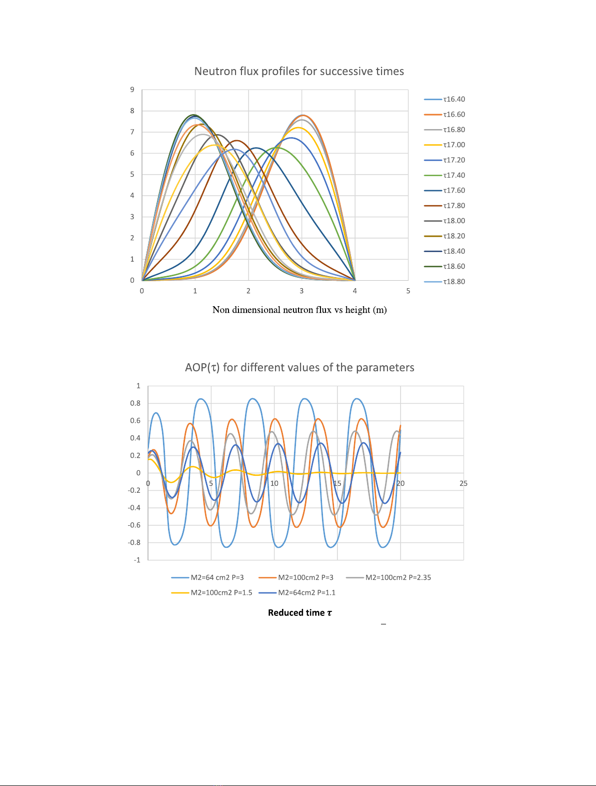
2.5 Results with the one group model
When the average flux is sufficiently high the flux
oscillations are first growing and then stabilize.
A typical result is given in Figure 1 for which ’¼3,
which is a rather high value since 3F
*
= 4.38
10
13
n/cm
2
/s.
To illustrate the evolution of the oscillations we shall
use the Axial Offset AO
p
defined by AO
p
=(P
t
P
b
)/
(P
t
+P
b
) where P
t
(resp. P
b
) is the average power (or
neutron thermal flux) in the upper (resp. lower) half part of
the core.
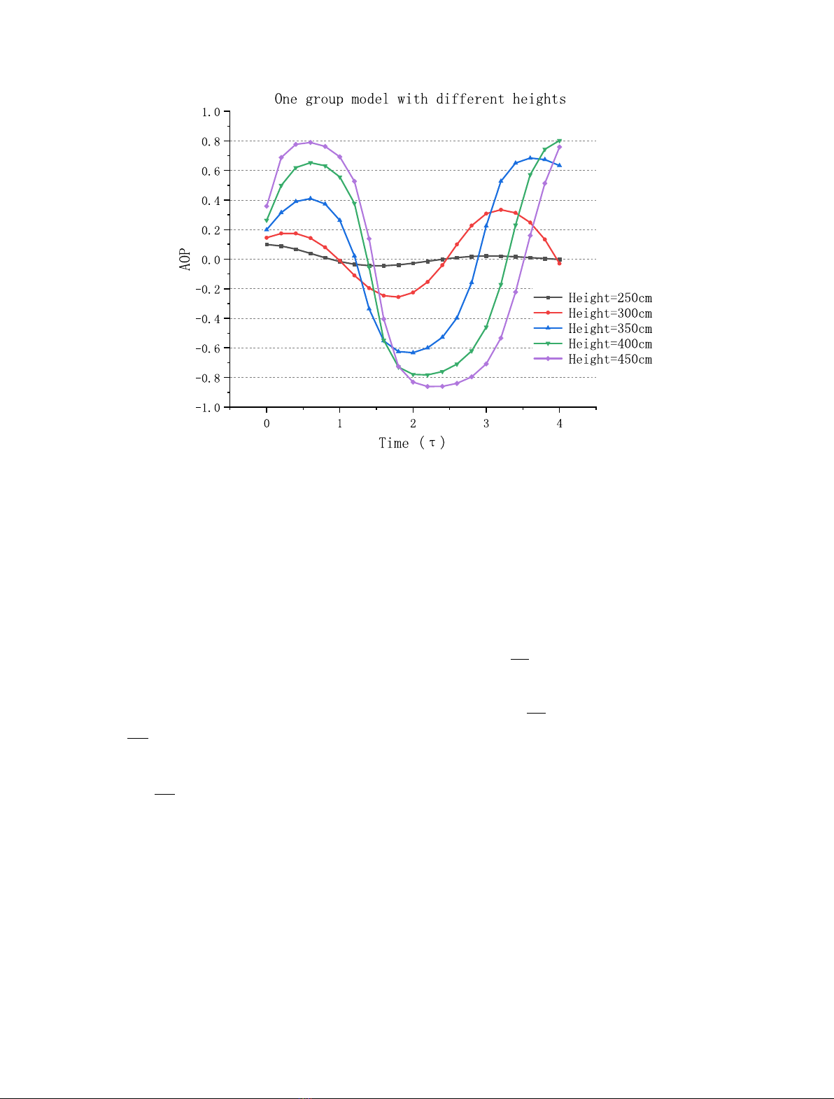
Figure 2 shows the evolution of AO
p
with the reduced
time t.
We see that the oscillations are
–damped out when M
2
=100 cm
2
and ’¼1:5;
–stable when M
2
=64 cm
2
and ’¼1:1;
–growing when M
2
=100 cm
2
and ’¼2:35 or 3 or M
2
=
64 cm
2
and ’¼3.
When the oscillations are growing they reach a limit
cycle, and this is because we ensure criticality at all times.
Now from the operator’s point of view these oscillations are
instabilities.
On a standard PWR we know that the migration area is
more like 64 cm
2
. Note that the period of oscillations
depends both on the migration area and on ’: it can
range between 28 and 36 h, which is consistent with the
measurements made in actual PWR [17](∼30 h for a
900 MWe [5]).
Table 1. Typical numerical data for our one-group model
(see [11] p. 382).
l2.92 10
5
s
1
S
f
0.246 cm
1
m2.12 10
5
s
1
S0.115 cm
1
a0.725 F1.459 10
13
n/cm
2
/s
g0.064 Y
*
7.87 10
15
at/cm
3
s210
6
barns X
*
7.87 10
15
at/cm
3
v1/3 a
0.0452
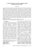
B. Mercier et al.: EPJ Nuclear Sci. Technol. 6, 48 (2020) 3
In Figure 3 we show the influence of the height of the
core on the oscillations.
When the reactor core is lower than 250 cm, no
oscillation is activated. Once the height is more than
300 cm, a growing oscillation can be produced. Moreover,
the higher the height is, the bigger AO
p
is.
3 The 2-group model
There are many neutrons with different energy in a reactor
core. It is usually considered that the fast neutrons possess
an energy more than 0.625 eV, and on the contrary, that
the thermal neutrons have an energy less than 0.625 eV.
Fig. 1. The oscillation of neutron flux in 1 group model with M
2
=64 cm
2
.
Fig. 2. Evolution of the axial offset AO
p
for various values of ’¼Pand M
2
= M2.
4 B. Mercier et al.: EPJ Nuclear Sci. Technol. 6, 48 (2020)
Applying the data in [11], the thermal neutron flux is
equal to 3.7 10
13
n/cm
2
/s in average in the fuel pins of a
PWR. In addition, the fast neutron flux is almost 7 times as
high as the thermal neutron flux. It’s then approximately
equal to 2.7 10
14
n/cm
2
/s in average in the fuel. Even
though the highest flux in a PWR core corresponds to the
fast domain, more than 80% of the fissions happen in the
thermal domain. For a 1300 MWe PWR, there are
about 1.1 10
13
fissions/cm
3
/s in the fuel at nominal
power (3800 MWth).
Let C(resp. F) denote the fast (resp. thermal) neutron
flux, we shall use the following system of coupled diffusion
equations
D1
∂2
∂z2CþS1C¼nvSf2FþnvSf1C;ð11Þ
D2
∂2
∂z2FþS2FþvsXF¼pS1C:ð12Þ
Like in Section 2,vsXis the xenon macroscopic capture
cross section : it should be added to S
2
.
In the same way, if S
f1
(resp. S
f2
) denotes the
macroscopic fission cross section of the fuel in the fast
(resp. thermal) neutron domain, vS
f1
C(resp. vS
f2
F)
denotes the number of fast (resp. thermal) fission per cm
3
per s in the core.
Note that the xenon capture cross section is negligible
for fast neutrons.
Now, S
1
Cis the number of fast neutrons which
disappear per cm
3
per s. Some of them are physically
absorbed but a fraction pof them reappear, after slowing
down, in the thermal neutron group.
The factor pappears to be the resonance escape
probability from Enrico Fermi’s four factors formula.
For the sake of simplicity, we shall assume that the
diffusion coefficients do not depend on the space variable z.
Even though (11) and (12) are stationary diffusion
equations, we may have X=X(z, t).
The xenon evolution is coupled to the iodine evolution
through
dY
dt ¼gSf1CþSf2F
lY;ð13Þ
dX
dt ¼lYðmþsFÞX:ð14Þ
Such an evolution is rather slow at the scale of one hour,
so there is no need to consider the neutron evolution at the
timescale of delayed neutrons.
The 2 groups model will be complemented by some
boundary conditions for the neutron flux.
We shall mainly consider the Dirichlet boundary
conditions
Cð0Þ¼CðHÞ¼Fð0Þ¼FðHÞð15Þ
but it is also possible to consider the Fourier boundary
conditions.
Remark: The number of neutrons produced by fast
fission of 92
235Uis actually 2.8, but, for the sake of simplicity,
we choose n= 2.4 both for 92
238Uand 92
235U. However, it
would be easy to change the term nvS
f1
Cin (11) by
n
1
vS
f1
Cwhere n
1
is some appropriate average of 2.4
and 2.8.
Fig. 3. Evolution of AO
p
for various values of height.
B. Mercier et al.: EPJ Nuclear Sci. Technol. 6, 48 (2020) 5


![Bài tập trắc nghiệm Kỹ thuật nhiệt [mới nhất]](https://cdn.tailieu.vn/images/document/thumbnail/2025/20250613/laphong0906/135x160/72191768292573.jpg)
![Bài tập Kỹ thuật nhiệt [Tổng hợp]](https://cdn.tailieu.vn/images/document/thumbnail/2025/20250613/laphong0906/135x160/64951768292574.jpg)

![Bài giảng Năng lượng mới và tái tạo cơ sở [Chuẩn SEO]](https://cdn.tailieu.vn/images/document/thumbnail/2024/20240108/elysale10/135x160/16861767857074.jpg)


