Chapter 5
Solving special tasks
In the next sections there are examples of interpolation problems, which need special pro-
cedures to be solved. Most of the procedures are directly coded in the graphical user inter-
face SurGe but some procedures are solved using stand-alone utilities.
5.1 Zero-based maps
Certain types of maps (for example maps of pollutant concentration in some area, maps of
precipitation, maps of rock porosity or permeability and so on) have a common feature –
their z-values cannot be negative. Let us name these maps as zero-based maps.
If a smooth interpolation is used for such types of maps, there is a real “danger” that the res-
ulting function will be negative in some regions. As discussed in paragraph 2.4.1 Smooth-
ness of interpolation and oscillations, undesired oscillations and improper extremes cannot
be avoided in such cases. For this reason, the graphical user interface SurGe offers a possib-
ility (using the menu item Substitute below) to substitute all z-values of the surface, which
are less than a specified constant (for example zero) by this constant. Similarly, the menu
item Substitute above enables to “cut off” values of the surface exceeding the specified
constant.
As an example of a zero-based map we will use the data set CONC.DTa containing sulphate
concentration measured in a soil layer. An interesting comparison of results obtained using
different interpolation methods provides an evaluation of how maximal and minimal z-val-
ues of points XYZ were exceeded by the generated surface. As in all preceding examples,
the Kriging method was used with the linear model and zero nugget effect, the Radial basis
function method with the multiquadric basis functions and zero smoothing parameter and
the Minimum curvature method were used with a tension of 0,1.
These are summarized in the following table.
The difference between the surfaces created using the Kriging and Radial basis function
methods is less than 1,0E-7 – that is why the results in the table are the same for these meth-
ods.
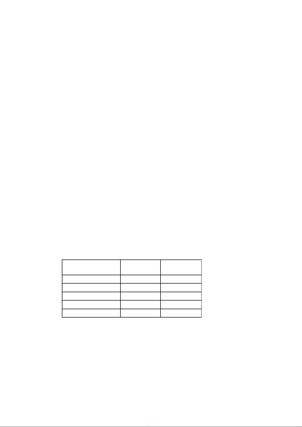
The next figure contains maps obtained using the ABOS and Kriging method. In both cases
negative values were substituted with zero values. According to the opinion of many SurGe
users, “pits” and “circular” contours in the surface generated by the Kriging method are un-
desirable.
interpolation method exceeding the
minimal value
exceeding the
maximal value
Kriging -18,8455 -4,4299
Radial basis functions -18,8455 -4,4299
Minimum curvature -46,4989 +0,7771
ABOS, q=0,5 -24,7731 +1,9323
ABOS, q=3,0 -16,6539 +1,8871
64
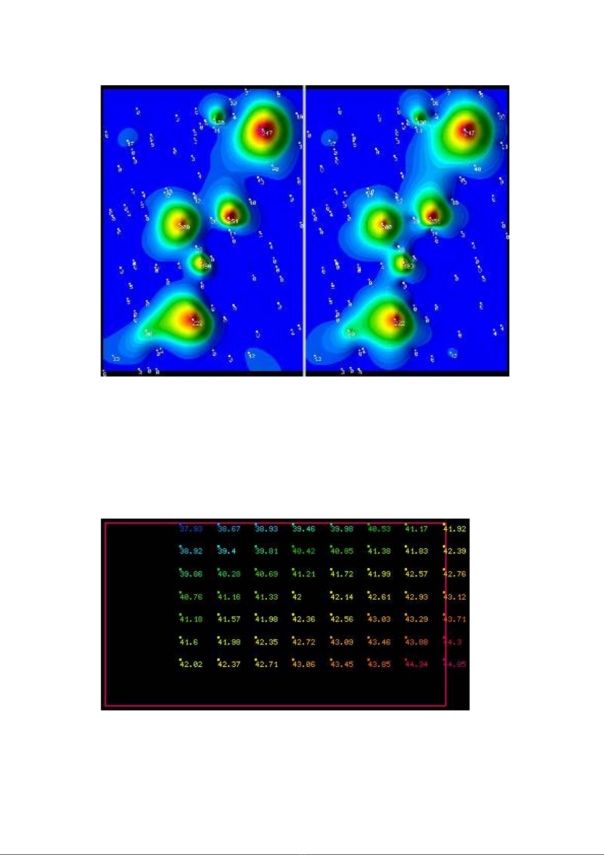
Fig. 5.1: Map of sulphate concentration created using the ABOS and Kriging method.
5.2 Extrapolation outside the XYZ points domain
The extrapolation properties of the ABOS method was examined in paragraph 2.4.3 Con-
servation of an extrapolation trend. Let us note that we only examined the domain determ-
ined by points XYZ. In the next example (see figure 5.2a), aerodynamic resistance data
measured at a small part of a racing car body was interpreted to obtain results outside the
domain determined by points XYZ.
Fig. 5.2a: Aerodynamic resistance data measured at a small part of a racing car body.
As the picture indicates, the desired domain of the interpolation function set by the bound-
ary (red rectangle) exceeds the domain defined by the points XYZ. The boundary was set so
that the aerodynamic resistance could be estimated aside the data on the left and bottom.
65
The interpreter tested several interpolation methods available in the Surfer software but
without satisfactory result.
As explained in paragraph 4.2.3.10 Interpolation with a trend surface, SurGe implements a
special procedure enabling to conserve the extrapolation trend. This procedure was imple-
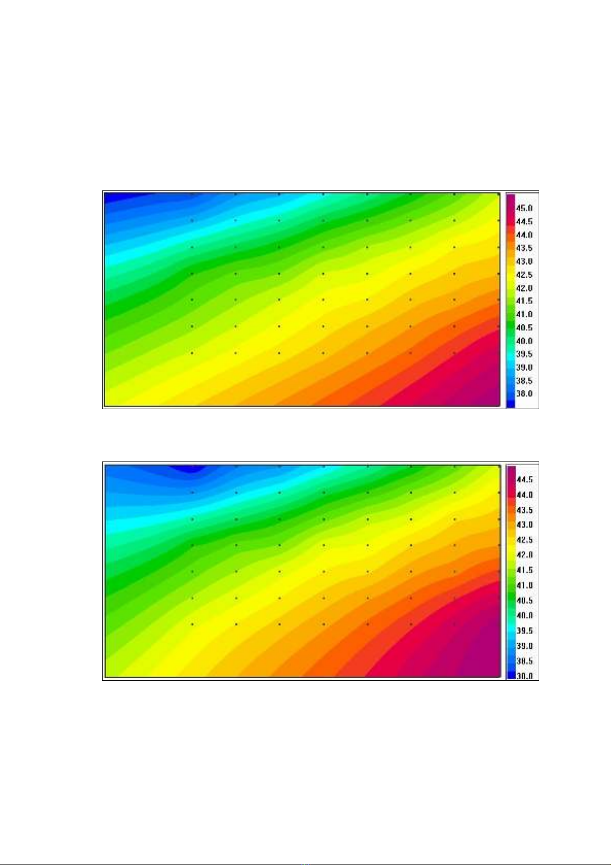
mented to the examined data with the result represented in figure 5.2.b. For comparison,
figures 5.2.c and 5.2.d contains results from the Kriging and Minimum curvature methods,
which were not accepted as satisfactory.
Fig. 5.2.b: Aerodynamic resistance data interpolated by SurGe.
Fig. 5.2.c: Aerodynamic resistance data interpolated by the Kriging method.
66
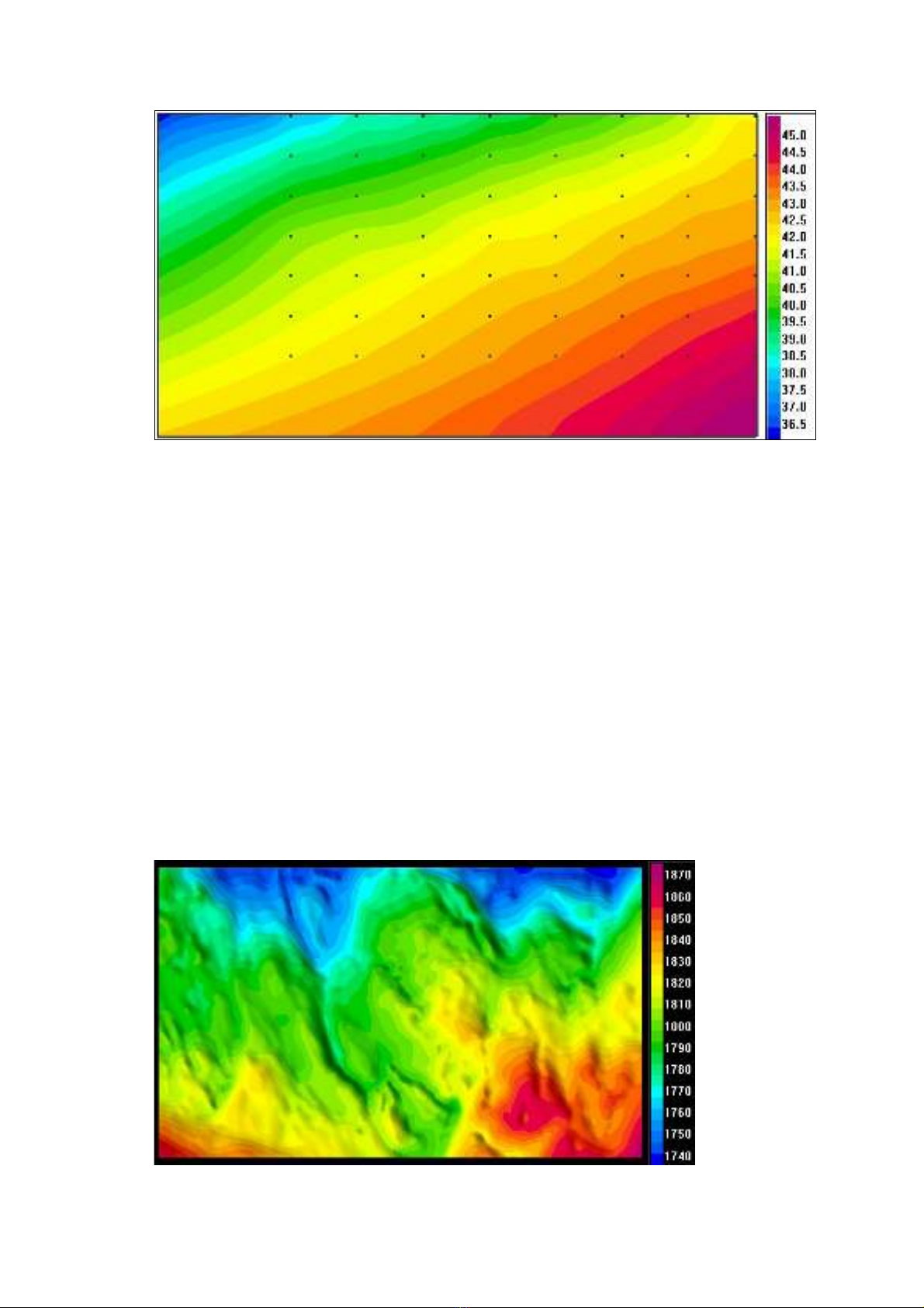
Fig. 5.2.d: Aerodynamic resistance data interpolated by the Minimum curvature method.
5.3 Seismic measurement
The processing of seismic data is one of the most significant tasks for geologists if they
have to create a geological map of some underground rock structure. The typical results of
seismic measurement are times at which reflected sound waves return from a certain bound-
ary between different types of rock. These times are, of course, measured from some datum
level and they are usually recorded using a dense mesh covering the area of interest with a
typical number of nodes between 10000 and 100000.
Because the homogeneity of covering rocks cannot be assumed and the speed of sound
waves in covering rocks is unknown or known only approximately, the measurement must
be supported by precise depth values usually measured at exploration wells. In general, the
interpreter has to work with two sets of data – the first one is the dense mesh of reflection
times and the second one is the measurement of rock structure depth at wells. Let us note
that the number of wells is usually small in comparison to the number of points at which the
reflection time is measured.
To demonstrate the interpretation of seismic measurement we will use the data set SEIS-
M1.DTc containing reflection times – the corresponding grid is shown in the next figure.
Fig. 5.3.a: Grid of reflection times created from the SEISM1.DTc data set.
67

The file SEISM1.DTc contains reflection times in the range from 1736 to 1875 seconds at
25853 points. It is obvious that the lower the value of reflection time, the higher the position
of the rock structure boundary.
The depth of the rock structure was also measured at 14 wells and the results were stored in
the file containing the second data set SEISM1.DTa – see the next list of the file content.
1225.976 2339.511 -2246 W-01
837.871 2270.595 -2250 W-02
428.004 2118.255 -2271 W-03
859.634 1878.863 -2272 W-04
181.357 1519.776 -2292 W-05
1940.525 2187.171 -2277 W-06
2738.498 2292.358 -2255 W-07
2981.517 2375.783 -2238 W-08
3344.232 935.805 -2338 W-09
2121.882 812.481 -2317 W-10
493.292 500.547 -2309 W-11
1519.776 1733.777 -2267 W-12
3663.421 2143.645 -2264 W-13
2999.652 2172.662 -2252 W-14
As follows from the list, the range of depths is -2338 to -2238 meters. As a rule, the depth
of a geological structure has a negative value measured from some datum plane (for ex-
ample sea-level).
The standard procedure of seismic data processing is the following:
1. The map of reflection times is created.
2. For all wells the sound speed is calculated from known structure depth and reflec-
tion time at the well.
3. The velocities known at well positions are used for the creation of the so-called ve-
locity map.
4. The velocity map is multiplied by the map of reflection times and thus the map of
depths is obtained.
The SURGEF offers another solution: to create a depth map directly from the structure
depths at wells using the reflection time grid as an external grid. This means that the grid
containing the map of reflection times SEISM1f.GRc is copied (renamed) into the file
SEISM1f.GRa and this grid is read at the beginning of the interpolation process. It may
seem to be strange especially if we realize that the reflection times are positive values while
the structure depths are negative. Let us have a closer look at the procedures performed by
SURGEF.
Firstly, SURGEF is run for the data set SEISM1.DTa and it is instructed to read the external
grid SEISM1f.GRa (which is a copy of SEISM1f.GRc and represents the map of reflection
times) by answering Y to the prompt:
READ FILE .GRD? (Y/N) [N] Y
Then SURGEF changes this grid using the linear transformation
a⋅Pi , j bPi , j
, where
the constants a and b minimize the term
∑
i=1
n
a⋅fXi, Y ib−DZi2
, as described in sec-
tion 2.2.8 Iteration cycle.
In this case the constant a was computed as the negative number -1.160139 and together
with b (-217.38) changed the grid so that the sum of squared differences between the new
68


![Bài giảng Tin học đại cương Trường Đại học Lâm Nghiệp [Năm mới nhất]](https://cdn.tailieu.vn/images/document/thumbnail/2026/20260514/hoahongxanh0906/135x160/85781779160272.jpg)
![Giáo trình Cấu trúc dữ liệu và giải thuật - TS. Đào Thị Hường [Mới nhất]](https://cdn.tailieu.vn/images/document/thumbnail/2026/20260514/hoahongxanh0906/135x160/49281779160273.jpg)


![Câu hỏi ôn tập Đồ hoạ máy tính [năm/khóa/chương trình]](https://cdn.tailieu.vn/images/document/thumbnail/2026/20260514/hoahongxanh0906/135x160/48771779155952.jpg)


%20--%3e%3cdefs%3e%3cstyle%3e%20.st0%20{%20fill:%20%23fff;%20}%20.st1%20{%20fill:%20%237800fa;%20}%20%3c/style%3e%3c/defs%3e%3cpath%20class='st1'%20d='M117.78,12.18H43.11c2.9,3.47,4.65,7.94,4.65,12.82,0,5.6-2.3,10.66-6.01,14.29h76.02l7.22-13.56-7.22-13.56Z'/%3e%3cg%3e%3cpath%20class='st0'%20d='M53.58,26.17h-.59v-1.46h.59v-4.96h2.83c1.78,0,2.67.94,2.67,2.82v5.76c0,1.87-.89,2.81-2.67,2.81h-2.83v-4.96ZM55.36,21.37v3.34h1.1v1.46h-1.1v3.34h1.01c.61,0,.91-.37.91-1.1v-5.93c0-.74-.3-1.1-.91-1.1h-1.01Z'/%3e%3cpath%20class='st0'%20d='M65.99,31.14h-1.8l-.31-2.07h-2.19l-.31,2.07h-1.64l1.82-11.39h2.62l1.82,11.39ZM65.28,18.04c-.25.46-.51.77-.75.94-.21.15-.47.22-.79.22-.26,0-.57-.07-.92-.22l-.38-.15c-.14-.05-.26-.07-.37-.07-.3,0-.53.18-.71.54l-.91-.68c.25-.46.51-.77.75-.94.21-.14.48-.21.79-.21.26,0,.57.07.92.21l.38.15c.14.05.26.07.37.07.3,0,.53-.18.71-.54l.91.68ZM61.91,27.52h1.73l-.87-5.76-.87,5.76Z'/%3e%3cpath%20class='st0'%20d='M74.53,26.89v1.52c0,1.91-.89,2.86-2.67,2.86s-2.67-.95-2.67-2.86v-5.93c0-1.91.89-2.86,2.67-2.86s2.67.95,2.67,2.86v1.11h-1.69v-1.22c0-.75-.31-1.12-.93-1.12s-.93.37-.93,1.12v6.15c0,.74.31,1.11.93,1.11s.93-.37.93-1.11v-1.63h1.69Z'/%3e%3cpath%20class='st0'%20d='M81.4,31.14h-1.8l-.31-2.07h-2.19l-.31,2.07h-1.64l1.82-11.39h2.62l1.82,11.39ZM75.9,19.2l1.52-1.91h1.71l1.51,1.91h-1.61l-.76-.95-.75.95h-1.61ZM77.32,27.52h1.73l-.87-5.76-.87,5.76ZM83.1,15.99l-1.76,1.91h-1.26l1.17-1.91h1.86Z'/%3e%3cpath%20class='st0'%20d='M84.86,19.75c1.78,0,2.67.94,2.67,2.82v1.48c0,1.87-.89,2.81-2.67,2.81h-.85v4.28h-1.79v-11.39h2.64ZM84.01,21.37v3.86h.85c.58,0,.87-.36.87-1.08v-1.71c0-.71-.29-1.07-.87-1.07h-.85Z'/%3e%3cpath%20class='st0'%20d='M93.51,19.75c1.78,0,2.67.94,2.67,2.82v1.48c0,1.87-.89,2.81-2.67,2.81h-.85v4.28h-1.79v-11.39h2.64ZM92.66,21.37v3.86h.85c.58,0,.87-.36.87-1.08v-1.71c0-.71-.29-1.07-.87-1.07h-.85Z'/%3e%3cpath%20class='st0'%20d='M98.8,31.14h-1.79v-11.39h1.79v4.88h2.03v-4.88h1.83v11.39h-1.83v-4.88h-2.03v4.88Z'/%3e%3cpath%20class='st0'%20d='M105.36,24.55h2.46v1.62h-2.46v3.34h3.09v1.63h-4.88v-11.39h4.88v1.63h-3.09v3.18ZM108.17,17.29l-1.76,1.91h-1.26l1.17-1.91h1.86Z'/%3e%3cpath%20class='st0'%20d='M112.2,19.75c1.78,0,2.67.94,2.67,2.82v1.48c0,1.87-.89,2.81-2.67,2.81h-.85v4.28h-1.79v-11.39h2.64ZM111.35,21.37v3.86h.85c.58,0,.87-.36.87-1.08v-1.71c0-.71-.29-1.07-.87-1.07h-.85Z'/%3e%3c/g%3e%3ccircle%20class='st1'%20cx='25'%20cy='25'%20r='20'/%3e%3cpath%20class='st0'%20d='M32.78,19.27c2.92,0,4.43,2.55,5.28,5.33l.71,2.17c.14.38-.33.75-.71.75h-5.61c.19-.33.24-.71.09-1.08l-.75-2.45c-.43-1.32-.99-2.64-1.79-3.77.75-.57,1.65-.94,2.78-.94h0ZM25,18.38c3.25,0,4.9,2.78,5.89,5.89l.76,2.45c.14.42-.33.8-.8.8h-11.69c-.42,0-.94-.38-.8-.8l.75-2.45c.99-3.11,2.64-5.89,5.89-5.89h0ZM25,11.35c1.74,0,3.11,1.37,3.11,3.11s-1.37,3.11-3.11,3.11-3.11-1.41-3.11-3.11,1.41-3.11,3.11-3.11h0ZM17.27,19.27c1.08,0,1.98.38,2.73.94-.8,1.13-1.37,2.45-1.74,3.77l-.8,2.45c-.14.38-.05.75.09,1.08h-5.56c-.42,0-.9-.38-.75-.75l.71-2.17c.9-2.78,2.41-5.33,5.33-5.33h0ZM17.27,12.91c1.51,0,2.78,1.27,2.78,2.83s-1.27,2.83-2.78,2.83-2.83-1.27-2.83-2.83,1.27-2.83,2.83-2.83h0ZM32.78,12.91c1.56,0,2.78,1.27,2.78,2.83s-1.23,2.83-2.78,2.83-2.83-1.27-2.83-2.83,1.27-2.83,2.83-2.83h0ZM27.07,28.56v.09c0,.57-.24,1.08-.61,1.46h0v.05c-.38.33-.9.57-1.46.57s-1.08-.24-1.46-.61h0c-.38-.38-.61-.9-.61-1.46v-.09h1.41v.09c0,.19.05.38.19.47v.05c.09.09.28.19.47.19s.38-.09.47-.19v-.05c.14-.09.24-.28.24-.47t-.05-.09h1.41ZM30.99,28.56v.09c0,1.65-.66,3.16-1.74,4.24-1.08,1.08-2.59,1.79-4.24,1.79s-3.16-.71-4.24-1.79l-.05-.05c-1.04-1.08-1.7-2.55-1.7-4.2v-.09h1.41v.09c0,1.27.47,2.4,1.27,3.25h.05c.85.85,1.98,1.37,3.25,1.37s2.4-.52,3.25-1.37c.85-.8,1.37-1.98,1.37-3.25v-.09h1.37ZM34.99,28.56v.09c0,2.78-1.13,5.28-2.92,7.07-1.79,1.79-4.29,2.92-7.07,2.92s-5.23-1.13-7.07-2.92c-1.79-1.79-2.92-4.29-2.92-7.07v-.09h1.41v.09c0,2.4.94,4.53,2.5,6.08,1.56,1.56,3.72,2.5,6.08,2.5s4.52-.94,6.08-2.5c1.56-1.56,2.5-3.68,2.5-6.08v-.09h1.41Z'/%3e%3c/svg%3e)