For simplicity, in the example we have assumed that a new map is created at the end of every
step. This is certainly a possibility, but it is not necessarily the best option. Later in this book, we will
discuss data modeling and how to optimize the sequence of operations. In particular, Chapters 8
and 9 cover spatial operators and functions that make it possible to cluster some of the steps in the
example into single queries, making the process much simpler and more efficient.
Storing Spatial Data in a Database
Looking at vector data, we usually distinguish between the following:
•Points (for example, the plots for sale in Figure 1-1), whose spatial description requires only
x,y coordinates (or x,y,z if 3D is considered)
•Lines (for example, roads), whose spatial description requires a start coordinate, an end
coordinate, and a certain number of intermediate coordinates
•Polygons (for example, a residential area), which are described by closed lines
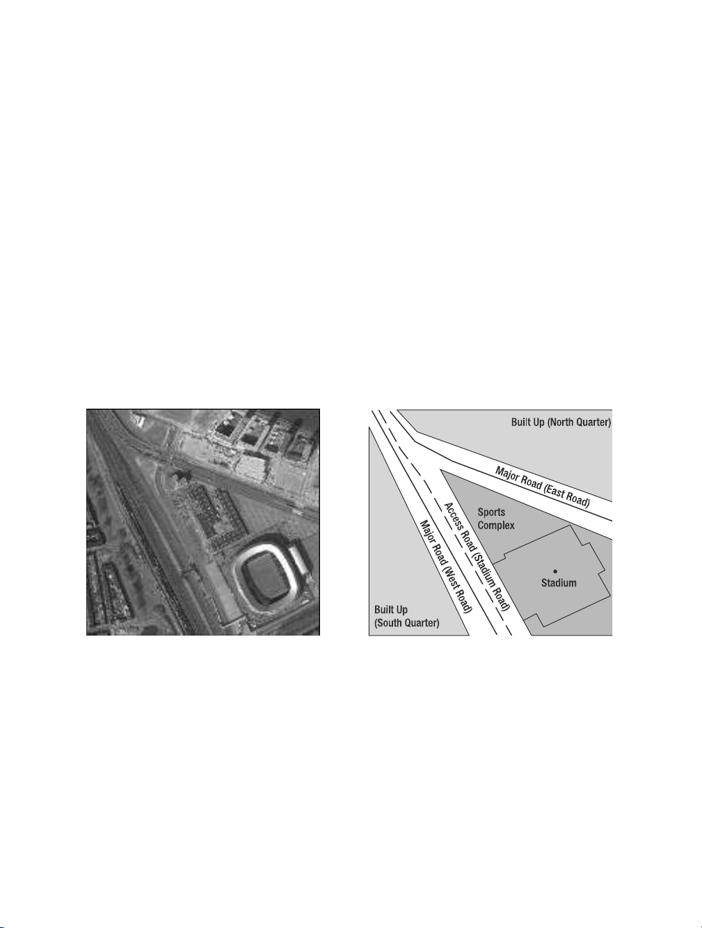
Figure 1-2 shows an example containing point, line, and polygon data. The figure corresponds
to a small portion of the area used in the previous site selection example. The vector representation,
here simplified for convenience, shows a point (the stadium), three lines (the roads), and four poly-
gons (the built-up areas, clipped at the picture borders, and the sports complex).
Figure 1-2. Vector representation of the spatial objects in the picture
The vector data in Figure 1-2 could be stored in one or multiple tables. The most natural way of
looking at this data is to identify data layers—sets of data that share common attributes—that become
data tables. Most spatial databases use a special data type to store spatial data in a database. Let’s
refer to this type as the geometry. Users can add columns of type geometry to a database table in
order to store spatial objects.
CHAPTER 1 ■SPATIAL INFORMATION MANAGEMENT 11

In this case, the choice of tables would be rather simple with three main data layers present:
“Road infrastructures,” “Land use,” and “Points of interest.” These three layers contain objects that
share common attributes, as shown in the three tables later in this section. The same objects could
have been aggregated into different data layers, if desired. For instance, we could have stored major
and minor roads in different tables, or we could have put roads and land use in the same table. The
latter would make sense if the only attributes of relevance for roads and land-use areas were the same,
for instance, the province name and the city name. It is also worth stressing that every geometry
column can contain any mix of valid spatial object (points, lines, polygons) and also that every table
can contain one or more geometry columns.
Structuring spatial data into tables and defining the right table structure are the first logical
activities of any spatial analysis. Fortunately, in most cases there is an intuitive correspondence
between the data and the table structure used to store them. However, in several cases you may find
that the spatial database design can be a complex activity. Proper designs may facilitate analysis
enormously, while poor data structures may make the analysis complex and slow. These issues are
addressed in various places in the book but in particular in Chapter 3.
Table 1-2 shows the road infrastructure table of Figure 1-2. This table contains three records
corresponding to the east road, the west road, and the stadium road. All of them are represented as
lines using the geometry type. Each road is described by three types of attributes: the road type (one
column containing either “major,” “local,” or “access” road), the road name (a column containing
the name of the road as used in postal addresses), and the area attributes (two columns containing
the name of the province and city where the road is located).
Table 1-2. Road Infrastructure Table
ID Province City Road Name Road Type Road Geometry
1 Province name City name West road Major road
2 Province name City name East road Major road
3 Province name City name Stadium road Access road
Table 1-3 shows the land-use table. It contains three records corresponding to the north quarter,
the south quarter, and the sports complex. In this case, all spatial objects are polygons. Each object
has three types of attributes: the surface of the area (in square meters), the name of the area, and
the area location (province and city names).
CHAPTER 1 ■SPATIAL INFORMATION MANAGEMENT12

Table 1-3. Land Use Table
Surface (Square
ID Province City Area Name Meters) Area Geometry
1 Province name City name North quarter 10,000
2 Province name City name South quarter 24,000
3 Province name City name Sports complex 4,000
Table 1-4 shows the points of interest (POI) in the area. It contains two records: a point (in this
case, the center of the stadium complex) and a polygon (in this case, the contour of the stadium
complex). Attributes include the type of POI from a classification list, the POI name, and the
province and city where they are located.
Table 1-4. Points of Interest Table
ID Province City POI Name Type of POI POI Geometry
1 Province name City name Olympic Sports
stadium location
2 Province name City name Olympic Sports
stadium infrastructure
In the Table 1-4, we use two records to describe the same object with two different geometries.
Another option for storing the same information is presented in Table 1-5, where we use two columns of
type geometry to store two different spatial features of the same object. The first geometry column
stores the POI location, while the second stores the outline of the complex. Under the assumption
that all other nonspatial attributes are the same, Table 1-5 is a more efficient use of table space than
Table 1-4.
Table 1-5. Points of Interest Table: Two Geometry Columns
Location (POI) Infrastructure
ID Province City POI Name Geometry Geometry
1 Province name City name Olympic
stadium
CHAPTER 1 ■SPATIAL INFORMATION MANAGEMENT 13

The objects in the preceding tables are represented with different line styles and fill patterns.
This information is added for clarity, but in practice it is not stored in the geometry object. In Oracle
Spatial, the geometry data are physically stored in a specific way (which we will describe in Chapters 3
and 4) that does not have a direct relationship to the visual representation of the data. Chapter 12,
which describes the Oracle Application Server MapViewer, shows how symbology and styling rules
are used for rendering geometry instances in Oracle.
Geometry models in the SQL/MM and Open Geospatial (OGC) specifications describe in detail
the technical features of the geometry type and how points, lines, and polygons are modeled using
this type.
Spatial Analysis
Once data is stored in the appropriate form in a database, spatial analysis makes it possible to
derive meaningful information from it. Let’s return to the site selection example and look again at
the three types of spatial operations that we used:
•Select, used in the following:
• Step 1 (to select areas where the attribute was a certain value)
• Step 2 (to select large sites from the sites for sale)
• Step 4 (to select major roads from the road network)
•Overlay, used in the following:
• Step 5 (large sites in commercial areas)
• Step 7 (sites away from risk areas)
• Step 8 (sites within highly accessible areas)
•Buffer, used in the following:
• Step 3 (areas subject to flood risk)
• Step 6 (high accessibility areas)
Returning to our example, assuming we have the data stored in a database, we can use the follow-
ing eight pseudo-SQL statements to perform the eight operations listed previously. Please note that for
the sake of the example, we have assumed certain table structures and column names. For instance, we
have assumed that M1 contains the columns LAND_USE_TYPE,AREA_NAME, and AREA_GEOMETRY.
1. Use
SELECT AREA_NAME, AREA_GEOMETRY
FROM M1
WHERE LAND_USE_TYPE='COMMERCIAL'
to identify available plots of land for which a construction permit can be obtained for
a shopping mall.
2. Use
SELECT SITE_NAME, SITE_GEOMETRY
FROM M2
WHERE SITE_PLOT_AREA > <some value>
to identify available sites whose size is larger than a certain value.
CHAPTER 1 ■SPATIAL INFORMATION MANAGEMENT14

3. Use
SELECT BUFFER(RIVER_GEOMETRY, 1, 'unit=km')
FROM M3
WHERE RIVER_NAME= <river_in_question>
to create a buffer of 1 kilometer around the named river.
4. Use
SELECT ROAD_NAME, ROAD_GEOMETRY
FROM M4
WHERE ROAD_TYPE='MAJOR ROAD'
to identify major roads.
5. Use the contains operator to identify the sites selected in step 2 that are within areas
selected in step 1. You could also achieve this in one step starting directly from M1 and M2:
SELECT SITE_NAME, SITE_GEOMETRY
FROM M2 S, M1 L
WHERE CONTAINS(L.AREA_GEOMETRY, S.SITE_GEOMETRY)='TRUE'
AND L.LAND_USE_TYPE= 'COMMERCIAL'
AND S.SITE_AREA > <some value>;.
6. As in step 3, use the buffer function to create a buffer of a certain size around the major
roads.
7. Use contains to identify sites selected in step 5 that are outside the flood-prone areas identi-
fied in step 3.
8. Use contains to identify safe sites selected in step 7 that are within the zones of easy accessi-
bility created in step 6.
Oracle Spatial contains a much wider spectrum of SQL operators and functions (see Chapters 8
and 9). As you might also suspect, the preceding list of steps and choice of operators is not optimal.
By redesigning the query structures, changing operators, and nesting queries, it is possible to drasti-
cally reduce the number of intermediate tables and the queries. M11, for instance, could be created
starting from M9 and M3 directly by using the nearest-neighbor and distance operations together.
They would select the nearest neighbor and verify whether the distance is larger than a certain value.
Benefits of Oracle Spatial
The functionality described in the previous section has been the main bread and butter for GIS for
decades. In the past five to ten years, database vendors such as Oracle have also moved into this
space. Specifically, Oracle introduced the Oracle Spatial suite of technology to support spatial pro-
cessing inside an Oracle database.
Since GIS have been around for several years, you may wonder why Oracle has introduced yet
another tool for carrying out the same operations. After all, we can already do spatial analysis with
existing tools.
The answer lies in the evolution of spatial information technology and in the role of spatial
data in mainstream IT solutions. GIS have extensive capabilities for spatial analysis, but they have
historically developed as stand-alone information systems. Most systems still employ some form of
dual architecture, with some data storage dedicated to spatial objects (usually based on proprietary
formats) and some for their attributes (usually a database). This choice was legitimate when main-
stream databases were unable to efficiently handle the spatial data. However, it has resulted in the
proliferation of proprietary data formats that are so common in the spatial information industry.
CHAPTER 1 ■SPATIAL INFORMATION MANAGEMENT 15


![Tập bài giảng Thiết kế đa phương tiện (Nghề: Công nghệ thông tin) - Trường Cao đẳng Nông nghiệp Thanh Hóa [Mới nhất]](https://cdn.tailieu.vn/images/document/thumbnail/2026/20260423/songngu_011/135x160/79441777364094.jpg)


