REGULAR ARTICLE
On the use of the BMC to resolve Bayesian inference
with nuisance parameters
Edwin Privas
*
, Cyrille De Saint Jean, and Gilles Noguere
CEA, DEN, Cadarache, 13108 Saint Paul les Durance, France
Received: 31 October 2017 / Received in nal form: 23 January 2018 / Accepted: 7 June 2018
Abstract. Nuclear data are widely used in many research elds. In particular, neutron-induced reaction cross
sections play a major role in safety and criticality assessment of nuclear technology for existing power reactors
and future nuclear systems as in Generation IV. Because both stochastic and deterministic codes are becoming
very efcient and accurate with limited bias, nuclear data remain the main uncertainty sources. A worldwide
effort is done to make improvement on nuclear data knowledge thanks to new experiments and new adjustment
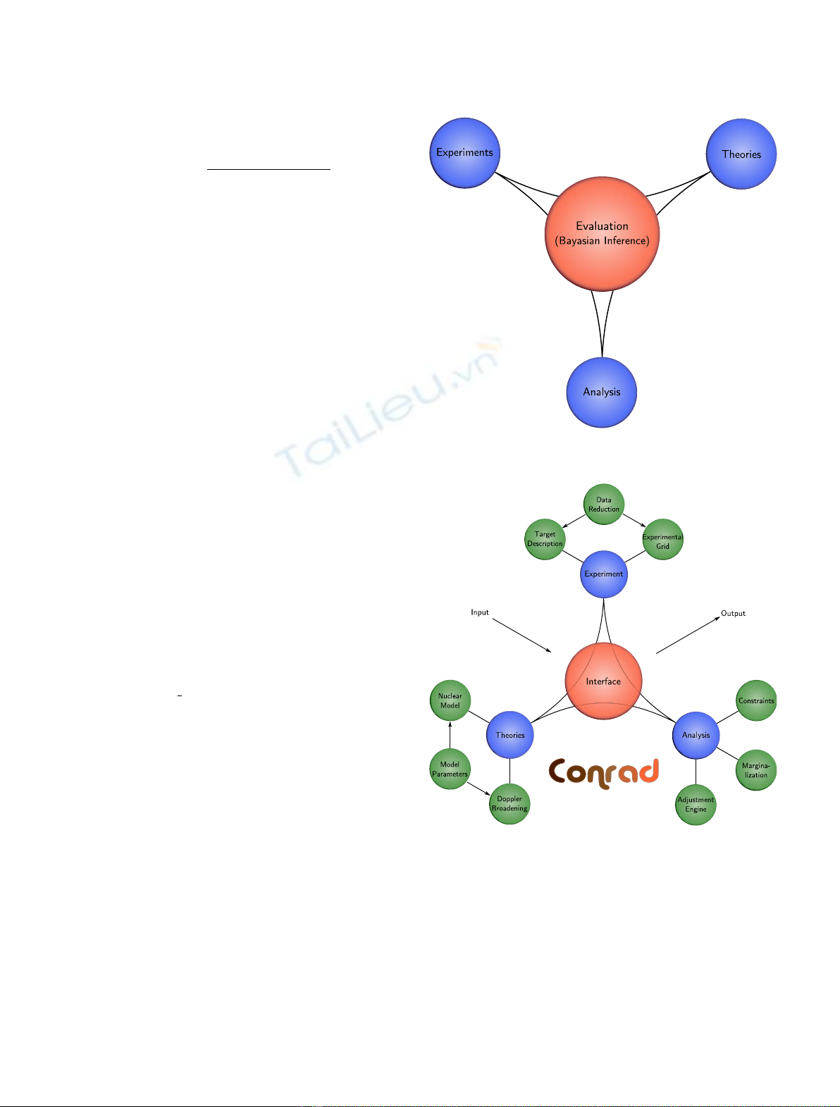
methods in the evaluation processes. This paper gives an overview of the evaluation processes used for nuclear
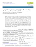
data at CEA. After giving Bayesian inference and associated methods used in the CONRAD code [P. Archier
et al., Nucl. Data Sheets 118, 488 (2014)], a focus on systematic uncertainties will be given. This last can be deal
by using marginalization methods during the analysis of differential measurements as well as integral
experiments. They have to be taken into account properly in order to give well-estimated uncertainties on
adjusted model parameters or multigroup cross sections. In order to give a reference method, a new stochastic
approach is presented, enabling marginalization of nuisance parameters (background, normalization...). It can
be seen as a validation tool, but also as a general framework that can be used with any given distribution. An
analytic example based on a ctitious experiment is presented to show the good ad-equations between the
stochastic and deterministic methods. Advantages of such stochastic method are meanwhile moderated by the
time required, limiting its application for large evaluation cases. Faster calculation can be foreseen with nuclear
model implemented in the CONRAD code or using bias technique. The paper ends with perspectives about new
problematic and time optimization.
1 Introduction
Nuclear data continue to play a key role, as well as
numerical methods and the associated calculation schemes,
in reactor design, fuel cycle management and safety
calculations. Due to the intensive use of Monte-Carlo
tools in order to reduce numerical biases, the nal accuracy
of neutronic calculations depends increasingly on the
quality of nuclear data used. The knowledge of neutron
induced cross section in the 0 eV and 20 MeV energy range
is traduced by the uncertainty levels. This paper focuses
on the neutron induced cross sections uncertainties
evaluation. The latter is evaluated by using experimental
data either microscopic or integral, and associated
uncertainties. It is very common to take into account the
statistical part of the uncertainty using the Bayesian
inference. However, systematic uncertainties are not often
taken into account either because of the lack of information
from the experiment or the lack of description by the
evaluators.
Arst part presents the ingredients needed in the
evaluation of nuclear data: theoretical models, microscopic
and integral measurements. A second part is devoted to the
presentation of a general mathematical framework related to
Bayesian parameters estimations. Two approaches are then
studied: a deterministic and analytic resolution of the
Bayesian inference and a method using Monte-Carlo
sampling. The next part deals with systematic uncertainties.
More precisely, a new method has been developed to solve the
Bayesian inference using only Monte-Carlo integration. A
nal part gives a ctitious example on the
235
U total cross
section and comparison between the different methods.
2 Nuclear data evaluation
2.1 Bayesian inference
Let y¼~
yiði¼1...NyÞdenote some experimentally mea-
sured variables, and let xdenote the parameters dening the
model used to simulate theoretically these variables and tis
the associated calculated values to be compared with y.
Using Bayestheorem [1] and especially its generalization to
*e-mail: edwin.privas@gmail.com
EPJ Nuclear Sci. Technol. 4, 36 (2018)
©E. Privas et al., published by EDP Sciences, 2018
https://doi.org/10.1051/epjn/2018042
Nuclear
Sciences
& Technologies
Available online at:
https://www.epj-n.org
This is an Open Access article distributed under the terms of the Creative Commons Attribution License (http://creativecommons.org/licenses/by/4.0),
which permits unrestricted use, distribution, and reproduction in any medium, provided the original work is properly cited.
continuous variables, one can obtain the well known relation
between conditional probability density functions (written p
(.)) when the analysis of a new dataset yis performed:
pðxjy;UÞ¼ pðxjUÞpðyjx;UÞ
dxpðxjUÞpðyjx;UÞ;ð1Þ
where Urepresents the backgroundor priorinformation
from which the prior knowledge of xis assumed. Uis
supposed independent of y. In this framework, the
denominator is just a normalization constant.
The formal rule [2] used to take into account
information coming from new analyzed experiments is:
posteriorpriorlikelihood:ð2Þ
The idea behind tting procedures is to nd an
estimation of at least the rst two moments of the
posterior density probability of a set of parameters x,
knowing an a priori information (or rst guess) and a
likelihood which gives the probability density function of
observing a data set knowing x.
Algorithms described in this section are summarized
and detailed description can be found in paper linked to the
CONRAD code in which they are implemented [3]. A
general overview of the evaluation process and the conrad
code is given in Figures 1 and 2.
2.2 Deterministic theory
To obtain an equation to be solved, one has to make
some assumptions on the prior probability distribution
involved.
Given a covariance matrix and mean values, the choice of
a multivariate joint normal for the probability density pðxjUÞ
and for the likelihood is maximizing the entropy [4]. Adding
Bayestheorem, equation (1) canbewrittenasfollow:
pðxjy;UÞe1
2½ðxxmÞTM1
xðxxmÞþðytÞTM1
yðytÞ;ð3Þ
where x
m
(expectation) and M
x
(covariance matrix) are
prior information on x,yan experimental set and M
y
the
associated covariance matrix. trepresents the theoretical
model predictions.
The Laplace approximation is also made. It enables
to approximate the posterior distribution by a multivariate
normal distribution with the same maximum and curvature
of the rightside of equation (3). Then, it can be demonstrated
that both the posterior expectation and the covariances can
be calculated by nding the minimum of the following cost
function (Generalized Least Square):
x2
GLS ¼ðxxmÞTM1
xðxxmÞþðytÞTM1
yðytÞ:ð4Þ
To take into account non-linear effects and ensure a
proper convergence of the algorithm, a GaussNewton
iterative solution can be used [5].
Thus, from a mathematical point of view, the
evaluation of parameters through a GLS procedure suffers
from the Gaussian choice as guessed distribution for the
prior and the likelihood, the use of Laplace approximation,
the linearization around the prior for Gauss-Newton
algorithm and at last a 2nd order terms neglected in the
GaussNewton iterative procedure.
2.3 Bayesian Monte-Carlo
Bayesian Monte-Carlo (BMC) methods are natural
solutions for Bayesian inference problems. They avoid
approximations and propose alternatives in probability
Fig. 1. General overview of the evaluation process.
Fig. 2. General overview of the CONRAD code.
2 E. Privas et al.: EPJ Nuclear Sci. Technol. 4, 36 (2018)
density distribution choice for priors and likelihoods. This
paper exposes the use of BMC in the whole energy range
from thermal, resonance to continuum range.
BMC can be seen as a reference calculation tool to
validate the GLS calculations and approximations. In
addition, it allows to test probability density distributions
effects and to nd higher distribution moments with no
approximations.
2.3.1 Classical Bayesian Monte-Carlo
The main idea of classicalBMC is the use of Monte-Carlo
techniques to calculate integrals. For any function fof
random variable set x, any integral can be calculated by a
Monte-Carlo sampling:
ZpðxÞfðxÞdx¼lim
n
!
1
nX
n
k¼1
fðxkÞ
!
;ð5Þ
where p(x) is a probability density function. One can thus
estimate any moments of the probability function p(x). By
denition, the mean value is given by:
x¼ZxpðxÞdx:ð6Þ
Application of these simple features to Bayesian inference
analysis gives for posterior distributionsexpectation
values:
x¼ZxpðxjUÞpðyjx;UÞ
ZpðxjUÞpðyjx;UÞdx
dx:ð7Þ
The proposed algorithm to nd out the rst two
moments of the posterior distribution is to sample the prior
probability distribution function pðxjUÞNxtimes and for
each x
k
realization evaluate the likelihood:
Lk¼pðykjxk;UÞ:ð8Þ
Finally, the posterior expectation and covariance is
given by the following equation:
xiNx¼X
Nx
k¼1
xi;kLk
X
Nx
k¼1
Lk
;ð9Þ
xi;xjNx¼X
Nx
k¼1
xi;kxj;kLk
X
Nx
k¼1
Lk
xiNxxjNx:ð10Þ
The choice of the prior distribution depends on what
kind of analysis is done. If no prior information is given, a
non-informative prior could be chosen (uniform distribu-
tion). On the contrary, for an update of a given parameters
set, the prior is related to a previous analysis with a known
probability distribution function.
The use of Lkweights indicates clearly the major
drawbacks of this classical BMC method: if the prior is far
from high likelihood values and/or by nature Lkvalues are
small (because of the number of experimental points for
example), then the algorithm will have difculties to
converge.
Thus, the main issue is that the covered phase space of
sampling is not favorable to convergence. In practice a trial
function close to the posterior distribution should be
chosen for sampling.
More details can be found in paper [6].
2.3.2 Importance sampling
As previously exposed, the estimation of the integral of f(x)
times a probability density function p(x) is not straightfor-
ward. Especially in this Bayesian inference case, sampling
the prior pðxjUÞdistribution, when it is far away from the
posterior distribution or when the likelihood weights are
difcult to evaluate properly, could be very expensive and
time consuming without any valuable estimation of posterior
distributions. The idea is then to sample in a different phase
space region by respecting statistics.
This trial probability density function p
trial
(x) can be
introduced by a trick as follow:
pðxÞ¼ pðxÞ
ptrialðxÞptrialðxÞ:ð11Þ
Thus, putting this expression in equation (5), one
obtains the following equation:
ZpðxÞfðxÞdx¼lim
n
!
1
nX
n
k¼1
pðxkÞ
ptrialðxkÞfðxkÞ
!
:ð12Þ
Then, sampling is done on the trial probability density
function p
trial
(x) getting a new set of {x
k
}. For each
realization x
k
, an evaluation of additional terms pðxÞ
pbiasðxÞ

is
necessary.
As a result, expectation and covariances are dened by:
xiNx¼X
Nx
k¼1
xi;khðxkÞLk
X
Nx
k¼1
hðxkÞLk
;ð13Þ
and
xi;xjNx¼X
Nx
k¼1
xi;kxj;khðxkÞLk
X
Nx
k¼1
hðxkÞLk
xiNxxjNx;ð14Þ
with hðxkÞ¼ pðxkjUÞ
ptrialðxkÞ.
The choice of trial functions is crucial and the closer
to the true solution p
trial
(x) is, the quicker the algorithm
will be. In this paper, a trialfunctionusedbydefault
E. Privas et al.: EPJ Nuclear Sci. Technol. 4, 36 (2018) 3
comes from the result of the generalized least square
(with additional standard deviation enhancement).
Many other solutions can be used depending on the
problem.
3 Systematic uncertainties treatment
3.1 Theory
Let recall some denitions and principles. First, it is
possible to link model parameters xand nuisance
parameters uwith conditional probability:
pðx;ujy;UÞ¼pðxju;y;UÞpðujy;UÞ;ð15Þ
with Uthe prior information on both model and nuisance
parameters. The latter is supposed independent to the
measurement. It means nuisance parameters are consid-
ered acting on experimental model. It induces
pðujy;UÞ¼pðujUÞ;giving the following equation:
pðx;ujy;UÞ¼pðxju;y;UÞpðujUÞ:ð16Þ
Moreover, evaluators are looking at the marginal
probability density pðx;ujy;UÞ;also written puðxjy;UÞ.It
is given by the integration of the probability
density function over marginal variables as follow:
puðxjy;UÞ¼Zpðx;ujy;UÞdu:ð17Þ
According to (16), the follow equation is obtained:
puðxjy;UÞ¼Zpðxju;y;UÞpðujUÞdu:ð18Þ
Then the Bayes theorem is used to calculate the rst
integral term of (18):
pðxju;y;UÞ¼ pðxjUÞpðyju;x;UÞ
ZpðxjUÞpðyju;x;UÞdx
:ð19Þ
This expression is right if both model and nuisance
parameters are supposed independent. According to (18)
and (19), the marginal probability density function of the a
posteriori model parameters is given by:
puðxjy;UÞ¼ZpðujUÞdupðxjUÞpðyju;x;UÞ
ZpðxjUÞpðyju;x;UÞdx
:ð20Þ
3.2 Deterministic resolution
The deterministic resolution is well described in Habert
thesis [7]. Several works have been rst performed in 1972
by H. Mitani and H. Kuroi [8,9] and later by Gandini [10]
giving a formalism to the multigroup adjustment and a
way to take into account the systematic uncertainties.
These were the rst attempts to consider the possible
presence of systematic errors in a data adjustment
process. Equations are not detailed here, only the idea
and the nal equation is provided.
Let Mstat
xbe the a posteriori covariance matrix
obtained after an adjustment. The a posteriori covariance
after marginalization Mmarg
xcan be found as
follow:
Mmarg
x¼Mstat
xþðGT
xGxÞ1GT
xGuMuGT
uGxðGT
xGxÞ1
ð21Þ
with G
x
sensitivities vector of the calculated model values
to the model parameters and G
u
sensitivities vector of the
calculated model values to the nuisance parameters.
Similar expressions have been given in reference [8,9]
where two terms appear: one for classical resolution and the
second for some added systematic uncertainties. ðGT
xGxÞis
a square matrix supposed reversal. It is often the case
when there are more experimental points than tted
parameters. If numeric issues appeared, it is mandatory to
nd another way, giving by a stochastic approach. Further
study should be undertaken to compare the deterministic
method proposed here and the one identied in Mitanis
papers in order to provide a more robust approach.
3.3 Semi-stochastic resolution
This method (written MC_Margi) is easy to understand
starting from the equation (20): nuisance parameters
are sampled according to a Gaussian distribution and
for each history, a deterministic resolution is done (GLS).
At the end of every simulation, parameters and covariances
are stored. When all the histories have been simulated, the
covariance total theorem gives the nal model parameters
covariance. The methods is not developed here but more
detailed can be found in papers [7,11].
3.4 BMC with systematic treatment
BMC method can deal with marginal parameters
without deterministic approach. This work has been
successfully implemented in the CONRAD code. One
wants to nd the posterior marginal probability function
dened in equation (20). It is similar to the case with no
nuisance parameters but with two integrals. Same
weighting principle can be applied by replacing the
likelihood term by a new weight wuðxjyÞdened by:
wuðxjyÞ¼ZpðujUÞpðyju;x;UÞ
ZpðxjUÞpðyju;x;UÞdx
du:ð22Þ
The very close similarities between the case with no
marginal parameter enabled a quick implementation
and understanding. Finally, the previous equation
gives:
puðxjy;UÞ¼pðxjUÞwuðxjyÞ:ð23Þ
4 E. Privas et al.: EPJ Nuclear Sci. Technol. 4, 36 (2018)
Both integrals can be solved using a Monte-Carlo
approach. The integral calculation of the equation (22) is
done as follow:
wuðxjyÞ¼ lim
nu
1
nuX
nu
l¼0
pðyjul;x;UÞ
ZpðxjUÞpðyjul;x;UÞdx
0
B
B
@1
C
C
A
:ð24Þ
The n
u
histories are calculated by sampling according to
pðujUÞ. The denominators integral of equation (24) is then
computed:
l1;nu;
ZpðxjUÞpðyjul;x;UÞdx¼lim
nx
1
nxX
nx
m¼0
pðyjul;xm;UÞ
!
:
ð25Þ
The n
x
histories are evaluated by sampling according to
pðxjUÞ. Mixing equations (24) and (25), the new weight
wuðxjyÞis given by:
lim
nu
1
nuX
nu
l¼0
pðyjul;x;UÞ
lim
nx
1
nxX
nx
m¼0
pðyjul;xm;UÞ
!
0
B
B
B
B
@
1
C
C
C
C
A
:ð26Þ
Let us consider N
x
is the number of history sampled
according the prior parameters and N
u
is the number of
history sampled according the marginal parameters. The
larger those number are, the more converge the results will
be. The previous equation can be numerically written with
no limits as follow:
wuðxjyÞ¼Nx
NuX
Nu
l¼0
pðyjul;x;UÞ
X
Nx
m¼0
pðyjul;xm;UÞ
:ð27Þ
In order to simplify the algorithm, N
u
and N
x
are
considered equal (introducing N as N=N
u
=N
x
). First, N
samples are drawn according to u
k
and x
k
. Equation (26)
can be simplied as follow:
wuðxjyÞ¼X
N
l¼0
pðyjul;x;UÞ
X
N
m¼0
pðyjul;xm;UÞ
:ð28Þ
In CONRAD, the N*Nvalues of the likelihood are
stored (i.e. ði;jÞ1;N2;pðyjuj;xi;UÞ. Those values
are required to perform statistical analysis at the end of
the simulation. The weight for an history k is then
calculated:
wuðxkjykÞ¼X
N
l¼0
pðykjul;xk;UÞ
X
N
m¼0
pðykjul;xm;UÞ
:ð29Þ
To get the posterior mean values and the posterior
correlation, one should apply the statistical denition and
get the two next equations:
xN¼1
NX
N
k¼0
xkX
N
l¼0
pðyjul;xk;UÞ
X
N
m¼0
pðyjul;xm;UÞ
;ð30Þ
Covðxi;xjÞN¼ðMxpost ÞNx
ij
¼xixjNxiNxjN;ð31Þ
with xixjNdened as the weighting mean of the two
parameters product:
xixjN¼1
NX
N
k¼1
xi;kxj;kwuðxkjykÞ:ð32Þ
4 Illustrative analysis on
238
U total cross
section
4.1 Study case
The selected study case is just an illustrative example
giving a very rst step towards the validation of the
method, its applicability and potential limitations. The
238
U total cross section is chosen and tted on the
unresolved resonance range, between 25 and 175 keV.
The theoretical cross section is calculated using the R mean
matrix model. The main sensitives parameters in this
energy range is the two rst strength functions S
l=0
and
S
l=1
.Tables 1 and 2give respectively the spin cong-
urations and the prior parameters governing the
total cross section. An initial relative uncertainties of
15% is taken into account with no correlations.
The experimental dataset used comes from the EXFOR
database [12]. A 1% arbitrary statistical uncertainty is
chosen.
Table 1.
238
U spin conguration considered for resonance
waves sand p.
ls J
p
g
J
onde
238
U(0
+
) 0 1/2 1/2
+
1s
1 1/2 1/2
3/2
12p
Table 2. Initial URR parameters with no correlation.
Parameters Values
S
0
1.290 10
4
± 10%
S
1
2.170 10
4
± 10%
E. Privas et al.: EPJ Nuclear Sci. Technol. 4, 36 (2018) 5