Cấu trúc sóng chức năng trong điện lý thuyết P8

Chia sẻ: Tien Van Van | Ngày: | Loại File: PDF | Số trang:18

Thêm vào BST

Báo xấu

107
lượt xem 8
download

Download Vui lòng tải xuống để xem tài liệu đầy đủ

Rainfall Attenuation Investigations on the attenuation caused by rain and other hydrometers and their effects on terrestrial communications started as early as in the 1940s. Subsequently, many theoretical and experimental results were obtained and used to predict the effects of interaction between hydrometers and microwave signals. The theories for the prediction of rain attenuation on microwave signals are well established and widely used by many researchers.

Chủ đề:

Bình luận(0) Đăng nhập để gửi bình luận!

Lưu

Nội dung Text: Cấu trúc sóng chức năng trong điện lý thuyết P8

Spheroidal Wave Functions in Electromagnetic Theory Le-Wei Li, Xiao-Kang Kang, Mook-Seng Leong Copyright  2002 John Wiley & Sons, Inc. ISBNs: 0-471-03170-4 (Hardback); 0-471-22157-0 (Electronic) 8 Analysis of Rainfall Attenuation Using Oblate Raindrops 8.1 INTRODUCTION 8.1.1 Rainfall Attenuation Investigations on the attenuation caused by rain and other hydrometers and their effects on terrestrial communications started as early as in the 1940s. Subsequently, many theoretical and experimental results were obtained and used to predict the effects of interaction between hydrometers and microwave signals. The theories for the prediction of rain attenuation on microwave signals are well established and widely used by many researchers. Concep- tually, the specific attenuation due to raindrops depends on both the total (extinction) cross section and the raindrop size distribution. In 1908, Mie [161] formulated and put forth the exact formulation for the calculation of the total cross section (TCS) of an isotropic, homogeneous di- electric sphere of arbitrary size. This is known as A&e theory. Later, Stratton [86] expanded the scattered fields into a series of spherical vector wave func- tions to calculate the TCS from which the attenuation can readily be obtained upon knowing the raindrop size distribution (DSD). In the work by Oslen et al. [162], an empirical relationship between the specific attenuation A and a rain rate R was proposed as A = aRb, where a = a(f) and b = b(f) are frequency-dependent parameters. Based on this formulation, a and b can readily be obtained via regression analysis for dif- ferent frequencies, a known drop size distribution and a given atmospheric temperature. The International Radio Consultative Committee (CCIR) (now known as CCITT) [163] recommended this relationship based on the Laws 227
228 ANALYSIS OF RAlNFALL ATTENUATlON USING OBLATE RAINDROPS and Parsons DSD [164] in the frequency range 1 to 1000 GHz. Using interpo lation, the unknowns a and b can be determined using the formula presented in the report. However, the Laws and Parsons DSD is only a representa- tive one. There are many other DSD models available in the literature, such as the “Thunderstorm” distribution (J-T) by Joss et al., and the “Drizzle” distribution (J-D) [1651. However, these were generated from measurementstaken in Europe, Canada, the United States and Japan that underestimated the rainfall attenuation and are unsuitable for a tropical climate such as that of Singapore. In fact, stud- ies conducted [166] show that attenuation of microwave signals varies with geographical locations, even at the same rain rate and frequency. Measure- ments over the years have shown that the specific attenuation in Singapore is much higher than that predicted by CCIR at various frequencies. Prom a two-year measurement of rainfall attenuation for a 21.225-GHz signal, Yeo et al. [167] generated a local DSD. Generation of a new DSD based on multiple frequencies has been proposed, but has not yet been generated. 8.1.2 Raindrop Models in Different Sizes The formulation for spherical raindrops is, however, valid for small sizes. The earliest and best recognized contributions to theories in the prediction of rain attenuation of distorted raindrops were probably made by Oguchi in 1960 [168] and 1964 [169], using the boundary-perturbation and point-matching techniques. He calculated the TCS values of raindrops with small eccentric- ity using vector wave functions and the first-order perturbation technique to account for drop-shape deformations at large sizes. Using these calculations, he predicted the attenuation for horizontally and vertically polarized waves at 34.88 GHz. However, this method is accurate only for small raindrops with small deformations. As raindrops increase in size, deformations increase (eccentricity increases), leading to inaccuracies in the calculations. He refined the method in 1963 using a second-order approximation to account for the shape deformations of large raindrops. Experimentally, photographic measurementsof raindrops reviewed by Ogu- chi in 1981 [170] sh owed increased deformations in raindrops as they increase in size. A similar review of raindrop deformations was published in 1983 [171]. Raindrops vary in size from very small to fairly large. The smallest raindrops may be equivalent to those found in clouds. The largest drops will not exceed 4 mm in radius, as otherwise they are hydrodynamically unstable and tend to break up. Based on previous investigations, the smallest raindrop is 0.25 mm in radius and the largest is 3.25 mm in radius. The shape of a water drop falling at terminal velocity may be determined theoretically by solving a nonlinear equation describing the balance of internal and external pressuresat its surface. In real life, it is impossible to solve such an equation analytically, due to the unknown aerodynamic pressure around the surface, and such a solution is usually obtained numerically. A popular
INTRODUCTION 229 model for simulating shapesof raindrops was developed earlier by Pruppacher and Pitter (the P-P model) [172]. B ase on this, the shape of raindrops of d various sizes was determined theoretically by solving a nonlinear equation. The calculations show that small raindrops are spherical in shape. As they grow in size, they become spheroids and gradually become “Hamburger” shaped (i.e., bottom flattened in the side view but caved-in in the cross- sectional view). In reality, the shape of a raindrop is not determined only by its size but is a complex function of other variables, such as wind direction and air pressure. In 1974, Morrison and Cross [58] computed the TCS of an oblate rain- drop using a least squares fitting technique. They made modifications to the method introduced by Oguchi, applying the perturbation method to a sphere equal in volume to the raindrop and of suitable eccentricity. Later, originating from the ellipsoidal scattering problem, further develop ments were made by Asano and Yamamoto [24], who described the fields in terms of spheroidal wave functions and solved the problem using the variable- separation method and point-matching techniques. Alternatively, Holt et al. [59] used an integral equation technique in his approach. Other methods were considered by various researchers. Details as to the theories and applicability of various methods of prediction of raindrop scattering and attenuation are also available in the review papers by Oguchi [170,171]. As indicated by Oguchi and mentioned here earlier, it is almost impossible to solve the nonlinear equation for the P-P model analytically. To simplify calculations, a cosine series was utilized [1721. To further simplify the formu- lation in applications, Li et al. [126] implemented a new model using different expressions to describe the upper and lower portions of a realistically distorted nonaxisymmetric raindrop. Based on this new model, a formula for calculation of the TCS is desired. The formula contains terms representing zeroth-order approximation (Mie scattering) and first-order approximation (sphere distor- tion or perturbation theory), plus two additional analytical terms to account for spheroid-based distortion of raindrops. This model provides a simple ana- lytical expression. It is equivalent in simplicity to that of Oguchi’s first-order perturbation methods in the calculation of total cross section, but produced far more accurate results. 8.1.3 Oblate Spheroidal Raindrops Raindrop size is a major factor that determines the shape of raindrops. For small drop sizes, solutions of P-P nonlinear model shows that Mie theory can be used to accurately determine the TCS due to its spherical shape. However, as the raindrop size gets larger, distortions of the drop occur from a balance of pressure inside and outside the drop. A major portion of this chapter is to model plane-wave scattering by raindrops of various sizes in the spher- oidal coordinate system by expanding fields inside and outside the raindrop in spheroidal wave functions. Much work on EM scattering by spheroids has
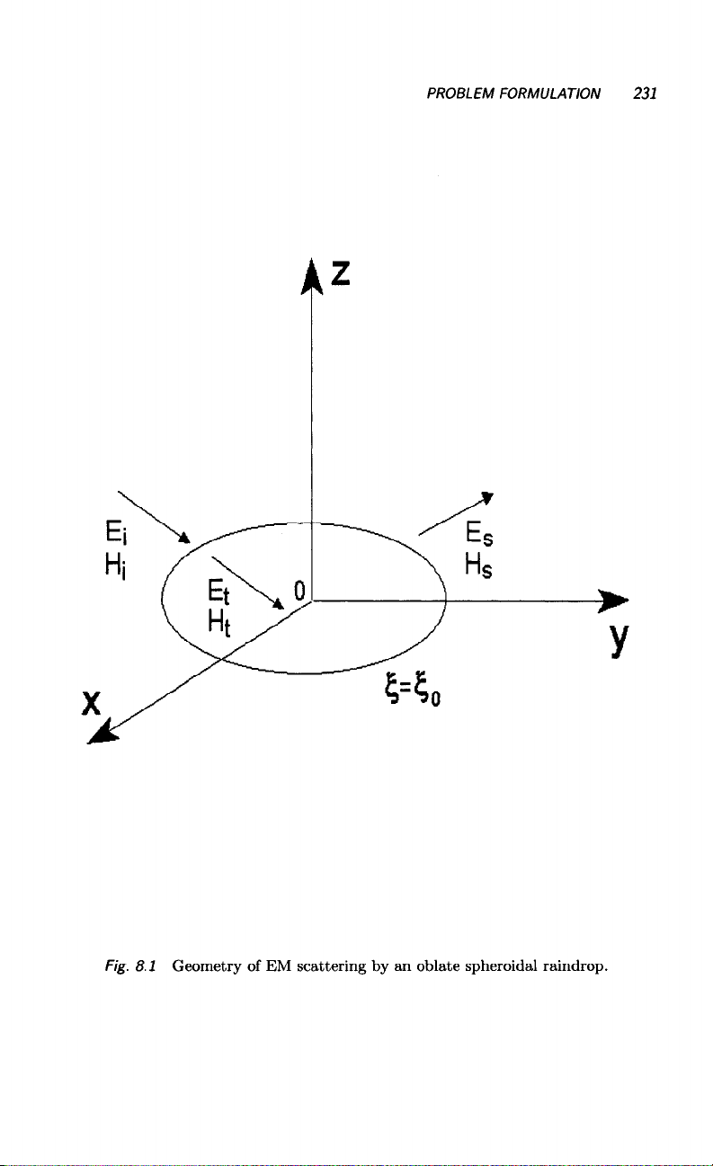
230 ANALYSIS OF RAINFALL ATTENUATION USlNG OBLATE RAlNDROPS been done in this area, with many different configurations explored. The for- mulations presented in this chapter closely follow the work presented in [24], implying our simplification to that of scattering by a single oblate raindrop. 8.2 PROBLEM FORMULATION 8.2.1 Geometry of the Problem Consider the geometry where an incident plane EM wave is scattered by an oblate spheroidal raindrop in a homogeneous, isotropic medium, as shown in Fig. 8.1. The E field is in the plane of incidence in the case of vertical polarization (TM) mode. The Ii field is in the plane of incidence in the case of horizontal polarization (TE mode). It is no doubt that both E and H fields inside and outside the raindrop satisfy Maxwell’s equations. 8.2.2 Definition of the EM Field It is obvious that the EM fields here can be expressed in the same way - as the spheroidal wave function expansions - as in previous chapters. In this chapter we expand the incident, scattered, and transmitted EM fields in terms of another type of oblate spheroidal wave vector, M(r) and N(r). Their complete definitions in terms of spheroidal coordinates T are given in Appendix A. Two casesof polarizations are considered, the TE mode and the TM mode. 8.2.2.1 Case 1: TE Mode Incident field Ei = 2 2 in [9,,(-ic,O)M~~~n(-ic,iF) n=m m=O (&la) (&lb) where M$zn ( -ic, is) and N$&( -ic, it) are presented in Appendix A (in which the barameters c and c are replaced by -ic and it, respectively, for the
PROBLEM FORMULATlON 231 Fig. 8.1 Geometry of EM scattering by an oblate spheroidal raindrop.
232 ANALYSIS OF RAINFALL ATTENUAT/ON WNG OBtATE RAINDROPS oblate case), and 49-n =)I dy-y-ic) p,“+r @OS0) fmn(-ic,q = - c (8.2a) A mn r=O,l (T + m)(r + m + 1) sin8 ’ l with Pr (cost9) denoting the associated Legendre functions and m+r 00 A mn = rx o : (2r + 2m + l)r! 2(r + 2m)! pmn(-~c)j2e ’ (8.3) = 7 When 0 = 0, only the terms with m = 1 remain, and hence fin(O) = gin(O) = $ gfd:n(-iC) mn r=O,l Scattered field E, = 2 5 in [&,mn(-ic,e)M:~~n(-~c,i~) n=m m=O + ial,mn(-iC,8)N$zn(- 9 w l ) 41 l ) (8.4a) H, = & 2 2 in [OLl,mn(-iC,B)M~~~n(-ic,iE) n=m m=O - @l ,mn(-ic7e)N~‘$-jn(-’ 7 ix 9 a] l 7 (8.4b) where al,mn and Pl,mn are unknown coefficients to be determined from the boundary conditions. Transmitted field Et = 5 2 in [61,mn(-i~,0)M~~~n(-i~,i~) n=m m=O + iyl,mn(-ic, e)NTg(zn(- 7 zc ) 4] ’ ’ ) (8.5a) Ht = JG 5 2 in [n,,,(-ic,t?)M$&(-ic,iJ) n=m m=O - iSl,mn(-iC, e)NL(zn(- 7 2c 9 zs,] ’ ’ 7 (8.5b) where Yl,mn and Sl,mn are unknown coefficients to be determined from the boundary conditions.
PROBLEM FORMULATION 233 8.2.2.2 Case 2: TM Mode Incident field (8.6a) H i= - fi 5 2 in [gmn(-ic,B)M~~~n(-ic,i~) n=m m=O + ifmn(-iC,tY)N~‘~,(-’ 7 2c, 2F)] ,l (8.6b) where fmn and gmn are expressed in Eqs. (8.2a) and (8.2b), respectively. Scattered field n=m m=O (8.7a) H s= - & 2 2 in [Rz,,, (-ic, e)M$Z$( 1 -ic, i
234 ANALYSIS OF RAlNFALl. ATTENUATION USING OBLATE RAlNDROPS 8.2.3 Boundary Conditions and Solution of Unknowns At the surface of a spheroidal raindrop (i.e., < =
PROBLEM FORMULATION 235 + fmnx:;t (-ice) + gmn Y(1)9t (-ic()) mn 1 =e in[&~l,mnX~~t(-iC1) n=m +&6l,mnY~~‘“(-icl,] ; (8.10d) TM mode 00 2l n 12Z,mnU,,it(-iC~) + &,mnVi$9t(-iC()) x [ n=m + 00 fmnUzkt (-ice) + g 77-m Wq-ic()) mn 1 - >:in [yz,mnUIit (-iCl) + 6Z,mnVn)lt (-iCl) 19 (8.11a) n=m + fmnXzkt (-ic()) + g mn Y(Qt (-ic()) mn 00 - c in[yz,mnXzkt(-iCl) J +6~,mnY~Jyt(-icl) 17 (8.11b) n=m 00 x a [*~,mnV~~‘t n=m n l (-iC()) + pz,mnUI.t (-iC()) + fmnV$$‘t (-ice) + g mn wq-ic()) mn 1 = 2 in [ &~~,mnVY$!iyt(-iCl) + J;;a,,mnU~~t(-icl,] 3 n=m (8.11~) n=m n=m (8.11d)
236 ANALYSIS OF RAINFALL ATTENUATION USING OBLATE RAINDROPS In Eqs. (8.lOa) to (8.lld), Ugkt, Viit, X$& and Yii” are defined as: for m > 1, - ug;t (-ic) = m&)R$Q-ic,&) l [(g + 1)21$yic) - 2( - x [-2I3-ic) + ($f + l)Iygy-ic) - I$yic)] + R&(‘ic,i
PROBLEM FORMULATION 237 (813c) . ot Y0;’ = 0 9 (8.13d) where Itmtn is defined in Appendix B, where parameter c for a prolate spheroid should be replaced by -ic for an oblate spheroid. 8.2.4 Total Cross Section The extinction total cross section (TCS) is defined as the ratio of the sum of absorbed and scattered energy flow of the incident waves, or alternatively, as the sum of absorption and scattering cross sections. For spherical (or small) raindrops, calculation of the TCS is straightforward and is given by Q= -- 27r ~(2772 + 1) Re[S& + Sh], O” (8.14) k2 m=l 0 where a- Sme- &&P) [~j&)l - j&d Kh-dCdl (8.15a) Sb jn(p> (Cdl - C2jn [Pjn KPjn (Cd WI (8.15b) rn=- while 5 is the complex refractive index of the raindrop that is calculated from Etay’s FORTRAN program [4]; p = Icea, where IQ is the complex propagation constant of the raindrop and a is its radius, jn is the Bessel function of the first kind, and hp) is the Hankel function of the second kind. For an oblate-shaped raindrop, the TCS is defined as follows: TE mode C1,ext = -TRe g 2 [al,mn l arnn + Pl,mn l Xmn] y (8.16) n=m m=O TM mode c2,ext = 2 2 [QIZ,mn ’ ornn + P2,mn ’ xmn] 7 (8.17) n=m m=O
238 ANALYSIS OF RAINFALL ATTENUATION USING OBLATE RAINDROPS = msmn(c’ cos0) ornn sin8 ’ dSmn(CT 0) cos Xmn = . de For parallel incidence (i.e., 8 = 0), the TCS values for the TE and TM modes reduce to c ext = -TFte 2 2 [Q12,mn l amn(O) + P2,mn ’ Xmn(O>] 3 @*W { n=m m=O 1 0 mZ1, ~mn(0) = xmn(0) = i fJr+l)(r+2)d:n, m=l. 7‘=0,1 After completing calculation of the TCS values, the specific at tenuation can then be determined using the relat ionship A = A0 QT(D)N(D) dD dB/km, (8.19) where A0 = 4343, QT(D) is the TCS of a raindrop of diameter D, and N(D) is the raindrop size distribution. 8.3 SIZE PARAMETERS OF RAINDROPS 8.3.1 Radius-Independent Oblate Spheroid Raindrop The easiest way to describe a deformed raindrop is to consider it as an oblate spheroid with a fixed deformation factor. In this case, the ratio of minor- radius and major radius becomesindependent of raindrop size. Kharadly and Choi [173] used this kind of radius-independent deformation factor in their calculation. To take into account the situation where the raindrop deformation factor varies with different raindrop size (i.e., the deformation factor decreases as the size of raindrop increases), they used different deformation factors at the different rain rates, assuming that the heavier the rain, the larger the average size and the smaller the deformation factor. 8.3.2 Radius-Dependent Oblate Spheroid Raindrop Other raindrop shape assumptions include the deformation factor as a radius- dependent parameter. Oguchi [168,169] obtained the theoretical results of the
NUMERICAL CALCULATION AND RESULTS 239 differential attenuation between horizontally and vertically polarized waves with the raindrop in the predicted eccentricity at terminal velocity. In this assumption, the raindrop is considered as an oblate spheroid and the surface of the spheroid is given as r= (8.20) where a is the major radius of the oblate spheroid, b is the minor radius, and v is expressed as (8.21) with z being the mean radius. Using the relationship given by Morrison and Cross [58], the relationship between the major axis b, minor axis a, and mean drop radius a can also be simplified as a - =1-Z, (8.22) b where in the oblate spheroidal coordinate system d d a= -&) and b=s 2 By using the concept of an equivolumic spherical raindrop, 4 -3 - -Tab 2 . --a 4 (8.23) 3 3 Hence the parameters d and {e can be calculated. Values of the parameters used in calculation of the total cross-section of an oblate spheroidal raindrop are listed in Tables 8.1 to 8.3. 8.4 NUMERICAL CALCULATION AND RESULTS After the solution from EM boundary conditions based on the raindrop sizes selected is obtained, the TCSs for various microwave frequencies and raindrop sizes can finally be obtained. In calculation of the matrix equation system, the truncation numbers depend on the size of the oblate spheroid and its orientation. In general, a small oblate spheroid with a small value of a/b and a small fractive index requires a smaller value of truncation number, while a large spheroid with a large value of a/b and a large refraction index requires a large truncation number. The results calculated for total cross sections are shown in Figs. 8.2 to 8.4. The truncation numbers for nz and n are increased as the raindrop size
240 ANALYSIS OF RAINFALL ATTENUATION USING OBLATE RAINDROPS Table 8.1 Inside the Raindrop: Spheroid Parameter 60 and the Confocal Distance d of Various Raindrop Sizes E(cm) :=1-z CO d (4 0.025 0.975 4.38784 0.0112044 0.050 0.950 3.04243 0.0317635 0.075 0.925 2.43442 0.0584956 0.100 0.900 2.06474 0.0902941 0.125 0.875 1.80739 0.12654 0.150 0.850 1.61357 0.166832 0.175 0.825 1.45983 0.210895 0.200 0.800 1.33333 0.258532 0.225 0.775 1.22634 0.309601 0.250 0.750 1.13389 0.364003 0.275 0.725 1.05263 0.421675 0.300 0.700 0.980196 0.482581 0.325 0.675 0.91486 0.546715 Table 8.2 Outside the Raindrop: Spheroid Parameter ~0 for Various Frequencies of Incident Waves (Air Medium) E (cm) ~0 (15 GHz) a, (21 GHz) ~0 (30 GHz) 0.025 0.0175998 0.0249038 0.0351996 0.050 0.0498938 0.0705999 0.0997879 0.075 0.0918847 0.130017 0.183771 0.100 0.141834 0.299695 0.283667 0.125 0.198768 0.281257 0.397536 0.150 0.262059 0.370814 0.524119 0.175 0.331274 0.468752 0.662548 0.200 0.406101 0.574633 0.812203 0.225 0.48632 0.688143 0.972635 0.250 0.571775 0.809062 1.14355 0.275 0.662365 0.937247 1.32473 0.300 0.758037 1.07262 1.51607 0.325 0.858778 1.21517 1.71756
NUMERICAL CALCULATION AND RESULTS 241 Table 8.3 Inside the Raindrop: Spheroid Parameter CO for Various Frequencies of Incident Waves ii (cm) ~0 (15 GHz) ~0 (21 GHz) ~0 (30 GHz) 0.025 0.1283-iO.04491 0.1610-iO.06998 0.1761 -iO.O9699 0.050 0.3637-i0.1273 0.4563-i0.1984 0.4993-iO.2750 0.075 0.6698-i0.2345 0.8403-i0.3654 0.9194-iO.5064 0.100 1.0339-i0.3619 1.2971 -iO.5640 1.4192-iO.78162 0.125 1.4489-iO.5072 1.8178-iO.7904 1.9890-il.0954 0.150 1.9102-i0.6687 2.3966-il.0420 2.6223-il.4442 0.175 2.4147-i0.8453 3.0296-il.0420 3.3149-il.8256 0.200 2.9602-il.0362 3.7140-il.6148 4.0636-i2.2379 0.225 3.5449-1.2409 4.448-il.9338 4.8663-i2.6800 0.250 4.1678-il.4589 5.2291 -i2.2736 5.7214-i3.1509 0.275 4.8281 -il.6901 6.0576-i2.6338 6.6279-i3.6502 0.300 5.5255-1.9342 6.9326-i3.0142 7.5852-i4.1774 0.325 6.2598-i2.1913 7.8539-i3.4148 8.5933-i4.7326 increases in order to achieve convergence in the final results. In Figs. 8.2 and 8.3, the TCS values of a raindrop from Mie scattering is also plotted for comparison. As expected, deviation of the oblate spheroidal raindrop TCS from that of an equivolumic Mie spherical raindrop increases as the raindrop size increases. This is due to the fact that raindrops are spheres at small sizes but are better described by distorted spheroids at large sizes. Calculations reveal that the TCS values at large sizes are larger than that of a Mie sphere for the TE mode but smaller for the TM mode. Figure 8.4 shows a comparison of the TCS results calculated with those obtained by Morrison and Cross [58]. It can be seenthat for both the TE and TM modes, the TCS values obtained here are larger than those computed by Morrison and Cross. It is found that the contribution to the TCS due to the raindrop distor- tions is no longer small enough to be neglected, because when the raindrop becomes bigger, distortion of the large-dimension raindrops affects the TCS significantly.
242 AA/ALYSlS OF RAlNFALL ATTEWATION USING OBLATE RAlNUROPS 0.8 -- I 1.0 2.0 5 (cm) (a) TE mode - Spheroid w-m- Mie 0.8 -- -.--. . ------ - _-_.- i 0.6 ---I -_ 1.0 2.0 Z (cm) (b) TM mode Fig. 8.2 TCS of an oblate spheroidal raindrop at 15 GHz.
NUMERICAL CALCULATION AND RESULTS 243 1.6 l 0.8 --. 0.0 1 .o 2.0 Z (cm) (a) TE mode 0.8 1 --_ ^- _-- __ ..-. .-. -_- -. ._ - .-. - Spheroid i -mm- Mie 0.6 .-- 0.0 1 .o 2.0 a (cm) (b) TM mode Fig. 8.3 TCS of an oblate spheroidal raindrop at 21 GHz.
244 ANALYSIS OF RAINFALL ATTENUATION USING OBLATE RAINDROPS 0.8 -- i 1.0 2.0 3.0 Z (cm) (a) TE mode 1.6 .- -..- -.- -.-.- _ -_- .- -- _-_-. - - Spheroid ---- Morrison 1.2 ~ --- I 0.8 -~- 0.4 ---. 0.0 --t--- - 1 .o 2.0 Z (cm) (b) TM mode Fig. 8.4 TCS of an oblate spheroidal raindrop at 30 GHz.