
CÔNG NGHỆ https://jst-haui.vn
Tạp chí Khoa học và Công nghệ Trường Đại học Công nghiệp Hà Nội Tập 60 - Số 11 (11/2024)
48
KHOA H
ỌC
P
-
ISSN 1859
-
3585
E
-
ISSN 2615
-
961
9
ISDNN: A DEEP NEURAL NETWORK FOR CHANNEL ESTIMATION
IN MASSIVE MIMO SYSTEMS
ISDNN: MẠNG NƠ-RON SÂU CHO ƯỚC LƯỢNG KÊNH HỆ THỐNG MASSIVE MIMO
Do Hai Son1, Vu Tung Lam2,
Tran Thi Thuy Quynh2,*
DOI: http://doi.org/10.57001/huih5804.2024.366
1. INTRODUCTION
Massive MIMO is an
essential technology in 5G
and beyonds. This
technology offers
significant improvements
in spectral efficiency and
capacity by exploiting a
large number of antennas
to serve multiple users
simultaneously. Moreover,
with the base station (BS)
employing thousands of
antennas, the wireless
channel experiences
channel hardening
characterized by
predominant large-scale
fading effects and
extended coherence time
[1]. However, the
proliferation of antennas
also leads to more
complexity during the CE
phase due to the intricate
structure of the channel
matrix, which may not
always exhibit full rank.
Thus, low-complexity CE
algorithms have attracted a
lot of studies.
In this paper, we focus
on applying deep learning
(DL), a trending approach,
ABSTRACT
Massive Multiple-Input Multiple-
Output (massive MIMO) technology stands as a cornerstone in 5G and beyonds.
Despite the remarkable advancements offered by massive MIMO technology, the extreme number of antennas introduces
challenges during the channel estimation (CE) phase. In this paper, we propose a single-
step Deep Neural Network (DNN)
for CE, termed Iterative Sequential DNN (ISDNN), inspired by recent developments in data detection algorithms. ISDNN is a
DNN based on the projected gradient descent algor
ithm for CE problems, with the iterative iterations transforming into a
DNN using the deep unfolding method. Furthermore, we introduce the structured channel ISDNN (S-
ISDNN), extending
ISDNN to incorporate side information such as directions of signals and
antenna array configurations for enhanced CE.
Simulation results highlight that ISDNN significantly outperforms another DNN-
based CE (DetNet), in terms of training time
(13%), running time (4.6%), and accuracy (0.43 dB). Furthermore, the S-ISDNN demonstrates
even faster than ISDNN in
terms of training time, though its overall performance still requires further improvement.
Keywords: Massive MIMO, channel estimation, single-
step Deep Neural Network, unstructured/structured channel
model.
TÓM TẮT
Massive MIMO là một công nghệ nền tảng được sử dụng trong các hệ thống truyền thông 5G trở lên. Mặc d
ù
mang lại nhiều lợi thế nhưng công nghệ này cũng gặp thách thức lớn về độ phức tạp tính toán trong pha ước lư
ợng
kênh do số lượng rất lớn các phần tử anten trong mảng. Bài báo này đề xuất một mạng nơ-ron sâu đơn bước mở, đư
ợc
đặt tên là ISDNN (Iterative Sequential Deep Neural Network) nhằm cải thiện độ phức tạp tính toán trong ước lư
ợng
kênh massive MIMO. Ý tưởng xây dựng ISDNN là áp dụng kỹ thuật trải sâu cho một giải thuật lặp để ước lượng k
ênh,
mỗi lớp trong mạng thực thi một lần lặp, các thông số vào ban đầu được tính dựa trên thuật toán ước lư
ợng phổ biến
LS (Least Square). Hơn nữa, bài báo cũng thực hiện việc mở rộng ISDNN thành S-ISDNN (structured cha
nnel ISDNN)
để áp dụng cho trường hợp kênh có cấu trúc. Kết quả nghiên cứu chỉ ra rằng, việc sử dụng ISDNN vư
ợt trội khi so sánh
với một mô hình mạng đã được đề xuất trước đây là DetNet, về thời gian đào tạo (13%), thời gian chạy (4,6%), và độ
chính xác (tốt hơn 0,43dB). Hơn nữa, S-ISDNN còn có thời gian đào tạo nhanh hơn so với ISDNN, mặc dù hiệ
u năng
tổng thể của nó vẫn cần được cải thiện thêm.
Từ khóa: MIMO siêu lớn, ước lượng kênh, mạng nơ-ron sâu một bước, mô hình kênh không sử dụng cấu trúc/có cấu trúc.
1Information Technology Institute, Vietnam National University, Hanoi, Vietnam
2University of Engineering and Technology, Vietnam National University, Hanoi, Vietnam
*Email: quynhttt@vnu.edu.vn
Received: 03/7/2024
Revised: 25/9/2024
Accepted: 28/11/2024

P-ISSN 1859-3585 E-ISSN 2615-9619 https://jst-haui.vn SCIENCE - TECHNOLOGY
Vol. 60 - No. 11 (Nov 2024) HaUI Journal of Science and Technology 49
in CE for massive MIMO systems [2]. In one of the first
studies [3], the authors employed a convolutional neural
network (CNN) to estimate the channel in millimeter
wave (mmWave) massive MIMO systems. This work used
combining matrix, beamforming matrix, and assuming
pilot sequences are all a constant value to pre-estimate a
“tentatively estimated channel”. The CNN network
corresponds to denoising a quasi-accurate channel. In [4],
the authors proposed to use an Auto-Encoder network
for CE. In this study, pilot sequences are randomly
generated. Therefore, at the first step of CE, [4] remove
known pilots from received signals using an inverse
transformation (Least-square method). Likewise, [5] used
a deep neural network (DNN) to first denoise the received
signal, followed by a conventional least-squares (LS)
estimation. In these studies, a common aspect is the
requirement for two steps for CE, such as (i) removing the
known pilot signal from the received signal and (ii) the
precise estimation of the channel.
Inspired by data detection algorithms in [6, 7], we
propose a single-step DNN for CE, namely ISDNN
(Iterative Sequential Deep Neural Network). We convert
the iterative sequential algorithm in [7] to a DNN by the
deep unfolding method [8] and modify the structure of
DNN to achieve better accuracy. In addition, the
complexity of ISDNN is reduced since it does not require
the inversion/pseudo-inversion operation as an LS
estimator. Instead, ISDNN approximates this operation
through the learning process. This paper also extends
ISDNN to S-ISDNN (structured channel ISDNN) for
estimating mm-wave channels with known directions of
arrival and array geometry (side information). The mm-
wave channel is usually applied for next-generation
wireless communications and named as “structured
channel” with few dominant rays, also used in our
previous research [9]. According to simulation results, the
proposed ISDNN structure outperforms DetNet-based CE
[6] in terms of training time, running time, and accuracy.
Moreover, the S-ISDNN demonstrates even faster than
ISDNN regarding training time, but its performance
requires further improvement.
The main contribution of this paper is to propose
ISDNN and S-ISDNN estimators for CE and side
information-aided CE, respectively. The massive MIMO
system model is presented in section 2. The proposed
ISDNN and S-ISDNN are shown in section 3. Finally, we
conduct simulations to compare the performance of
ISDNN with that of another DNN-based estimator. The
source code is available at
https://github.com/DoHaiSon/ISDNN.
2. SYSTEM MODEL
In this work, we consider a massive MIMO system,
which consists of N transmit antennas and N receive
antennas (N≪N). In the up-link channel, at time n, the
Eq. (1) expresses the system model.
(
n
)
=
(
n
)
(
n
)
+
(
n
)
,
(1)
where ∈ℂ×,∈ℂ×, and ∈ℂ× are
vectors of transmit signal, receive signal, and additive
noise, respectively. We assume that the elements of (n)
are independent and identically distributed (i.i.d) random
variables following a complex normal distribution
(0,σI). The effects of wireless propagation are
represented by ∈ℂ×, a.k.a channel matrix.
Hereafter, for brevity, we omit the timestamp n. Note that
the condition N≪N is crucial. In the contrary scenario,
the CE problem, given and , becomes
underdetermined. The elements in are represented as
complex numbers, capturing both the amplitude and
phase effects induced by the channel. Without loss of
generality, complex values are often decomposed into
real (ℜ) and imaginary () parts, as follows:
=
[
ℜ
(
)
ℑ
(
)
]
;
=
[
ℜ
(
)
ℑ
(
)
]
;
=
[
ℜ
(
)
ℑ
(
)
]
;
=
ℜ
(
)
−
ℑ
(
)
ℑ
(
)
ℜ
(
)
,
(2)
with ∈ℝ×, ∈ℝ×, ∈ℝ×, and
∈ℝ×. The (.) is the transpose operator.
In the CE process, pilot sequences are organized into
three types: block-type, comb-type, and lattice-type [10].
This study adopts the block-type arrangement, where all
channels transmit pilot signals at specific time slots. This
implies a prior knowledge of and in Eq. (1) for CE.
Subsequently, the estimated channel is utilized in
multiple subsequent data time slots within a channel
coherence time [11].
In the estimation process, ℒ;
(,) is the lost
function between the original and estimated
given
, . By using the Eq. (3), we can find the best channel
matrix.
min
ℒ
;
(
,
)
,
(3)
where and are the expectation value and learning
values, respectively.
3. THE PROPOSED ISDNN
3.1. The architecture of the proposed ISDNN
The optimal solution to solve Eq. (3) is the Maximum-
likelihood estimator (MLE), as follows:
CÔNG NGHỆ https://jst-haui.vn
Tạp chí Khoa học và Công nghệ Trường Đại học Công nghiệp Hà Nội Tập 60 - Số 11 (11/2024)
50
KHOA H
ỌC
P
-
ISSN 1859
-
3585
E
-
ISSN 2615
-
961
9
(
,
)
=
arg
min
|
−
|
,
∈
ℝ
×
(4)
However, the computational complexity of MLE
increases exponentially with N and N. Thus, it is
unfeasible to deploy it in the massive MIMO system of
interest. Inspired by [6], the projected gradient descent
(PGD) method and chain rule are used to solve the Eq. (4).
The solution is given by Eq. (5).
=
−
δ
∂
∥
−
∥
∂
=
−
δ
+
δ
,
(5)
where
is the estimated channel matrix at the k-th
iteration, for k = 1,…,K. is a non-linear operator and
δ is the learning rate. In [6], the authors unfolded this
iterative solution to a DNN structure, named DetNet, for
data detection problems. In this paper, we propose a new
structure of the network for channel estimation, called
ISDNN.
In [6], the authors initialized
by a zeros matrix.
However, [13] pointed out that by taking advantage of
the LS estimator, the learning process can be accelerated.
The formula of LS-based estimator is expressed by Eq. (6).
=
(
)
=
.
(6)
Note that due to the transformation in Eq. (2), the
Hermitian operator (.) is turned into transpose. We
denote = and =. The diagonal elements of
are combined into a diagonal matrix =diag(). At
the initialization step, the initial to be input to the first
layer of ISDNN is given by Eq. (7).
=
.
(7)
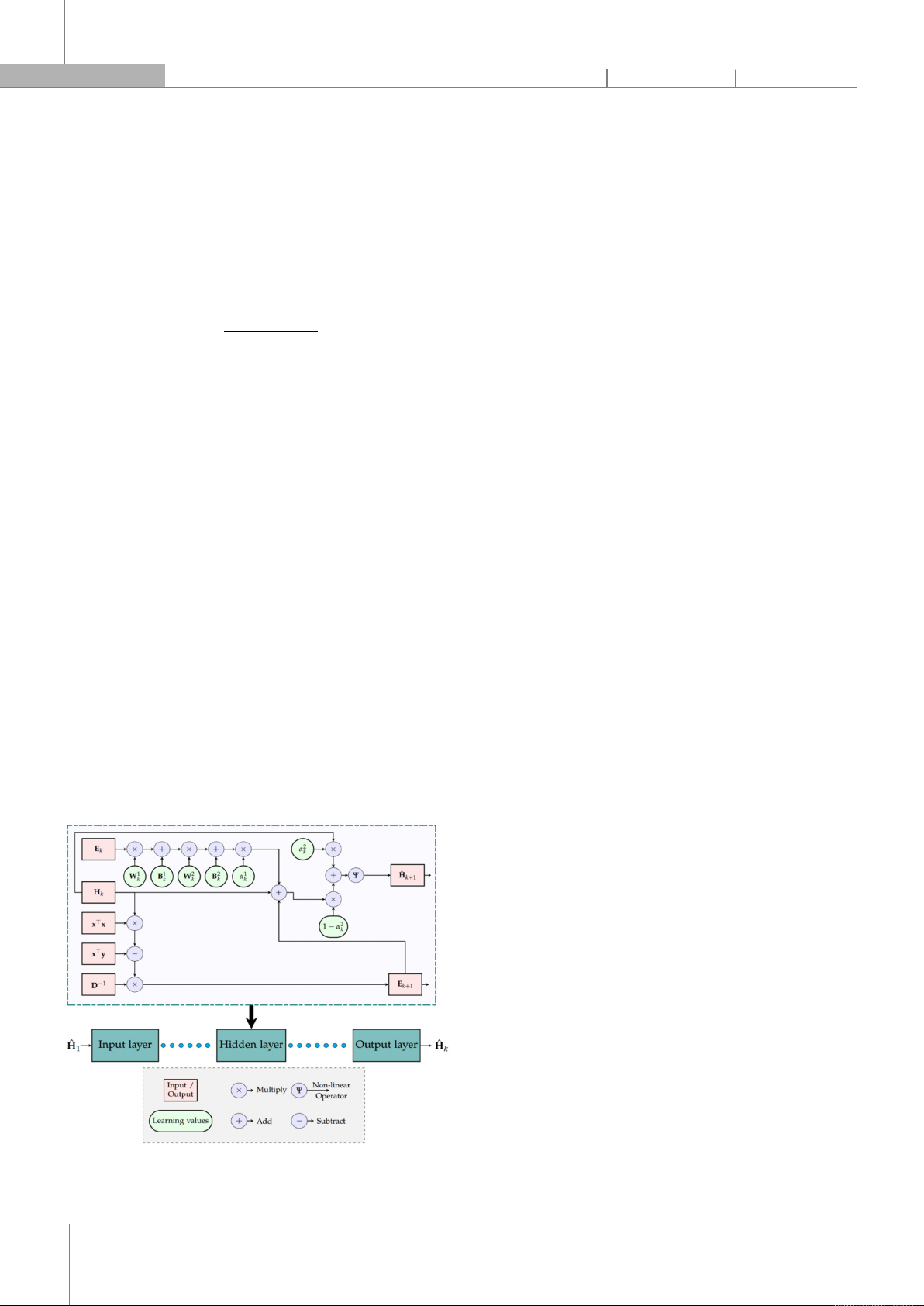
Figure 1. The architecture of a layer in the proposed ISDNN network
Figure 1 shows the architecture of a layer in our
proposed ISDNN network. From the ISDNN’s second layer
onwards,
is residual matrix at j-th iteration and k-th
layer can be computed by Eq. (8).
=
−
,
(8)
Note that, in [7], the authors proved that |
|<
|
| for the data detector problems. Hence, the distance
between and
is reduced after iterations. After any
layer, ISDNN [7] updates the estimated
by Eq. (9).
=
+
,
(9)
The in Eq. (9) can be re-write as the decomposed
approach: x=x+x, as follows:
=
−
.
(10)
However,
depends on not only as shown in
Eq. (9) but also residual matrices from previous layers, i.e.,
, ,…, . Nevertheless, due to the highest
correlation between neighboring residual matrices, the
ISDNN only considers the influence of at the k-th layer.
Thus, we add a learning value α
to each ISDNN layer to
show residual matrices’ impacts.
=
+
+
α
.
(11)
Moreover, we do not directly assign
=.
We use the convex combination [12] of and
with
learning values α
to consider the association between
them. In this way,
is contributed by both and
in α
ratio. Eq. (9) is turned into Eq. (12).
=
1
−
α
+
α
.
(12)
After that, we add two linear operators before
updating . This modification increases training time
but will also increase accuracy in the case of complex
channels.
←
+
+
.
(13)
where and are matrices of weight and bias in a
Pytorch framework linear function.
The detectors in [6, 7, 13] sequentially feed the
training data corresponding to a single sample into the
network. This significantly reduces the learning speed of
a DNN network by not leveraging the advantages of
tensor data types, which allow the manipulation of multi-
dimensional variables. Therefore, the next improvement
point of the ISDNN is to use a much larger ‘Batch size’ (bs),
where ‘bs’ represents the amount of data used in a single
iteration. The input data of the ISDNN are combined into
a 3-dimensional tensor, as follows:

P-ISSN 1859-3585 E-ISSN 2615-9619 https://jst-haui.vn SCIENCE - TECHNOLOGY
Vol. 60 - No. 11 (Nov 2024) HaUI Journal of Science and Technology 51
←
,,
,,…,
,;
←
,,
,,...,
,;
←,,,,…,,;
←,,,,…,,.
However, this is a technical programming proposal,
mathematical symbols such as matrix multiplication
notation similar to bs=1 will still be retained to avoid
confusion.
3.2. Learning process of ISDNN
The learning values of the training process are as
follows: =
,
,
,
,α
,α
|
. The
normalized mean square error (NMSE) function is utilized,
as in Eq. (14), to measure the accuracy of the ISDNN
network.
NMSE
;
(
,
)
=
∑
∑
|
h
,
−
h
,
|
∑
∑
|
h
,
|
,
(14)
where t,l are t-th transmitter and l-th receiver,
respectively. h, is the element of row t-th, column l-th in
the channel matrices and
. The four steps of an
iteration in the training phase are as follows:
1) Initialize the initial parameters and residual vectors
of the ISDNN structure: ,,α
,α
.
2) Feed the dataset through the K layers (forward
propagation), then calculate the loss through the
function built-in MSE function of Pytorch framework, as
Eq. (15).
ℒ
;
(
,
)
=
1
N
N
h
,
−
h
,
(15)
3) Back-propagate ℒ;
(,) to obtain the
gradient.
4) From the obtained gradient, ISDNN uses an
optimization algorithm, such as Adam [14], to update the
learning values .
3.3. Structured channel ISDNN
In [9, 15], the authors presented channel models, i.e.,
“unstructured” and “structured”, for massive MIMO and
mmWave systems. In the unstructured channel model,
propagation effects between transmit and receive
antenna pairs are described by complex gains, while the
structured model involves complex gains, DoA, and DoD.
The elements in are expressed as follows:
h
,
=
β
,
⋅
e
,
,
,
,
(16)
for the p-th ray, β represents complex path gain, and
“⋅” is the scalar product. Zenith and azimuth angles of
DoA are θ,ϕ, respectively. Other notations are calculated
[9] by k=2π/λ; cθ,,ϕ,=⋅;
=sinθ,cosϕ,
+sinθ,sinϕ,
+cosθ,
;
=x
+y
+z
, where λ is the wavelength; is the
unit vector in the direction of the field point; is the
position of l-th element in receiver’s antenna array
(x,y,z). In this work, we consider a simple case, which is
the line-of-sight (LoS), i.e., P=1, in terms of the
structured channel model. Hence, Eq. (1) can be given by
Eq. (17).
=
+
=
(
⋅
)
+
(17)
where , are matrices of β, and e,,,,
thanks to the property of scalar product. In 5G and
beyond wireless communication standards, DoA (, ) of
user equipments have been estimated and are available
at the BS prior to CE. Therefore, DoA together with the
configuration of the receive antenna array, is referred to
as side information in this case. The ISDNN architecture
will be modified to fit the structured channel model as
described in Eq. (16) (referred to as “structured channel
ISDNN”, S-ISDNN). That leads to instead of estimating ,
S-ISDNN will estimate . Hence, Eq. (17) can be turned
into Eq. (18).
=
+
with
β
,
=
h
,
φ
,
=
h
,
e
,
,
,
(18)
4. RESULTS AND DISCUSSION
In this section, we present the experimental analysis
of the proposed ISDNN using the simulation parameters
outlined in Table 1. Our experiments are run on a
personal computer with processor Intel Core i9-10900
@5.2 GHz, RAM of 64GB, and GPU of RTX 3090 48GB
VRAM. The ISDNN, S-ISDNN, and DetNet-based CE are
programmed in Python and the well-known PyTorch
framework. The training process is accelerated by GPU on
a computer with no other processes running. The NMSE
of trained ISDNN is the average of 100 testing times, as
shown in Eq. (19), at each SNR level. The pilot sequences
are assumed to modulate in 16-QAM type. Channel
matrices are generated as i.i.d Rayleigh channels [9]
with 0,1/√2.
NMSE
;
(
,
)
=
∑
NMSE
;
(
,
)
100
(19)
CÔNG NGHỆ https://jst-haui.vn
Tạp chí Khoa học và Công nghệ Trường Đại học Công nghiệp Hà Nội Tập 60 - Số 11 (11/2024)
52
KHOA H
ỌC
P
-
ISSN 1859
-
3585
E
-
ISSN 2615
-
961
9
Table 1. Simulation parameters of the proposed ISDNN and wireless
communications system
Parameters Specifications Parameters Specifications
Massive MIMO
system size
N
=
8
,
N
=
64
Non-linear
operator (
)
Tanh
Modulation
type
16-QAM Linear operator
(W) size
2
N
×
2
N
SNR levels of
training
dataset
[0, 5, 10, 15, 20]
dB
α
[
0
1
)
Training size 50,000 samples
α
0.5
Testing size 10,000 samples
[
0
1
)
Optimization
algorithm
Adam [14] Learning rate
δ
=
0
.
0001
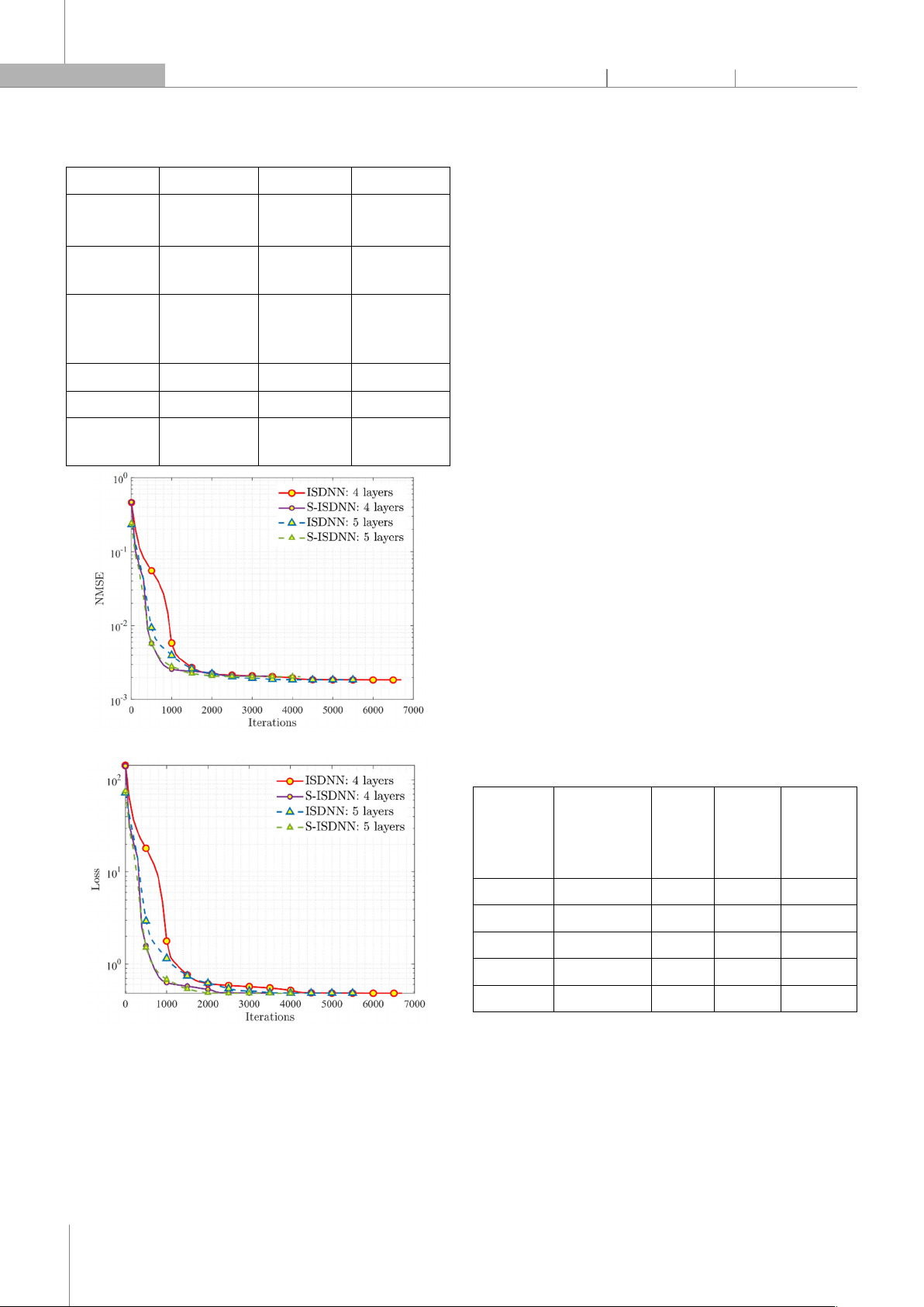
(a) NMSE
(b) Loss
Figure 2. Training process of ISDNN and S-ISDNN
Figure 2 illustrates the convergence of proposed
ISDNN and S-ISDNN with the configuration of 4 and 5
layers. We do not train ISDNN by a fixed number of
iterations but employ the “early stopping” function. As a
result, if NMSE fails to decrease for 3 consecutive
iterations, the training phase is terminated. In Figure 2a,
in terms of accuracy, ISDNN with 4 layers is the best
model with the latest NMSE 0.00184. The ISDNN with 5
layers ranks second with the latest NMSE 0.00185. In
spite of side information-aided during the CE process,
NMSEs of S-ISDNN networks are not as good as expected.
The S-ISDNN with 4 and 5 layers have the latest NMSE
values at 0.00209 and 0.00206, respectively. Regarding
iteration, ISDNN with 4 and 5 layers and S-ISDNN with 4
and 5 layers, respectively, need 6700, 5600, 3400, and
4200 iterations to converge. Nonetheless, Table 2 reveals
that fewer iterations do not necessarily equate to faster
training time. Because the time per iteration of ISDNN, S-
ISDNN with 4 layers is faster than that of ISDNN, S-ISDNN
with 5 layers. The ISDNN and S-ISDNN consist of 4 layers,
saving around 30% of training time compared to those
with 5 layers. Additionally, despite its lower accuracy, S-
ISDNN only needs half the number of iterations
compared to ISDNN with 4 layers to converge. This can
also be a trade-off during the training process. Figure 2b
describes values of ℒ;
(,) computed by the MSE
function. First, we can observe the same trend as NMSE in
Figure 2a when ℒ of ISDNN with 4 layers is the lowest. The
latest loss values of ISDNN with 4, 5 layers and S-ISDNN
with 4, 5 layers are 0.482667, 0.484506, 0.483979, and
0.481773, respectively. These values are approximately
the same since loss values directly express the coverage
of models.
Table 2. Complexity of estimators
Estimator Computational
complexity
Learning
values
Training
time
(seconds)
Running
time
(seconds /
sample)
DetNet: K = 4
(
N
N
)
263,688 46,972.63 1.34943*10-3
ISDNN: K = 4
(
N
N
)
132,104 9,416.92 6.23742*10-5
ISDNN: K = 5
(
N
N
)
165,130 11,134.20 1.33405*10-4
S-ISDNN: K = 4
(
N
N
)
132,104 6,088.08 9.53519*10-5
S-ISDNN: K = 5
(
N
N
)
165,130 8,157.22 1.40340*10-4
Table 2 shows the cost of DetNet-based CE, ISDNN, and
S-ISDNN, in terms of computational complexity, number of
learning values, training time, and running time. All
considered estimators share the same computational
complexity measured by Big-O notation at (NN
). The
computational complexities of traditional estimators, i.e.,
LS and MMSE (Minimum Mean Square Estimation), are


![Bài giảng Vi điều khiển Nguyễn Huy Hoàng: Tổng hợp kiến thức [Chuẩn nhất]](https://cdn.tailieu.vn/images/document/thumbnail/2026/20260316/hoatrami2026/135x160/72211773806757.jpg)


![Bài giảng Tự động hoá thiết bị điện [chuẩn nhất]](https://cdn.tailieu.vn/images/document/thumbnail/2026/20260312/hoabattu2026/135x160/61691773631881.jpg)
