4 IEEE TRANSACTIONS ON EVOLUTIONARY COMPUTATION, VOL. 15, NO. 1, FEBRUARY 2011
Differential Evolution: A Survey of the
State-of-the-Art
Swagatam Das, Member, IEEE, and Ponnuthurai Nagaratnam Suganthan, Senior Member, IEEE
Abstract—Differential evolution (DE) is arguably one of the
most powerful stochastic real-parameter optimization algorithms
in current use. DE operates through similar computational steps
as employed by a standard evolutionary algorithm (EA). How-
ever, unlike traditional EAs, the DE-variants perturb the current-
generation population members with the scaled differences of
randomly selected and distinct population members. Therefore,
no separate probability distribution has to be used for generating
the offspring. Since its inception in 1995, DE has drawn the at-
tention of many researchers all over the world resulting in a lot of
variants of the basic algorithm with improved performance. This
paper presents a detailed review of the basic concepts of DE and
a survey of its major variants, its application to multiobjective,
constrained, large scale, and uncertain optimization problems,
and the theoretical studies conducted on DE so far. Also, it
provides an overview of the significant engineering applications
that have benefited from the powerful nature of DE.
Index Terms—Derivative-free optimization, differential evolu-
tion (DE), direct search, evolutionary algorithms (EAs), genetic
algorithms (GAs), metaheuristics, particle swarm optimization
(PSO). I. Introduction
TO TACKLE complex computational problems, re-
searchers have been looking into nature for years—both
as model and as metaphor—for inspiration. Optimization is at
the heart of many natural processes like Darwinian evolution
itself. Through millions of years, every species had to adapt
their physical structures to fit to the environments they were
in. A keen observation of the underlying relation between
optimization and biological evolution led to the development
of an important paradigm of computational intelligence—the
evolutionary computing techniques [S1]–[S4] for performing
very complex search and optimization.
Evolutionary computation uses iterative progress, such as
growth or development in a population. This population is then
selected in a guided random search using parallel processing
to achieve the desired end. The paradigm of evolutionary
computing techniques dates back to early 1950s, when the idea
Manuscript received September 17, 2009; revised March 9, 2010 and June
10, 2010; accepted June 12, 2010. Date of publication October 14, 2010;
date of current version February 25, 2011. This work was supported by the
Agency for Science, Technology, and Research, Singapore (A∗Star), under
Grant #052 101 0020.
S. Das is with the Department of Electronics and Telecommunication
Engineering, Jadavpur University, Kolkata 700 032, India (e-mail: swagatam-
das19@yahoo.co.in).
P. N. Suganthan is with the School of Electrical and Electronic En-
gineering, Nanyang Technological University, 639798, Singapore (e-mail:
epnsugan@ntu.edu.sg).
Color versions of one or more of the figures in this paper are available
online at http://ieeexplore.ieee.org.
Digital Object Identifier 10.1109/TEVC.2010.2059031
to use Darwinian principles for automated problem solving
originated. It was not until the sixties that three distinct
interpretations of this idea started to be developed in three
different places. Evolutionary programming (EP) was intro-
duced by Lawrence J. Fogel in the USA [S5],1while almost
simultaneously. I. Rechenberg and H.-P. Schwefel introduced
evolution strategies (ESs) [S6], [S7] in Germany. Almost a
decade later, John Henry Holland from University of Michigan
at Ann Arbor, devised an independent method of simulating
the Darwinian evolution to solve practical optimization prob-
lems and called it the genetic algorithm (GA) [S8]. These areas
developed separately for about 15 years. From the early 1990s
on they are unified as different representatives (“dialects”) of
one technology, called evolutionary computing. Also since the
early nineties, a fourth stream following the same general ideas
started to emerge—genetic programming (GP) [S9].
Nowadays, the field of nature-inspired metaheuristics is
mostly constituted by the evolutionary algorithms [compris-
ing of GAs, EP, ESs, GP, differential evolution (DE), and
so on] as well as the swarm intelligence algorithms [e.g.,
ant colony optimization (ACO), particle swarm optimization
(PSO), Bees algorithm, bacterial foraging optimization (BFO),
and so on [S10]–[S12]]. Also the field extends in a broader
sense to include self-organizing systems [S13], artificial life
(digital organism) [S14], memetic and cultural algorithms
[S15], harmony search [S16], artificial immune systems [S17],
and learnable evolution model [S18].
The DE [72], [73], [88]–[90] algorithm emerged as a very
competitive form of evolutionary computing more than a
decade ago. The first written article on DE appeared as a
technical report by R. Storn and K. V. Price in 1995 [88].
One year later, the success of DE was demonstrated at the
First International Contest on Evolutionary Optimization in
May 1996, which was held in conjunction with the 1996 IEEE
International Conference on Evolutionary Computation (CEC)
[89]. DE finished third at the First International Contest on
Evolutionary Optimization (1st ICEO), which was held in
Nagoya, Japan. DE turned out to be the best evolutionary
algorithm for solving the real-valued test function suite of the
1st ICEO (the first two places were given to non-evolutionary
algorithms, which are not universally applicable but solved
the test-problems faster than DE). Price presented DE at the
Second International Contest on Evolutionary Optimization in
1Due to space limitation the supplementary reference list cited as [Sxxx]
will not be published in print, but as an on-line document only.
1089-778X/$26.00 c
2010 IEEE

DAS AND SUGANTHAN: DIFFERENTIAL EVOLUTION: A SURVEY OF THE STATE-OF-THE-ART 5
1997 [72] and it turned out as one of the best among the
competing algorithms. Two journal articles [73], [92] describ-
ing the algorithm in sufficient details followed immediately in
quick succession. In 2005 CEC competition on real parameter
optimization, on 10-D problems classical DE secured 2nd
rank and a self-adaptive DE variant called SaDE [S201]
secured third rank although they performed poorly over 30-D
problems. Although a powerful variant of ES, known as restart
covariance matrix adaptation ES (CMA-ES) [S232, S233],
yielded better results than classical and self-adaptive DE, later
on many improved DE variants [like improved SaDE [76],
jDE [10], opposition-based DE (ODE) [82], DE with global
and local neighborhoods (DEGL) [21], JADE [118], and so on
that will be discussed in subsequent sections] were proposed in
the period 2006–2009. Hence, another rigorous comparison is
needed to determine how well these variants might compete
against the restart CMA-ES and many other real parameter
optimizers over the standard numerical benchmarks. It is also
interesting to note that the variants of DE continued to secure
front ranks in the subsequent CEC competitions [S202] like
CEC 2006 competition on constrained real parameter opti-
mization (first rank), CEC 2007 competition on multiobjective
optimization (second rank), CEC 2008 competition on large
scale global optimization (third rank), CEC 2009 competition
on multiobjective optimization (first rank was taken by a
DE-based algorithm MOEA/D for unconstrained problems),
and CEC 2009 competition on evolutionary computation in
dynamic and uncertain environments (first rank). We can also
observe that no other single search paradigm such as PSO was
able to secure competitive rankings in all CEC competitions.
A detailed discussion on these DE-variants for optimization in
complex environments will be provided in Section V.
In DE community, the individual trial solutions (which con-
stitute a population) are called parameter vectors or genomes.
DE operates through the same computational steps as em-
ployed by a standard EA. However, unlike traditional EAs,
DE employs difference of the parameter vectors to explore the
objective function landscape. In this respect, it owes a lot to its
two ancestors namely—the Nelder-Mead algorithm [S19], and
the controlled random search (CRS) algorithm [S20], which
also relied heavily on the difference vectors to perturb the
current trial solutions. Since late 1990s, DE started to find
several significant applications to the optimization problems
arising from diverse domains of science and engineering.
Below, we point out some of the reasons why the researchers
have been looking at DE as an attractive optimization tool
and as we shall proceed through this survey, these reasons
will become more obvious.
1) Compared to most other EAs, DE is much more sim-
ple and straightforward to implement. Main body of
the algorithm takes four to five lines to code in any
programming language. Simplicity to code is important
for practitioners from other fields, since they may not be
experts in programming and are looking for an algorithm
that can be simply implemented and tuned to solve their
domain-specific problems. Note that although PSO is
also very easy to code, the performance of DE and its
variants is largely better than the PSO variants over
a wide variety of problems as has been indicated by
studies like [21], [82], [104] and the CEC competition
series [S202].
2) As indicated by the recent studies on DE [21], [82],
[118] despite its simplicity, DE exhibits much better
performance in comparison with several others like G3
with PCX, MA-S2, ALEP, CPSO-H, and so on of current
interest on a wide variety of problems including uni-
modal, multimodal, separable, non-separable and so on.
Although some very strong EAs like the restart CMA-
ES was able to beat DE at CEC 2005 competition, on
non-separable objective functions, the gross performance
of DE in terms of accuracy, convergence speed, and
robustness still makes it attractive for applications to
various real-world optimization problems, where find-
ing an approximate solution in reasonable amount of
computational time is much weighted.
3) The number of control parameters in DE is very few
(Cr,F, and NP in classical DE). The effects of these
parameters on the performance of the algorithm are well-
studied. As will be discussed in the next section, simple
adaptation rules for Fand Cr have been devised to
improve the performance of the algorithm to a large ex-
tent without imposing any serious computational burden
[10], [76], [118].
4) The space complexity of DE is low as compared to
some of the most competitive real parameter optimizers
like CMA-ES [S232]. This feature helps in extending
DE for handling large scale and expensive optimization
problems. Although CMA-ES remains very competitive
over problems up to 100 variables, it is difficult to extend
it to higher dimensional problems due to its storage,
update, and inversion operations over square matrices
with size the same as the number of variables.
Perhaps these issues triggered the popularity of DE
among researchers all around the globe within a short span
of time as is evident from the bibliography of DE [37]
from 1997 to 2002. Consequently, over the past decade
research on and with DE has become huge and multifaceted.
Although there exists a few significant survey papers on
EAs and swarm intelligence algorithms (e.g., [S21]–[S25]),
to the best of our knowledge no extensive review article
capturing the entire horizon of the current DE-research
has so far been published. In a recently published article
[60], Neri and Tirronen reviewed a number of DE-variants
for single-objective optimization problems and also made
an experimental comparison of these variants on a set of
numerical benchmarks. However, the article did not address
issues like adapting DE to complex optimization environments
involving multiple and constrained objective functions, noise
and uncertainty in the fitness landscape, very large number of
search variables, and so on. Also it did not focus on the most
recent engineering applications of DE and the developments
in the theoretical analysis of DE. This paper attempts to
provide a comprehensive survey of the DE algorithm—
its basic concepts, different structures, and variants for

6 IEEE TRANSACTIONS ON EVOLUTIONARY COMPUTATION, VOL. 15, NO. 1, FEBRUARY 2011
Fig. 1. Main stages of the DE algorithm.
solving constrained, multiobjective, dynamic, and large-scale
optimization problems as well as applications of DE variants
to practical optimization problems. The rest of this paper is
arranged as follows. In Section II, the basic concepts related to
classical DE are explained along with the original formulation
of the algorithm in the real number space. Section III discusses
the parameter adaptation and control schemes for DE. Section
IV provides an overview of several prominent variants of the
DE algorithm. Section V provides an extensive survey on the
applications of DE to the discrete, constrained, multiobjective,
and dynamic optimization problems. The theoretical analysis
of DE has been reviewed in Section VI. Section VII provides
an overview of the most significant engineering applications
of DE. The drawbacks of DE are pointed out in Section VIII.
Section IX highlights a number of future research issues
related to DE. Finally, the paper is concluded in Section X.
II. Differential Evolutions: Basic Concepts and
Formulation in Continuous Real Space
Scientists and engineers from all disciplines often have to
deal with the classical problem of search and optimization.
Optimization means the action of finding the best-suited
solution of a problem within the given constraints and flex-
ibilities. While optimizing performance of a system, we aim
at finding out such a set of values of the system parameters
for which the overall performance of the system will be the
best under some given conditions. Usually, the parameters
governing the system performance are represented in a vector
like
X=[x1,x
2,x
3, ..., xD]T.For real parameter optimization,
as the name implies, each parameter xiis a real number. To
measure how far the “best” performance we have achieved,
an objective function (or fitness function) is designed for the
system. The task of optimization is basically a search for such
the parameter vector
X∗, which minimizes such an objective
function f(
X)(f:⊆
D→), i.e., f(
X∗)<f(
X) for
all
X∈, where is a non-empty large finite set serving
as the domain of the search. For unconstrained optimization
problems =D. Since max f(
X)=−min −f(
X),
the restriction to minimization is without loss of generality.
In general, the optimization task is complicated by the ex-
istence of non-linear objective functions with multiple local
minima. A local minimum f=f(
X) may be defined as
∃ε>0∀
X∈:
X−
X
<ε⇒f≤f(
X), where .
indicates any p-norm distance measure.
DE is a simple real parameter optimization algorithm. It
works through a simple cycle of stages, presented in Fig. 1.
We explain each stage separately in Sections II-A–II-D.
A. Initialization of the Parameter Vectors
DE searches for a global optimum point in a D-dimensional
real parameter space D. It begins with a randomly initiated
population of NP D dimensional real-valued parameter vec-
tors. Each vector, also known as genome/chromosome, forms
a candidate solution to the multidimensional optimization
problem. We shall denote subsequent generations in DE by
G=0,1..., Gmax. Since the parameter vectors are likely
to be changed over different generations, we may adopt
the following notation for representing the ith vector of the
population at the current generation:
Xi,G =[x1,i,G,x
2,i,G,x
3,i,G, ....., xD,i,G].(1)
For each parameter of the problem, there may be a certain
range within which the value of the parameter should be
restricted, often because parameters are related to physical
components or measures that have natural bounds (for example
if one parameter is a length or mass, it cannot be negative).
The initial population (at G= 0) should cover this range as
much as possible by uniformly randomizing individuals within
the search space constrained by the prescribed minimum
and maximum bounds:
Xmin ={x1,min,x
2,min, ..., xD,min}and
Xmax ={x1,max,x
2,max, ..., xD,max}. Hence we may initialize the
jth component of the ith vector as
xj,i,0=xj,min +randi,j [0,1] ·(xj,max −xj,min) (2)
where randi,j [0,1] is a uniformly distributed random number
lying between 0 and 1 (actually 0 ≤randi,j [0,1] ≤1) and
is instantiated independently for each component of the i-th
vector.
B. Mutation with Difference Vectors
Biologically, “mutation” means a sudden change in the
gene characteristics of a chromosome. In the context of the
evolutionary computing paradigm, however, mutation is also
seen as a change or perturbation with a random element. In
DE-literature, a parent vector from the current generation is
called target vector, a mutant vector obtained through the
differential mutation operation is known as donor vector and
finally an offspring formed by recombining the donor with
the target vector is called trial vector. In one of the simplest
forms of DE-mutation, to create the donor vector for each ith
target vector from the current population, three other distinct
parameter vectors, say
Xri
1,
Xri
2, and
Xri
3are sampled randomly
from the current population. The indices ri
1,ri
2, and ri
3are
mutually exclusive integers randomly chosen from the range
[1, NP], which are also different from the base vector index
i. These indices are randomly generated once for each mutant
vector. Now the difference of any two of these three vectors is
scaled by a scalar number F(that typically lies in the interval
[0.4, 1]) and the scaled difference is added to the third one
whence we obtain the donor vector
Vi,G . We can express the
process as
Vi,G =
Xri
1,G +F·(
Xri
2,G −
Xri
3,G).(3)
The process is illustrated on a 2-D parameter space (show-
ing constant cost contours of an arbitrary objective function)
in Fig. 2.
DAS AND SUGANTHAN: DIFFERENTIAL EVOLUTION: A SURVEY OF THE STATE-OF-THE-ART 7
Fig. 2. Illustrating a simple DE mutation scheme in 2-D parametric space.
C. Crossover
To enhance the potential diversity of the population, a
crossover operation comes into play after generating the donor
vector through mutation. The donor vector exchanges its
components with the target vector
Xi,G under this operation
to form the trial vector
Ui,G =[u1,i,G,u
2,i,G,u
3,i,G, ..., uD,i,G].
The DE family of algorithms can use two kinds of crossover
methods—exponential (or two-point modulo) and binomial (or
uniform) [74]. In exponential crossover, we first choose an
integer nrandomly among the numbers [1,D]. This integer
acts as a starting point in the target vector, from where the
crossover or exchange of components with the donor vector
starts. We also choose another integer Lfrom the interval
[1,D]. Ldenotes the number of components the donor vector
actually contributes to the target vector. After choosing nand
Lthe trial vector is obtained as
uj,i,G =vj,i,G for j=nDn+1
D, ..., n+L−1D
xj,i,G for all other j∈[1,D] (4)
where the angular brackets Ddenote a modulo function with
modulus D. The integer Lis drawn from [1,D] according to
the following pseudo-code:
L=0;DO
{
L=L+1;
}WHILE ((rand(0,1) ≤Cr) AND (L≤D)).
“Cr” is called the crossover rate and appears as a control
parameter of DE just like F. Hence in effect, probability (L=
υ)=(Cr)υ−1 for any positive integer vlying in the interval
[1, D]. For each donor vector, a new set of nand Lmust be
chosen randomly as shown above.
On the other hand, binomial crossover is performed on each
of the Dvariables whenever a randomly generated number
between 0 and 1 is less than or equal to the Cr value. In this
case, the number of parameters inherited from the donor has
a (nearly) binomial distribution. The scheme may be outlined
as
uj,i,G =vj,i,G if (randi,j [0,1] ≤Cr or j=jrand )
xj,i,G otherwise (5)
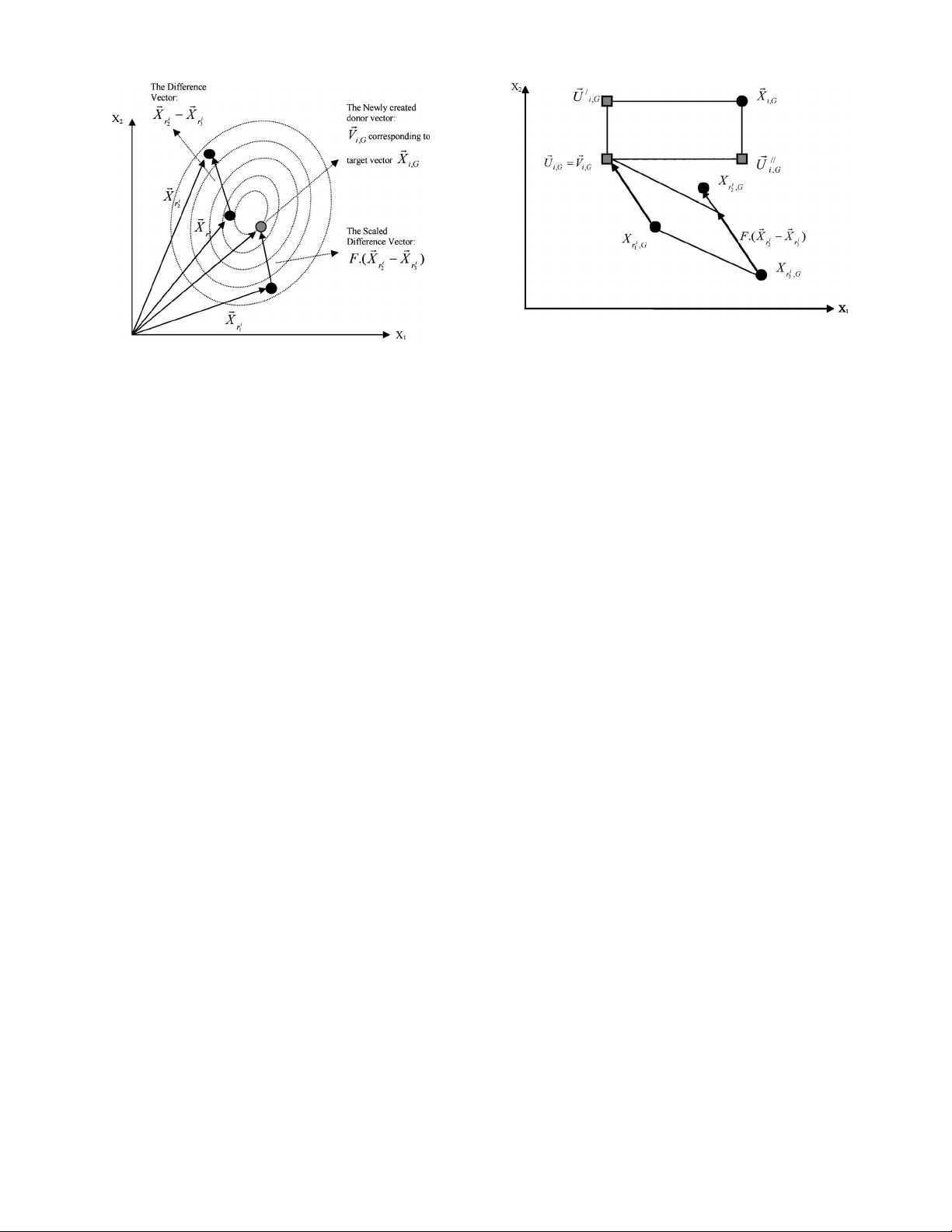
Fig. 3. Different possible trial vectors formed due to uniform/binomial
crossover between the target and the mutant vectors in 2-D search space.
where, as before, randi,j [0,1] is a uniformly distributed ran-
dom number, which is called anew for each jth component of
the ith parameter vector. jrand ∈[1,2, ...., D] is a randomly
chosen index, which ensures that
Ui,G gets at least one
component from
Vi,G . It is instantiated once for each vector
per generation. We note that for this additional demand, Cr
is only approximating the true probability pCr of the event
that a component of the trial vector will be inherited from
the donor. Also, one may observe that in a 2-D search space,
three possible trial vectors may result from uniformly crossing
a mutant/donor vector
Vi,G with the target vector
Xi,G . These
trial vectors are as follows.
1)
Ui,G =
Vi,G such that both the components of
Ui,G are
inherited from
Vi,G .
2)
U/
i,G , in which the first component (j= 1) comes from
Vi,G and the second one (j= 2) from
Xi,G .
3)
U//
i,G , in which the first component (j= 1) comes from
Xi,G and the second one (j= 2) from
Vi,G .
The possible trial vectors due to uniform crossover are
illustrated in Fig. 3.
D. Selection
To keep the population size constant over subsequent gen-
erations, the next step of the algorithm calls for selection to
determine whether the target or the trial vector survives to the
next generation, i.e., at G=G+ 1. The selection operation is
described as
Xi,G+1 =
Ui,G iff(
Ui,G )≤f(
Xi,G )
=
Xi,G iff(
Ui,G )>f(
Xi,G ) (6)
where f(
X) is the objective function to be minimized. There-
fore, if the new trial vector yields an equal or lower value
of the objective function, it replaces the corresponding target
vector in the next generation; otherwise the target is retained
in the population. Hence, the population either gets better
(with respect to the minimization of the objective function)
or remains the same in fitness status, but never deteriorates.
Note that in (6) the target vector is replaced by the trial
vector even if both yields the same value of the objective
function—a feature that enables DE-vectors to move over

8 IEEE TRANSACTIONS ON EVOLUTIONARY COMPUTATION, VOL. 15, NO. 1, FEBRUARY 2011
Algorithm 1 Pseudo-code for the DE Algorithm with Binomial
Crossover
Step 1: Read values of the control parameters of DE: scale
factor F, crossover rate Cr, and the population size NP from
user.
Step 2: Set the generation number G=0
and randomly initialize a population of NP
individuals PG={
X1,G, ......,
XNP,G}with
Xi,G =[x1,i,G,x
2,i,G,x
3,i,G, ....., xD,i,G] and each
individual uniformly distributed in the range
[
Xmin,
Xmax], where
Xmin ={x1,min,x
2,min, ..., xD,min}and
Xmax ={x1,max,x
2,max, ..., xD,max}with i=[1,2, ...., NP].
Step 3. WHILE the stopping criterion is not satisfied
DO
FOR i=1toNP //do for each individual sequen-
tially
Step 2.1 Mutation Step
Generate a donor vector
Vi,G ={v1,i,G, ......., }
{vD,i,G}corresponding to the ith target vector
Xi,G via the differential mutation scheme of DE
as:
Vi,G =
Xri
1,G +F·(
Xri
2,G −
Xri
3,G).
Step 2.2 Crossover Step
Generate a trial vector
Ui,G ={u1,i,G, ......., uD,i,G}
for the ith target vector
Xi,G through
binomial crossover in the following way:
uj,i,G =vj,i,G ,if(randi,j [0,1] ≤Cr or j=jrand )
xj,i,G , otherwise,
Step 2.3 Selection Step
Evaluate the trial vector
Ui,G
IF f(
Ui,G )≤f(
Xi,G ), THEN
Xi,G+1 =
Ui,G
ELSE
Xi,G+1 =
Xi,G .
END IF
END FOR
Step 2.4 Increase the Generation Count
G=G+1
END WHILE
flat fitness landscapes with generations. Note that throughout
this paper, we shall use the terms objective function value
and fitness interchangeably. But, always for minimization
problems, a lower objective function value will correspond
to higher fitness.
E. Summary of DE Iteration
An iteration of the classical DE algorithm consists of
the four basic steps—initialization of a population of search
variable vectors, mutation, crossover or recombination, and
finally selection. After having illustrated these stages, we now
formally present the whole of the algorithm in a pseudo-code
below.
The terminating condition can be defined in a few ways
like: 1) by a fixed number of iterations Gmax, with a suitably
large value of Gmax depending upon the complexity of the
objective function; 2) when best fitness of the population
does not change appreciably over successive iterations; and
alternatively 3) attaining a pre-specified objective function
value.
F. DE Family of Storn and Price
Actually it is the process of mutation that demarcates one
DE scheme from another. In the previous section, we have
illustrated the basic steps of a simple DE. The mutation
scheme in (3) uses a randomly selected vector
Xr1and only
one weighted difference vector F·(
Xr2−
Xr3) to perturb it.
Hence, in literature, the particular mutation scheme given by
(3) is referred to as DE/rand/1. When used in conjunction with
binomial crossover, the procedure is called DE/rand/1/bin. We
can now have an idea of how the different DE schemes are
named. The general convention used above is DE/x/y/z, where
DE stands for “differential evolution,” x represents a string
denoting the base vector to be perturbed, y is the number
of difference vectors considered for perturbation of x, and z
stands for the type of crossover being used (exp: exponential;
bin: binomial). The other four different mutation schemes,
suggested by Storn and Price [74], [75] are summarized as
“DE/best/1:
Vi,G =
Xbest,G +F·(
Xri
1,G −
Xri
2,G) (7)
“DE/target −to −best/1:
Vi,G =
Xi,G
+F·(
Xbest,G −
Xi,G )+F·(
Xri
1,G −
Xri
2,G)
(8)
“DE/best/2:
Vi,G =
Xbest,G +F·(
Xri
1,G −
Xri
2,G)
+F·(
Xri
3,G −
Xri
4,G) (9)
“DE/rand/2:
Vi,G =
Xri
1,G +F·(
Xri
2,G −
Xri
3,G)
+F·(
Xri
4,G −
Xri
5,G).(10)
The indices ri
1,ri
2,ri
3,ri
4, and ri
5are mutually exclusive
integers randomly chosen from the range [1, NP], and all are
different from the base index i. These indices are randomly
generated once for each donor vector. The scaling factor Fis
a positive control parameter for scaling the difference vectors.
Xbest,G is the best individual vector with the best fitness (i.e.,
lowest objective function value for a minimization problem) in
the population at generation G. Note that some of the strategies
for creating the donor vector may be mutated recombinants,
for example, (8) listed above basically mutates a two-vector
recombinant
Xi,G +F·(
Xbest,G −
Xi,G ).
Storn and Price [74], [92] suggested a total of ten different
working strategies for DE and some guidelines in applying
these strategies to any given problem. These strategies were
derived from the five different DE mutation schemes outlined
above. Each mutation strategy was combined with either the
“exponential” type crossover or the “binomial” type crossover.
This yielded a total of 5 ×2 = 10 DE strategies. In fact many
other linear vector combinations can be used for mutation. In
general, no single mutation method [among those described
in (3), (7)–(10)] has turned out to be best for all problems.


![Bài giảng Mạng nơ-ron nhân tạo trường Đại học Cần Thơ [PDF]](https://cdn.tailieu.vn/images/document/thumbnail/2013/20130331/o0_mrduong_0o/135x160/8661364662930.jpg)