
Engineering Applications of Artificial Intelligence 85 (2019) 845–864
Contents lists available at ScienceDirect
Engineering Applications of Artificial Intelligence
journal homepage: www.elsevier.com/locate/engappai
Heuristic design of fuzzy inference systems: A review of three decades of
research
Varun Ojha a,b,∗, Ajith Abraham c,d, Václav Snášel e
aETH Zürich, Switzerland
bUniversity of Reading, United Kingdom
cUniversity of Pretoria, South Africa
dMachine Intelligence Research Labs (MIR Labs), WA, United States
eTechnical University of Ostrava, Czech Republic
ARTICLE INFO
Keywords:
Evolutionary algorithms
Genetic fuzzy systems
Neuro-fuzzy systems
Hierarchical fuzzy systems
Evolving fuzzy systems
Multi-objective fuzzy systems
Deep fuzzy system
ABSTRACT
This paper provides an in-depth review of the optimal design of type-1 and type-2 fuzzy inference systems (FIS)
using five well known computational frameworks: genetic-fuzzy systems (GFS), neuro-fuzzy systems (NFS),
hierarchical fuzzy systems (HFS), evolving fuzzy systems (EFS), and multi-objective fuzzy systems (MFS), which
is in view that some of them are linked to each other. The heuristic design of GFS uses evolutionary algorithms
for optimizing both Mamdani-type and Takagi–Sugeno–Kang-type fuzzy systems. Whereas, the NFS combines
the FIS with neural network learning systems to improve the approximation ability. An HFS combines two
or more low-dimensional fuzzy logic units in a hierarchical design to overcome the curse of dimensionality.
An EFS solves the data streaming issues by evolving the system incrementally, and an MFS solves the multi-
objective trade-offs like the simultaneous maximization of both interpretability and accuracy. This paper ofers
a synthesis of these dimensions and explores their potentials, challenges, and opportunities in FIS research.
This review also examines the complex relations among these dimensions and the possibilities of combining
one or more computational frameworks adding another dimension: deep fuzzy systems.
1. Introduction
Research in fuzzy inference systems (FIS) initiated by Zadeh (1988)
has drawn the attention of many disciplines over the past three decades.
The success of FIS is evident from its applicability and relevance in
numerous research areas: control systems (Lee,1990;Wang and Griffin,
1996), engineering (Precup and Hellendoorn,2011), medicine (Jain
et al.,2017), chemistry (Komiyama et al.,2017), computational bi-
ology (Jin and Wang,2008), finance and business (Bojadziev,2007),
computer networks (Elhag et al.,2015;Gomez and Dasgupta,2002),
fault detection and diagnosis (Lemos et al.,2013), pattern recogni-
tion (Melin et al.,2011). These are just a few among numerous FIS’s
successful applications (Liao,2005;Castillo and Melin,2014), which
are mainly attributable to the FIS’s ability to manage uncertainty and
computing for noisy and imprecise data (Zadeh and Kacprzyk,1992).
The enormous amount of research and innovations in multiple di-
mensions of FIS propelled its success. These research dimensions realize
the concept of: genetic-fuzzy systems (GFS), neuro-fuzzy systems (NFS),
hierarchical fuzzy systems (HFS), evolving fuzzy systems (EFS), and
multiobjective fuzzy systems (MFS), which are fundamentally relied
on two basic fuzzy rule types: Mamdani type (Mamdani,1974), and
Takagi–Sugeno–Kang (TSK) type (Takagi and Sugeno,1985). Both rule
∗Corresponding author at: University of Reading, United Kingdom.
E-mail address: v.k.ojha@reading.ac.uk (V. Ojha).
types have ‘‘IF X is A THEN Y is B’’ rule structure, i.e., the rules are in
the antecedent and consequent form. However, the rule types Mamdani
and TSK differ in their respective consequent forms. A Mamdani-
type rule takes an output action (a class) and TSK-type rule takes
a polynomial function as the consequent. Thus, they differ in their
approximation ability. The Mamdani-type has a better interpretation
ability, and the TSK-type has a better approximation accuracy. For
antecedent, both types take a similar form. That is a rule induction
process take place for input space partition to form antecedent part
of a rule. Therefore, the rule types, the rule induction process, and the
interpretability–accuracy trade-off govern the FIS’s dimensions.
In GFS, researchers investigate mechanisms to encode and optimize
the FIS’s components. The encoding takes place in the form of genetic
vectors and genetic population and the optimization takes place in
the form of FIS’s structure and parameters adaptation. Herrera (2008),
Cordón et al. (2004), and Castillo and Melin (2012) summarized re-
search in GFS with a taxonomy to explain both encoding and structure
optimization using a genetic algorithm (GA).
For NFS, researchers investigate network structure formation and
parameter optimization (Jang,1993) and answer the variations in
network formation methods and the variations in parameter optimiza-
tion techniques. Buckley and Yoichi (1995), Andrews et al. (1995),
https://doi.org/10.1016/j.engappai.2019.08.010
Received 18 December 2018; Received in revised form 7 April 2019; Accepted 19 August 2019
Available online 26 August 2019
0952-1976/©2019 Elsevier Ltd. All rights reserved.

V. Ojha, A. Abraham and V. Snášel Engineering Applications of Artificial Intelligence 85 (2019) 845–864
Fig. 1. Typical fuzzy inference system.
and Karaboga and Kaya (2018) offer summaries of such variations. Torra
(2002) and Wang et al. (2006) reviewed research in HFS which sum-
marizes the variations in HFS design types and HFS parameter opti-
mization techniques. The EFS research enables the incremental learning
ability into FISs (Kasabov,1998;Angelov and Zhou,2008), and the
MFS research enables FISs to deal with multiple objectives simultane-
ous (Ishibuchi,2007;Fazzolari et al.,2013).
This review paper offers a synthesized view of each dimension: GFS,
NFS, HFS, EFS, and MFS. The synthesis recognizes these dimensions
being linked to each other where the concept of one dimension applies
to another. For example, NFS and EFS models can be optimized by
GA. Hence, GFS entails its concepts to NFS and EFS. The complexity
and concept arises from the synthesis offer a potential to investigate
deep fuzzy systems (DFS), which may take advantage of GFS, HFS,
and NFS simultaneously in a hybrid manner where NFS will offer
solutions to network structure formation, HFS may offer solutions to
resolving hierarchical arrangement of multiple layers, and GFS may
offer solutions to parameter optimization. Moreover, EFS and MFS also
play a role in DFS if the goal will be to construct a system for the data
stream and to optimize a system for interpretability-accuracy trade-off.
This review walks through each dimension: GFS, NFS, HFS, EFS,
and MFS, including a discussion on the standard FIS. First, the rule
structure, rule types, and FISs types are discussed in Section 2. A
discussion on the FIS’s designs describing how various FIS’s paradigms
emerged through the interaction of FIS with neural networks (NN)
and evolutionary algorithms (EA) is given in Section 2.3. Section 3
discusses the GFS paradigm which emerged through FIS and EA com-
binations. Section 4describes the NFS paradigm including reference
to self-adaptive and online system notions (Section 4.1); basic NFS
layers (Section 4.2); and feedforward and feedback architectures (Sec-
tion 4.3). They are followed by the discussions on the HFS’s properties
and the HFS’s implementations (Section 5). Section 6summarized the
EFS which offers an incremental leaning view in FIS. Section 7offered
the discussions on MFS which covers the Pareto-based multiobjective
optimization and the FIS’s multiple objectives trade-offs implementa-
tions. Followed by the challenges and the future scope in Section 8,
and conclusions in Section 9.
2. Fuzzy inference systems
A standard FIS (Fig. 1) is composed of the following components:
(1) a fuzzifier unit that fuzzifies the input data;
(2) a knowledge base (KB) unit, which contains fuzzy rules of the
form IF-THEN, i.e.,
IF a set of conditions (antecedent) is satisfied
THEN a set of conditions (consequent) can be inferred
(3) an inference engine module that computes the rules firing
strengths to infer knowledge from KB; and
(4) a defuzzifier unit that translates inferred knowledge into a rule
action (crisp output).
The KB of the FIS is composed of a database (DB) and a rule-base
(RB). The DB assigns fuzzy sets (FS) to the input variables and the
FSs transforms the input variables to fuzzy membership values. For rule
induction, RB constructs a set of rules fetching FSs from the DB.
In a FIS, an input can be a numeric variable or a linguistic variable.
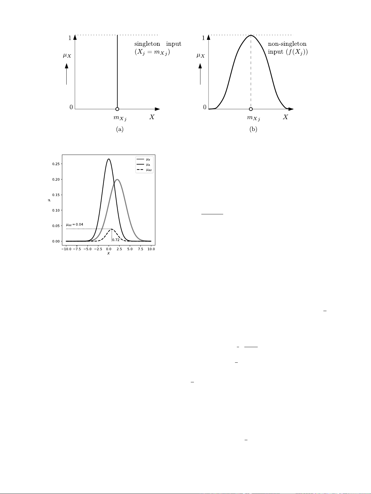
Moreover, an input variable can be singleton [Fig. 2(a)] and non-
singleton [Fig. 2(b)]. Accordingly, a FIS is singleton FIS if it uses
singleton inputs, i.e., FIS uses crisp and precise single value measure-
ments as the input variables, which is the most common practice. How-
ever, real-world problems, especially in engineering, measurements are
noisy, imprecise, and uncertain. Thus, FIS that uses non-singleton input
is a non-singleton FIS. In principle, a non-singleton FIS differs with a
singleton FIS in their respective input fuzzification processes where a
‘‘fuzzifier’’ transform a non-singleton input or a singleton input to a
fuzzy membership value.
A fuzzifier maps a singleton input (crisp input) 𝑋𝑗∈𝐗,𝐗=
(𝑋1, 𝑋2,…, 𝑋𝑃)for 𝑚𝑋𝑗(a value in 𝑋𝑗) [Fig. 2(a)] to the following
membership function for the input fuzzification:
𝜇𝑋𝑗(𝑋𝑗) = {1, 𝑋𝑗=𝑚𝑋𝑗
0, 𝑋𝑖≠𝑚𝑋𝑗∀𝑋𝑗∈𝐗(1)
For non-singleton inputs, a fuzzifier maps input 𝑋𝑗(that is considered
as noisy, imprecise, and uncertain) onto a Gaussian function (typical
choice for numeric variables) as:
𝜇𝑋𝑗(𝑋𝑗) = 𝑓(𝑋𝑗) = exp [−1
2(𝑋𝑗−𝑚𝑋𝑗
𝜎𝑋)2](2)
where 𝑚𝑋𝑗is input (considered as mean, a value along line 𝑋𝑗) and
𝜎𝑋≥0is the standard deviation (std.) that defines the spread of the
function 𝜇𝑋𝑗. The value of the FS at 𝑚𝑋𝑗is 𝜇𝑋𝑗(𝑚𝑋𝑗) = 1 and 𝜇𝑋𝑗(𝑋𝑗)
decreases from unity as 𝑋𝑗moves away from 𝑚𝑋𝑗(Mouzouris and
Mendel,1997). In general, for a singleton or non-singleton input 𝑋𝑗,
the inference engine’s output 𝜇𝐴𝑋𝑗is a combination of fuzzified input
𝜇𝑋𝑗(𝑋𝑗)with an antecedent FS 𝜇𝐴𝑗(𝑋𝑗)as per:
𝜇𝐴𝑋𝑗(
𝑋𝑗) = sup {𝜇𝑋𝑗(𝑋𝑗)⋆ 𝜇𝐴𝑗(𝑋𝑗)}(3)
where ⋆is t-norm operation that can be minimum or product and
𝑋𝑗
indicate supremum of Eq. (3).Fig. 3 is an example of the product
operation in Eq. (3).Fig. 3 evaluates the product of input FS 𝜇𝑋and
the antecedent fuzzy set 𝜇𝐴that results in 𝜇𝐴𝑋 = 0.04 where 𝑚𝑋𝑗= 2.0,
𝜎𝑋= 2.0,𝑚𝐴= 0.0, and 𝜎𝐴= 1.5. The product 𝜇𝐴𝑋 (
𝑋)gives a maximum
value at
𝑋= 0.72 (in Fig. 3) which is calculated as:
𝑋=𝑚𝐴𝜎2
𝑋+𝑚𝑋𝜎2
𝐴
𝜎2
𝐴+𝜎2
𝑋
(4)
The design of RB further distinguishes the type of FISs: a Mamdani-
type FIS (Mamdani,1974) or a Takagi–Sugeno–Kang (TSK)-type
FIS (Takagi and Sugeno,1985). A TSK-type FIS differs with a Mamdani-
type FIS only in the implementation of fuzzy rule’s consequent part.
In Mamdani-type FIS, a rule’s consequent part is an FS, whereas, in
TSK-type FIS, a rule’s consequent part is a polynomial function.
The DB contains the FSs which are either type-1 fuzzy sets (T1FS)
or type-2 fuzzy sets (T2FS). Morover, the FSs are defined using a fuzzy
membership functions (MF) and the basic form of which is coined as
a T1FS. Whereas, T2FS allows an MF to be fuzzy itself by extending
membership value into an additional membership dimension. Hence,
the fuzzy set (FS) types also differentiate FIS types: type-1 FIS (T1FIS)
and the type-2 FIS (T2FIS).
For simplicity, this paper is singleton FIS centric and refers non-
singleton FIS to the appropriate research. As well as, since Mamdani-
type FIS differs with TSK-type FIS only in its consequent part, this paper
focuses on TSK-type FIS.
846
V. Ojha, A. Abraham and V. Snášel Engineering Applications of Artificial Intelligence 85 (2019) 845–864
Fig. 2. Input examples: (a) singleton input 𝜇𝑋𝑗(𝑋𝑗)and (b) non-singleton input 𝜇𝑋𝑗(𝑋𝑗) = 𝑓(𝑋𝑗).
Fig. 3. Product (as a t-norm operation) 𝜇𝐴𝑋 of input FS 𝜇𝑋and the antecedent fuzzy
set 𝜇𝐴as per Eq. (3).
2.1. Type-1 fuzzy inference systems
A TSK-type FIS is governed by the ‘‘IF–THEN’’ rule of the form (Tak-
agi and Sugeno,1985):
𝐫𝑖∶IF 𝑋𝑖
1is 𝐴𝑖
1and ⋯and 𝑋𝑖
𝑝𝑖is 𝐴𝑖
𝑝𝑖THEN 𝑌𝑖is 𝐵𝑖,(5)
where 𝐫𝑖is the 𝑖th rule in the FIS’s RB. The 𝑖th rule has 𝐴𝑖as the T1FS,
and 𝐵𝑖as a function of inputs 𝑋𝑖
1, 𝑋𝑖
2,…, 𝑋𝑖
𝑝𝑖that returns a crisp output
𝑌𝑖. At the 𝑖th rule, 𝑝𝑖≤𝑃inputs are selected from 𝑃inputs. Note that
𝑝𝑖varies from rule-to-rule, and thus, the input dimension at a rule 𝑖is
denoted as 𝑝𝑖. That is, the subset of inputs to a rule has 𝑝𝑖≤𝑃elements,
which leads to a incomplete rule because all available inputs may not be
present to rule premises (antecedent part). Otherwise, a complete rule
has all available inputs at its premises. The function 𝐵𝑖, for TSK-type,
is commonly expressed as:
𝐵𝑖=𝑐𝑖
0+
𝑝𝑖
∑
𝑗=1
𝑐𝑖
𝑗𝑋𝑖
𝑗,(6)
where 𝑋𝑖
𝑗are the inputs and 𝑐𝑖
𝑗for 𝑗= 0 to 𝑝𝑖are the tuneable
parameters at the consequent part of a rule. For Mamdani-type, 𝐵𝑖may
be expressed as a ‘‘class.’’ The basic building blocks of a FIS is shown in
Fig. 1 whose defuzzified crisp output is computed as follows. At first,
the inference engine fires the RB’s rules, each rule has a firing strength
𝐹𝑖as:
𝐹𝑖=
𝑝𝑖
∏
𝑗=1
𝜇𝐴𝑖
𝑗(𝑋𝑖
𝑗),(7)
where 𝜇𝐴𝑖
𝑗∈ [0,1] is the membership value of 𝑗th T1FS MF (e.g.,
Fig. 4(a)) at the 𝑖th rule. Assuming firing strength 𝐹𝑖has to be computed
for a non-singleton input 𝜇𝑋𝑖
𝑗(𝑋𝑖
𝑗), then firing strength 𝐹𝑖will replace
𝜇𝐴𝑖
𝑗(𝑋𝑖
𝑗)in Eq. (7) by 𝜇𝐴𝑋𝑖
𝑗(𝑋𝑖
𝑗)as per Eq. (3). A detail generalize
definition of firing strength computation for non-singleton inputs is
given by Mouzouris and Mendel (1997).
The defuzzified output
𝑌of T1FIS, as an example, is computed as:
𝑌=∑𝑀
𝑖=1 𝐵𝑖𝐹𝑖
∑𝑀
𝑖=1 𝐹𝑖,(8)
where 𝑀is the total rules in the RB.
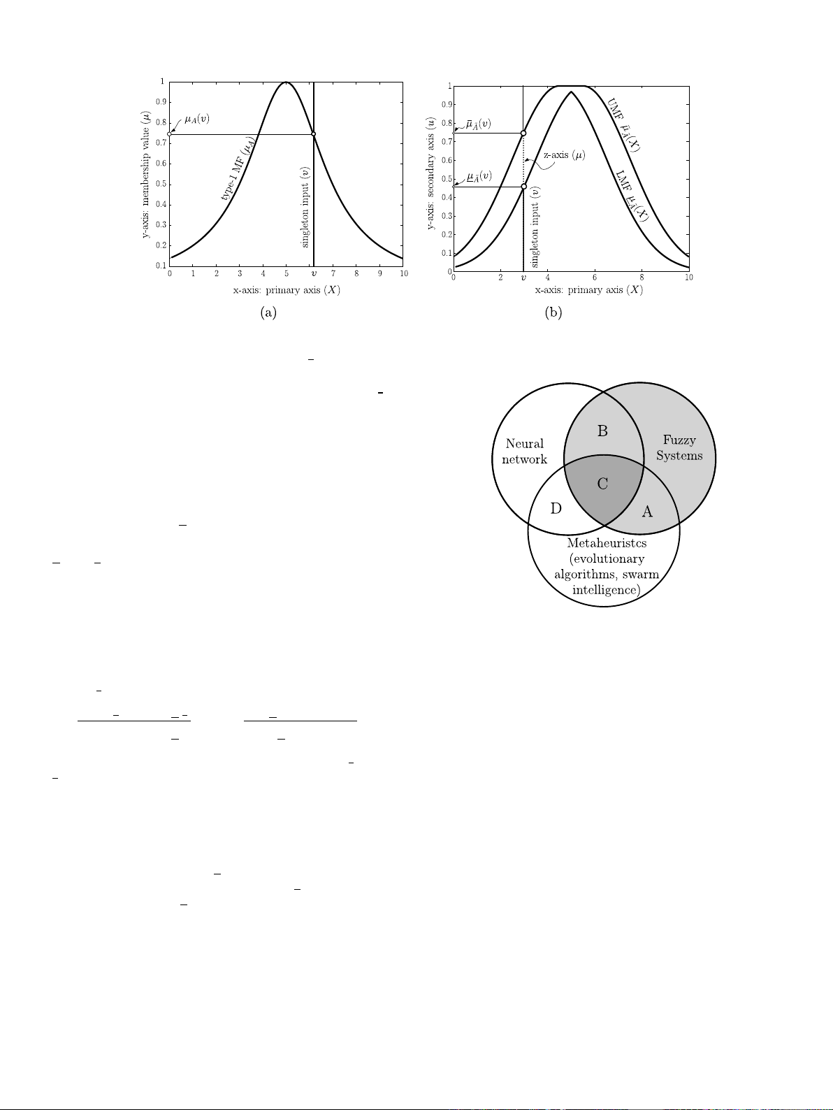
2.2. Type-2 fuzzy inference systems
A T2FS
𝐴is characterized by a 3D MF (Mendel,2013): The 𝑥-axis
is the primary variable, the 𝑦-axis is secondary variable (primary MF
denoted by 𝑢), and the 𝑧-axis is the MF value (secondary MF denoted
by 𝜇). Hence, for a singleton input 𝑋, a T2FS
𝐴is defined as:
𝐴={((𝑋, 𝑢), 𝜇
𝐴(𝑋, 𝑢))|∀𝑋∈𝐗,∀𝑢∈ [0,1]}.(9)
The MF value 𝜇has a 2D support, called ‘‘footprint of uncertainty’’ of
𝐴, which is bounded a lower membership function (LMF) 𝜇
𝐴(𝑋)and
an upper membership function (UMF) 𝜇
𝐴(𝑋). A T2FS bounded by an
LMF and a UMF is an interval type-2 fuzzy set (IT2FS), e.g., a Gaussian
function [Eq. (10)] with uncertain mean 𝑚∈ [𝑚1, 𝑚2]and std. 𝜎≥0is
an IT2FS (e.g., Fig. 4(b)):
𝜇
𝐴(𝑋, 𝑚, 𝜎) = exp (−1
2(𝑋−𝑚
𝜎)2), 𝑚 ∈ [𝑚1, 𝑚2].(10)
An LMF [Eq. (11)]𝜇
𝐴(𝑋) ∈ [0,1] and a UMF [Eq. (12)]𝜇
𝐴(𝑋) ∈ [0,1]
of an IT2FS can be defined as (Karnik et al.,1999):
𝜇
𝐴(𝑋) = {𝜇
𝐴(𝑋, 𝑚2, 𝜎), 𝑋 ≤(𝑚1+𝑚2)∕2
𝜇
𝐴(𝑋, 𝑚1, 𝜎), 𝑋 > (𝑚1+𝑚2)∕2 (11)
𝜇
𝐴(𝑋) = ⎧
⎪
⎨
⎪
⎩
𝜇
𝐴(𝑋, 𝑚1, 𝜎), 𝑋 < 𝑚1
1, 𝑚1≤𝑥≤𝑚2
𝜇
𝐴(𝑋, 𝑚2, 𝜎), 𝑋 > 𝑚2
(12)
In Fig. 4(b), a point 𝑣along the 𝑥-axis of 3D-IT2FS cuts the UMF and
LMF along the 𝑦-axis, and the value 𝜇of the type-2 MF is taken along
the 𝑧-axis [dotted line, which a MF in the third dimension in Fig. 4(b)
between 𝜇
𝐴(𝑋=𝑣)and 𝜇
𝐴(𝑋=𝑣)]. Considering the IT2FS MF, the 𝑖th
IF–THEN rule of TSK-type T2FIS, for inputs 𝐗= (𝑋1, 𝑋2,…, 𝑋𝑝𝑖), takes
the form:
𝐫𝑖∶IF 𝑋𝑖
1is
𝐴𝑖
1and ⋯and 𝑋𝑖
𝑝𝑖is
𝐴𝑖
𝑝𝑖THEN 𝑌𝑖is
𝐵𝑖,(13)
847
V. Ojha, A. Abraham and V. Snášel Engineering Applications of Artificial Intelligence 85 (2019) 845–864
Fig. 4. Fuzzy MF examples: (a) Type-1 MF 𝜇𝐴(𝑋) = 1∕[1 + ((𝑋−𝑚)∕𝜎)2]with center 𝑚= 5.0and width 𝜎= 2.0. (b)Type-2 MF with fixed 𝜎= 2.0and with means 𝑚1= 4.5and
𝑚2= 5.5. UMF 𝜇
𝐴(𝑋)as per Eq. (12) is in solid line and LMF 𝜇
𝐴(𝑋)as per Eq. (11) is in dotted line.
where
𝐴𝑖is a T2FS,
𝐵𝑖is a function of 𝐗that returns a pair [𝑏𝑖,
𝑏𝑖]
called left and right weights of the consequent part of a rule. In TSK,
𝐵𝑖is usually written as:
𝐵𝑖= [𝑐𝑖
0−𝑠𝑖
0, 𝑐𝑖
0+𝑠𝑖
0] +
𝑝𝑖
∑
𝑗=1
[𝑐𝑖
𝑗−𝑠𝑖
𝑗, 𝑐𝑖
𝑗+𝑠𝑖
𝑗]𝑋𝑖
𝑗,(14)
where 𝑋𝑖
𝑗are the inputs and 𝑐𝑖
𝑗for 𝑗= 0 to 𝑝𝑖are the rule’s consequent
part’s tunable parameters and 𝑠𝑖
𝑗for 𝑗= 0 to 𝑝𝑖are its deviation factors.
The firing strength 𝐹𝑖= [𝑓𝑖,
𝑓𝑖]of IT2FS is computed as:
𝑓𝑖=
𝑝𝑖
∏
𝑗
𝜇
𝐴𝑖
𝑗
and
𝑓𝑖=
𝑝𝑖
∏
𝑗
𝜇
𝐴𝑖
𝑗.(15)
At this stage, the inference engine fires the rule and the type-reducer,
e.g., center of set 𝑌𝑐𝑜𝑠 as per Eq. (16) reduces the T2FS to T1FS (Karnik
et al.,1999;Wu and Mendel,2009):
𝑌𝑐𝑜𝑠 = [𝑌𝑙, 𝑌𝑟](16)
where 𝑌𝑙and 𝑌𝑟are left and right ends of the interval. For the ascending
order of 𝑏𝑖and
𝑏𝑖,𝑦𝑙and 𝑦𝑟are computed as:
𝑌𝑙=∑𝐿
𝑖=1
𝑓𝑖𝑏𝑖+∑𝑀
𝑖=𝐿+1 𝑓𝑖𝑏𝑖
∑𝐿
𝑖=1
𝑓𝑖+∑𝑀
𝑖=𝐿+1 𝑓𝑖and 𝑌𝑟=∑𝑅
𝑖=1 𝑓𝑖
𝑏𝑖+∑𝑀
𝑖=𝑅+1
𝑓𝑖
𝑏𝑖
∑𝑅
𝑖=1 𝑓𝑖+∑𝑀
𝑖=𝑅+1
𝑓𝑖,(17)
where 𝐿and 𝑅are the switch points determined as per 𝑏𝐿≤𝑌𝑙≤
𝑏𝐿+1 and
𝑏𝑅≤𝑌𝑟≤
𝑏𝑅+1, respectively. Subsequently, defuzzified crisp
output
𝑌= (𝑌𝑙+𝑌𝑟)∕2 is computed.
For a non-singleton interval type-2 FIS, lower and upper intervals
of non-singleton inputs are created. Additionally, similar to the non-
singleton input fuzzification 𝜇𝐴𝑋 in the case of non-singleton type-1
FIS using input FS 𝜇𝑋and antecedent FS 𝜇𝐴shown in Eq. (3), for non-
singleton type-2 FIS, both lower 𝜇
𝐴𝑋 and upper 𝜇
𝐴𝑋 intervals products
are calculated using lower and upper input FSs 𝜇𝑋and 𝜇𝑋and lower
and upper antecedent FSs 𝜇
𝐴and 𝜇
𝐴.Sahab and Hagras (2011) describe
the computation of non-singleton type-2 FIS in detail.
2.3. Heuristic designs of fuzzy systems
The FIS types: Type-1 (Section 2.1) and Type-2 (Section 2.2) follow
a similar design procedure and differ only in the type of FSs being
used. The heuristic design of FIS can be viewed from its hybridization
with neural networks (NN), evolutionary algorithms (EA), and meta-
Fig. 5. Spectrum of fuzzy inference system paradigms.
heuristics (MH) (Fig. 5). And, such a confluence offers the following
systems (Herrera,2008):
(1) genetic fuzzy systems (A);
(2) neuro-fuzzy systems (B);
(3) hybrid neuro-genetic fuzzy systems (C); and
(4) heuristics design of NNs (D).
This paper discusses the areas A, B, and C of Fig. 5, and the discussion
on area D of Fig. 5 is offered by Ojha et al. (2017).
The heuristic design installs learning capabilities into FIS which
come from the optimization of its components. The FIS optimiza-
tion/learning in a supervised environment is common practice. Typically,
in supervised learning, a FIS is trained/optimized by supplying train-
ing data (𝐗,𝐘) of 𝑁input–output pairs, i.e., 𝐗= (𝑋1, 𝑋2,…, 𝑋𝑃)and
𝐘= (𝑌1, 𝑌2,…, 𝑋𝑄). Each input variable 𝑋𝑗=⟨𝑥𝑗1, 𝑥𝑗2,…, 𝑥𝑗𝑁 ⟩𝑇is
an 𝑁-dimensional vector, and it has a corresponding 𝑁-dimensional
desired output vector 𝑌𝑗=⟨𝑦𝑗1, 𝑦𝑗2,…, 𝑦𝑗𝑁 ⟩𝑇. For the training data
(𝐗,𝐘), a FIS model 𝑓(𝐗, 𝑅)produces output
𝐘= (
𝑌1,
𝑌2,…,
𝑌𝑄), where
𝑓∶𝐗×𝐘→
𝐘,𝑅= {𝐫1,𝐫2,…,𝐫𝑀}is a set of fuzzy 𝑀rules, and
𝑌𝑗=⟨𝑦𝑗1, 𝑦𝑗2,…, 𝑦𝑗𝑁 ⟩𝑇is an 𝑁-dimensional model’s output, which
is compared with the desired output 𝑌𝑗,∀𝑗= 1,2,…, 𝑄 and ∀𝑘=
1,2,…, 𝑁, by using some error/distance/cost function 𝑐𝑓over model
𝑓(𝐗, 𝑅).
The cost function 𝑐𝑓can be a mean squared error function or
can be an accuracy measure, depending on the desired outputs be-
ing continuous (regression) or discrete (classification) (Caruana and
848
V. Ojha, A. Abraham and V. Snášel Engineering Applications of Artificial Intelligence 85 (2019) 845–864
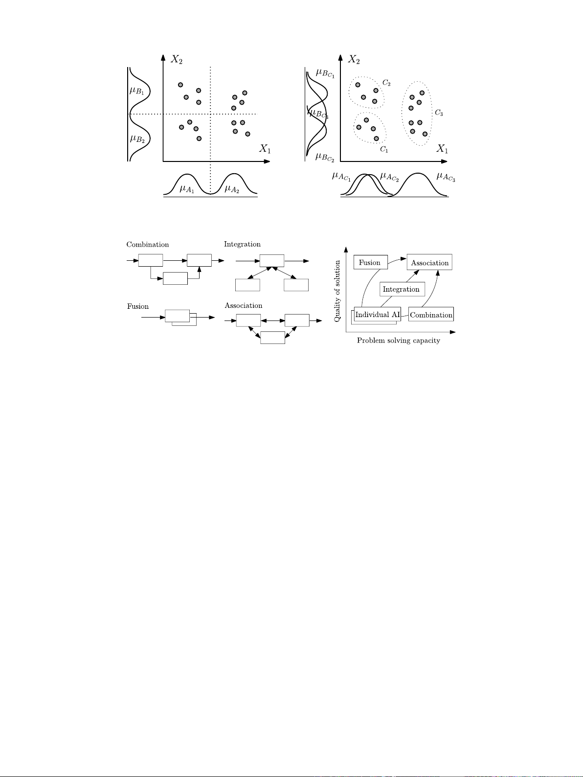
Fig. 6. Input-space partitioning: grid partitioning (left) and clustering partitioning (right). Two-dimensional input-space (inputs 𝑋1and 𝑋2) is partitioned by assigning MF 𝜇𝐴𝑗to
input 𝑋1and MF 𝜇𝐵𝑗to input 𝑋2. In the case of grid partitioning (left), 𝑗= 1,2; and in the case of clustering based partitioning (right), 𝑗=𝐶1, 𝐶2, 𝐶3.
Fig. 7. Synergetic artificial intelligence (Funabashi et al.,1995).
Niculescu-Mizil,2004). FIS’s learning is therefore rely on reducing a
cost function 𝑐𝑓by employing strategies for designing and optimizing
a FIS model 𝑓(𝐗, 𝑅), where model design may be refereed to how the
FIS’s components interact with each other and optimization may be
referred to: RB design, RB parameter learning, and rule selection. In
summary, FIS design, optimization, learning, and modeling is viewed
as:
(1) the selection of FSs via fuzzy partitioning of input-space;
(2) the design of FIS’s rules via an arrangement of rule and inputs;
(3) the optimization of the rule’s parameters; and
(4) the inference from the designed FIS.
Often a Gaussian function, a triangular function, or a trapezoidal
function are selected as the MF of an FS (Zadeh,1999). The input-
space partition corresponding to the MF assignments is one of the
most crucial aspects of FIS design. For example, a two-dimension input-
space in Fig. 6 having inputs 𝑋1and 𝑋2are partitioned using a
grid-partitioning method (Jin,2000;Jang,1993) or a clustering-based
partitioning method (Juang and Lin,1998;Kasabov and Song,2002).
Fig. 6 is an example of inputs space partitioning for numerical
variables. An example of partitioning for linguistic terms is explained
by Cord et al. (2001). Mao et al. (2005) presented an example of input-
space partitioning using a binary tree, where the root of the tree takes
whole input 𝐗and partition it into two children nodes 𝑋𝑙∈𝐗and
𝑋𝑟∈𝐗. The partitioned subsets {𝑋𝑙, 𝑋𝑟}⊂𝐗are assessed for a defined
cost function 𝑐𝑓. If the cost 𝑐𝑓is lower than a defined threshold 𝜖𝑒𝑟𝑟
than the input-space partitioning stops, else continues.
After the input-space partition, FIS is designed via an arrangement
of rules and optimization of rule’s parameters for inference from FIS. As
per Fig. 5, FIS design can be performed by combining the FIS concept
with GA and NN. Such synergy between two or more methods improves
the system’s approximation capabilities (Funabashi et al.,1995). In this
respect, let us revisit four different synergetic models (Fig. 7) which
indicate four ways of hybridizing artificial intelligence (AI) techniques.
The fuzzy system modeling combined with EA, MH, and NN falls in
within the synergetic model: (1) combination, when the produced rules
are optimized by an EA algorithm or an MH algorithm, and (2) fusion,
when EA or an NN are used to design FIS, i.e., to construct RB.
3. Genetic fuzzy systems
EA (Back,1996) and MH (Talbi,2009) have been effective in FIS
optimization (Cordón et al.,2004;Herrera,2008;Sahin et al.,2012).
EA and MH are applied to design, optimize, and learn the fuzzy rules
and this gives the notions of evolutionary/genetic fuzzy systems (GFS)
whose implementational requirements are:
(1) defining a population structure;
(2) encoding FIS’s elements as the individuals in the population;
(3) defining genetic/meta-heuristic operators; and
(4) defining fitness functions relevant to the problem.
3.1. Encoding of genetic fuzzy systems
The questions how to define a population structure and how to en-
code elements of a FIS as the individuals (called chromosome) of the
population opens a diverse implementation of GFS. A FIS has the
following elements: input–output variables; rule’s premises FSs; rule’s
consequent FSs and rule’s parameters; and the rule set. These elements
are combined (encoded to create a vector) in a varied manner that
offers diversity in answering the mentioned questions.
Let 𝑅be an RB, a set of 𝑀rules 𝐫𝑖∈𝑅, ∀𝑖= 1,2,…, 𝑀, then Fig. 8
represent two basic genetic population structures: 𝑎and 𝑏.
A rule 𝐫𝑖∈𝑅that has 𝑝𝑖FSs, 𝐴𝑖for T1FS and
𝐴𝑖for T2FS, for
𝑖= 1 to 𝑝𝑖, the 𝑖th rule parameter vector 𝐫𝑖may be encoded as (Herrera
et al.,1995;Ishibuchi et al.,1997b;Ojha et al.,2016):
𝐫𝑖={⟨𝐴𝑖
1, 𝐴𝑖
2,…, 𝐴𝑖
𝑝𝑖, 𝑐𝑖
0, 𝑐𝑖
1,…, 𝑐𝑖
𝑝𝑖⟩for T1FS
⟨
𝐴𝑖
1,
𝐴𝑖
2,…,
𝐴𝑖
𝑝𝑖, 𝑐𝑖
0, 𝑠𝑖
0, 𝑐𝑖
1, 𝑠𝑖
1,…, 𝑐𝑖
𝑝, 𝑠𝑖
𝑝⟩for T2FS (18)
849


![Bài giảng Mạng nơ-ron nhân tạo trường Đại học Cần Thơ [PDF]](https://cdn.tailieu.vn/images/document/thumbnail/2013/20130331/o0_mrduong_0o/135x160/8661364662930.jpg)