Evolving Artificial Neural Networks
XIN YAO, SENIOR MEMBER, IEEE
Invited Paper
Learning and evolution are two fundamental forms of adapta-
tion. There has been a great interest in combining learning and
evolution with artificial neural networks (ANN’s) in recent years.
This paper: 1) reviews different combinations between ANN’s and
evolutionary algorithms (EA’s), including using EA’s to evolve
ANN connection weights, architectures, learning rules, and input
features; 2) discusses different search operators which have been
used in various EA’s; and 3) points out possible future research
directions. It is shown, through a considerably large literature
review, that combinations between ANN’s and EA’s can lead to
significantly better intelligent systems than relying on ANN’s or
EA’s alone.
Keywords—Evolutionary computation, intelligent systems, neu-
ral networks.
I. INTRODUCTION
Evolutionary artificial neural networks (EANN’s) refer
to a special class of artificial neural networks (ANN’s) in
which evolution is another fundamental form of adaptation
in addition to learning [1]–[5]. Evolutionary algorithms
(EA’s) are used to perform various tasks, such as con-
nection weight training, architecture design, learning rule
adaptation, input feature selection, connection weight ini-
tialization, rule extraction from ANN’s, etc. One distinct
feature of EANN’s is their adaptability to a dynamic
environment. In other words, EANN’s can adapt to an en-
vironment as well as changes in the environment. The two
forms of adaptation, i.e., evolution and learning in EANN’s,
make their adaptation to a dynamic environment much more
effective and efficient. In a broader sense, EANN’s can be
regarded as a general framework for adaptive systems, i.e.,
systems that can change their architectures and learning
rules appropriately without human intervention.
This paper is most concerned with exploring possible
benefits arising from combinations between ANN’s and
EA’s. Emphasis is placed on the design of intelligent
systems based on ANN’s and EA’s. Other combinations
Manuscript received July 10, 1998; revised February 18, 1999. This
work was supported in part by the Australian Research Council through
its small grant scheme.
The author is with the School of Computer Science, University
of Birmingham, Edgbaston, Birmingham B15 2TT U.K. (e-mail:
xin@cs.bham.ac.uk).
Publisher Item Identifier S 0018-9219(99)06906-6.
between ANN’s and EA’s for combinatorial optimization
will be mentioned but not discussed in detail.
A. Artificial Neural Networks
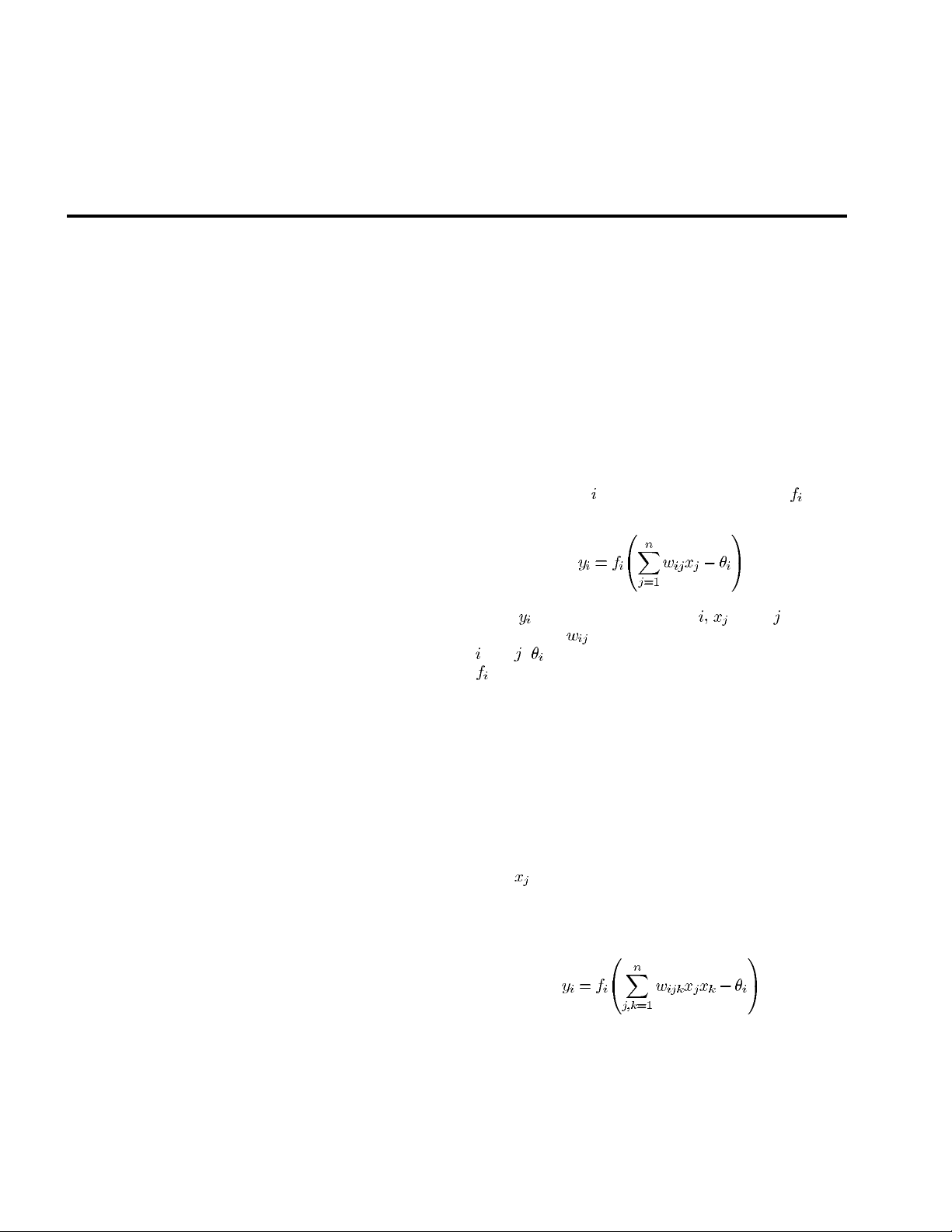
1) Architectures: An ANN consists of a set of processing
elements, also known as neurons or nodes, which are
interconnected. It can be described as a directed graph in
which each node performs a transfer function of the
form
(1)
where is the output of the node is the th input to
the node, and is the connection weight between nodes
and . is the threshold (or bias) of the node. Usually,
is nonlinear, such as a heaviside, sigmoid, or Gaussian
function.
ANN’s can be divided into feedforward and recurrent
classes according to their connectivity. An ANN is feed-
forward if there exists a method which numbers all the
nodes in the network such that there is no connection from
a node with a large number to a node with a smaller number.
All the connections are from nodes with small numbers to
nodes with larger numbers. An ANN is recurrent if such a
numbering method does not exist.
In (1), each term in the summation only involves one
input . High-order ANN’s are those that contain high-
order nodes, i.e., nodes in which more than one input
are involved in some of the terms of the summation. For
example, a second-order node can be described as
where all the symbols have similar definitions to those in
(1).
The architecture of an ANN is determined by its topo-
logical structure, i.e., the overall connectivity and transfer
function of each node in the network.
0018–9219/99$10.00 1999 IEEE
PROCEEDINGS OF THE IEEE, VOL. 87, NO. 9, SEPTEMBER 1999 1423

Fig. 1. A general framework of EA’s.
2) Learning in ANN’s: Learning in ANN’s is typically
accomplished using examples. This is also called “training”
in ANN’s because the learning is achieved by adjusting the
connection weights1in ANN’s iteratively so that trained
(or learned) ANN’s can perform certain tasks. Learning in
ANN’s can roughly be divided into supervised, unsuper-
vised, and reinforcement learning. Supervised learning is
based on direct comparison between the actual output of
an ANN and the desired correct output, also known as the
target output. It is often formulated as the minimization
of an error function such as the total mean square error
between the actual output and the desired output summed
over all available data. A gradient descent-based optimiza-
tion algorithm such as backpropagation (BP) [6] can then
be used to adjust connection weights in the ANN iteratively
in order to minimize the error. Reinforcement learning is a
special case of supervised learning where the exact desired
output is unknown. It is based only on the information of
whether or not the actual output is correct. Unsupervised
learning is solely based on the correlations among input
data. No information on “correct output” is available for
learning.
The essence of a learning algorithm is the learning rule,
i.e., a weight-updating rule which determines how connec-
tion weights are changed. Examples of popular learning
rules include the delta rule, the Hebbian rule, the anti-
Hebbian rule, and the competitive learning rule [7].
More detailed discussion of ANN’s can be found in [7].
B. EA’s
EA’s refer to a class of population-based stochastic
search algorithms that are developed from ideas and princi-
ples of natural evolution. They include evolution strategies
(ES) [8], [9], evolutionary programming (EP) [10], [11],
[12], and genetic algorithms (GA’s) [13], [14]. One im-
portant feature of all these algorithms is their population-
based search strategy. Individuals in a population compete
and exchange information with each other in order to
perform certain tasks. A general framework of EA’s can
be described by Fig. 1.
EA’s are particularly useful for dealing with large com-
plex problems which generate many local optima. They are
less likely to be trapped in local minima than traditional
1Thresholds (biases) can be viewed as connection weights with fixed
input
0
1.
gradient-based search algorithms. They do not depend
on gradient information and thus are quite suitable for
problems where such information is unavailable or very
costly to obtain or estimate. They can even deal with
problems where no explicit and/or exact objective function
is available. These features make them much more robust
than many other search algorithms. Fogel [15] and B¨
ack
et al. [16] give a good introduction to various evolutionary
algorithms for optimization.
C. Evolution in EANN’s
Evolution has been introduced into ANN’s at roughly
three different levels: connection weights; architectures;
and learning rules. The evolution of connection weights
introduces an adaptive and global approach to training,
especially in the reinforcement learning and recurrent net-
work learning paradigm where gradient-based training al-
gorithms often experience great difficulties. The evolution
of architectures enables ANN’s to adapt their topologies
to different tasks without human intervention and thus
provides an approach to automatic ANN design as both
ANN connection weights and structures can be evolved.
The evolution of learning rules can be regarded as a process
of “learning to learn” in ANN’s where the adaptation of
learning rules is achieved through evolution. It can also be
regarded as an adaptive process of automatic discovery of
novel learning rules.
D. Organization of the Article
The remainder of this paper is organized as follows.
Section II discusses the evolution of connection weights.
The aim is to find a near-optimal set of connection weights
globally for an ANN with a fixed architecture using EA’s.
Various methods of encoding connection weights and dif-
ferent search operators used in EA’s will be discussed.
Comparisons between the evolutionary approach and con-
ventional training algorithms, such as BP, will be made.
In general, no single algorithm is an overall winner for all
kinds of networks. The best training algorithm is problem
dependent.
Section III is devoted to the evolution of architectures,
i.e., finding a near-optimal ANN architecture for the tasks
at hand. It is known that the architecture of an ANN
determines the information processing capability of the
ANN. Architecture design has become one of the most
1424 PROCEEDINGS OF THE IEEE, VOL. 87, NO. 9, SEPTEMBER 1999
Fig. 2. A typical cycle of the evolution of connection weights.
important tasks in ANN research and application. Two most
important issues in the evolution of architectures, i.e., the
representation and search operators used in EA’s, will be
addressed in this section. It is shown that evolutionary
algorithms relying on crossover operators do not perform
very well in searching for a near-optimal ANN architecture.
Reasons and empirical results will be given in this section
to explain why this is the case.
If imagining ANN’s connection weights and architectures
as their “hardware,” it is easier to understand the importance
of the evolution of ANN’s “software”—learning rules.
Section IV addresses the evolution of learning rules in
ANN’s and examines the relationship between learning
and evolution, e.g., how learning guides evolution and
how learning itself evolves. It is demonstrated that an
ANN’s learning ability can be improved through evolution.
Although research on this topic is still in its early stages,
further studies will no doubt benefit research in ANN’s and
machine learning as a whole.
Section V summarizes some other forms of combinations
between ANN’s and EA’s. They do not intend to be
exhaustive, simply indicative. They demonstrate the breadth
of possible combinations between ANN’s and EA’s.
Section VI first describes a general framework of
EANN’s in terms of adaptive systems where interactions
among three levels of evolution are considered. The
framework provides a common basis for comparing
different EANN models. The section then gives a brief
summary of the paper and concludes with a few remarks.
II. THE EVOLUTION OF CONNECTION WEIGHTS
Weight training in ANN’s is usually formulated as min-
imization of an error function, such as the mean square
error between target and actual outputs averaged over all
examples, by iteratively adjusting connection weights. Most
training algorithms, such as BP and conjugate gradient
algorithms [7], [17]–[19], are based on gradient descent.
There have been some successful applications of BP in
various areas [20]–[22], but BP has drawbacks due to its use
of gradient descent [23], [24]. It often gets trapped in a local
minimum of the error function and is incapable of finding
a global minimum if the error function is multimodal
and/or nondifferentiable. A detailed review of BP and other
learning algorithms can be found in [7], [17], and [25].
One way to overcome gradient-descent-based training
algorithms’ shortcomings is to adopt EANN’s, i.e., to for-
mulate the training process as the evolution of connection
weights in the environment determined by the architecture
and the learning task. EA’s can then be used effectively
in the evolution to find a near-optimal set of connection
weights globally without computing gradient information.
The fitness of an ANN can be defined according to different
needs. Two important factors which often appear in the
fitness (or error) function are the error between target and
actual outputs and the complexity of the ANN. Unlike
the case in gradient-descent-based training algorithms, the
fitness (or error) function does not have to be differentiable
or even continuous since EA’s do not depend on gradient
information. Because EA’s can treat large, complex, non-
differentiable, and multimodal spaces, which are the typical
case in the real world, considerable research and application
has been conducted on the evolution of connection weights
[24], [26]–[112].
The evolutionary approach to weight training in ANN’s
consists of two major phases. The first phase is to decide
the representation of connection weights, i.e., whether in
the form of binary strings or not. The second one is
the evolutionary process simulated by an EA, in which
search operators such as crossover and mutation have to
be decided in conjunction with the representation scheme.
Different representations and search operators can lead to
quite different training performance. A typical cycle of the
evolution of connection weights is shown in Fig. 2. The
evolution stops when the fitness is greater than a predefined
value (i.e., the training error is smaller than a certain value)
or the population has converged.
A. Binary Representation
The canonical genetic algorithm (GA) [13], [14] has
always used binary strings to encode alternative solutions,
often termed chromosomes. Some of the early work in
evolving ANN connection weights followed this approach
YAO: EVOLVING ARTIFICIAL NEURAL NETWORKS 1425
(a) (b)
Fig. 3. (a) An ANN with connection weights shown. (b) A
binary representation of the weights, assuming that each weight
is represented by four bits.
[24], [26], [28], [37], [38], [41], [52], [53]. In such a repre-
sentation scheme, each connection weight is represented by
a number of bits with certain length. An ANN is encoded by
concatenation of all the connection weights of the network
in the chromosome.
A heuristic concerning the order of the concatenation
is to put connection weights to the same hidden/output
node together. Hidden nodes in ANN’s are in essence
feature extractors and detectors. Separating inputs to the
same hidden node far apart in the binary representation
would increase the difficulty of constructing useful feature
detectors because they might be destroyed by crossover
operators. It is generally very difficult to apply crossover
operators in evolving connection weights since they tend
to destroy feature detectors found during the evolutionary
process.
Fig. 3 gives an example of the binary representation of
an ANN whose architecture is predefined. Each connection
weight in the ANN is represented by 4 bits, the whole ANN
is represented by 24 bits where weight 0000 indicates no
connection between two nodes.
The advantages of the binary representation lie in its
simplicity and generality. It is straightforward to apply
classical crossover (such as one-point or uniform crossover)
and mutation to binary strings. There is little need to design
complex and tailored search operators. The binary repre-
sentation also facilitates digital hardware implementation
of ANN’s since weights have to be represented in terms of
bits in hardware with limited precision.
There are several encoding methods, such as uniform,
Gray, exponential, etc., that can be used in the binary
representation. They encode real values using different
ranges and precisions given the same number of bits.
However, a tradeoff between representation precision and
the length of chromosome often has to be made. If too
few bits are used to represent each connection weight,
training might fail because some combinations of real-
valued connection weights cannot be approximated with
sufficient accuracy by discrete values. On the other hand,
if too many bits are used, chromosomes representing large
ANN’s will become extremely long and the evolution in
turn will become very inefficient.
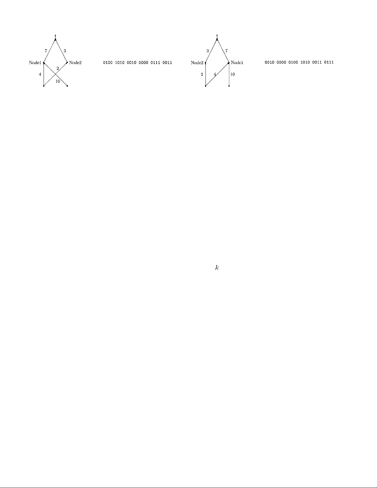
One of the problems faced by evolutionary training of
ANN’s is the permutation problem [32], [113], also known
as the competing convention problem. It is caused by the
(a) (b)
Fig. 4. (a) An ANN which is equivalent to that given in Fig. 3(a).
(b) Its binary representation under the same representation scheme.
many-to-one mapping from the representation (genotype)
to the actual ANN (phenotype) since two ANN’s that order
their hidden nodes differently in their chromosomes will
still be equivalent functionally. For example, ANN’s shown
by Figs. 3(a) and 4(a) are equivalent functionally, but they
have different chromosomes as shown by Figs. 3(b) and
4(b). In general, any permutation of the hidden nodes
will produce functionally equivalent ANN’s with differ-
ent chromosome representations. The permutation problem
makes crossover operator very inefficient and ineffective in
producing good offspring.
B. Real-Number Representation
There have been some debates on the cardinality of
the genotype alphabet. Some have argued that the mini-
mal cardinality, i.e., the binary representation, might not
be the best [48], [114]. Formal analysis of nonstandard
representations and operators based on the concept of
equivalent classes [115], [116] has given representations
other than ary strings a more solid theoretical foundation.
Real numbers have been proposed to represent connection
weights directly, i.e., one real number per connection
weight [27], [29], [30], [48], [63]–[65], [74], [95], [96],
[102], [110], [111], [117], [118]. For example, a real-
number representation of the ANN given by Fig. 3(a) could
be (4.0,10.0,2.0,0.0,7.0,3.0).
As connection weights are represented by real numbers,
each individual in an evolving population will be a real
vector. Traditional binary crossover and mutation can no
longer be used directly. Special search operators have
to be designed. Montana and Davis [27] defined a large
number of tailored genetic operators which incorporated
many heuristics about training ANN’s. The idea was to
retain useful feature detectors formed around hidden nodes
during evolution. Their results showed that the evolutionary
training approach was much faster than BP for the problems
they considered. Bartlett and Downs [30] also demonstrated
that the evolutionary approach was faster and had better
scalability than BP.
A natural way to evolve real vectors would be to use
EP or ES since they are particularly well-suited for treating
continuous optimization. Unlike GA’s, the primary search
operator in EP and ES is mutation. One of the major
advantages of using mutation-based EA’s is that they can
reduce the negative impact of the permutation problem.
Hence the evolutionary process can be more efficient. There
1426 PROCEEDINGS OF THE IEEE, VOL. 87, NO. 9, SEPTEMBER 1999
have been a number of successful examples of applying EP
or ES to the evolution of ANN connection weights [29],
[63]–[65], [67], [68], [95], [96], [102], [106], [111], [117],
[119], [120]. In these examples, the primary search operator
has been Gaussian mutation. Other mutation operators, such
as Cauchy mutation [121], [122], can also be used. EP
and ES also allow self adaptation of strategy parameters.
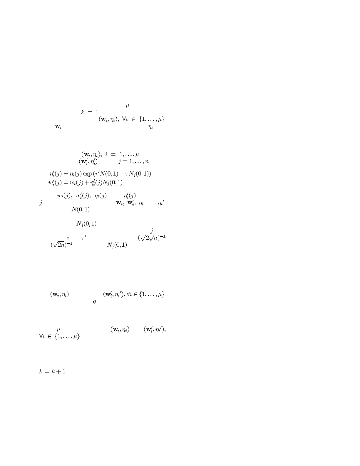
Evolving connection weights by EP can be implemented
as follows.
1) Generate an initial population of individuals at
random and set . Each individual is a pair
of real-valued vectors, ,
where ’s are connection weight vectors and ’s are
variance vectors for Gaussian mutations (also known
as strategy parameters in self-adaptive EA’s). Each
individual corresponds to an ANN.
2) Each individual , creates a
single offspring by: for
(2)
(3)
where , and denote the
th component of the vectors and ,
respectively. denotes a normally distributed
one-dimensional random number with mean zero and
variance one. indicates that the random
number is generated anew for each value of . The
parameters and are commonly set to
and [15], [123]. in (3) may be
replaced by Cauchy mutation [121], [122], [124] for
faster evolution.
3) Determine the fitness of every individual, including
all parents and offspring, based on the training error.
Different error functions may be used here.
4) Conduct pairwise comparison over the union of par-
ents and offspring .
For each individual, opponents are chosen uni-
formly at random from all the parents and offspring.
For each comparison, if the individual’s fitness is
no smaller than the opponent’s, it receives a “win.”
Select individuals out of and
, that have most wins to form the
next generation. (This tournament selection scheme
may be replaced by other selection schemes, such as
[125].)
5) Stop if the halting criterion is satisfied; otherwise,
and go to Step 2).
C. Comparison Between Evolutionary Training
and Gradient-Based Training
As indicated at the beginning of Section II, the evolu-
tionary training approach is attractive because it can handle
the global search problem better in a vast, complex, mul-
timodal, and nondifferentiable surface. It does not depend
on gradient information of the error (or fitness) function
and thus is particularly appealing when this information
is unavailable or very costly to obtain or estimate. For
example, the evolutionary approach has been used to train
recurrent ANN’s [41], [60], [65], [100], [102], [103], [106],
[117], [126]–[128], higher order ANN’s [52], [53], and
fuzzy ANN’s [76], [77], [129], [130]. Moreover, the same
EA can be used to train many different networks regardless
of whether they are feedforward, recurrent, or higher order
ANN’s. The general applicability of the evolutionary ap-
proach saves a lot of human efforts in developing different
training algorithms for different types of ANN’s.
The evolutionary approach also makes it easier to gener-
ate ANN’s with some special characteristics. For example,
the ANN’s complexity can be decreased and its generaliza-
tion increased by including a complexity (regularization)
term in the fitness function. Unlike the case in gradient-
based training, this term does not need to be differentiable
or even continuous. Weight sharing and weight decay can
also be incorporated into the fitness function easily.
Evolutionary training can be slow for some problems in
comparison with fast variants of BP [131] and conjugate
gradient algorithms [19], [132]. However, EA’s are gen-
erally much less sensitive to initial conditions of training.
They always search for a globally optimal solution, while
a gradient descent algorithm can only find a local optimum
in a neighborhood of the initial solution.
For some problems, evolutionary training can be signif-
icantly faster and more reliable than BP [30], [34], [40],
[63], [83], [89]. Prados [34] described a GA-based training
algorithm which is “significantly faster than methods that
use the generalized delta rule (GDR).” For the three tests
reported in his paper [34], the GA-based training algorithm
“took a total of about 3 hours and 20 minutes, and the GDR
took a total of about 23 hours and 40 minutes.” Bartlett and
Downs [30] also gave a modified GA which was “an order
of magnitude” faster than BP for the 7-bit parity problem.
The modified GA seemed to have better scalability than
BP since it was “around twice” as slow as BP for the
XOR problem but faster than BP for the larger 7-bit parity
problem.
Interestingly, quite different results were reported by Ki-
tano [133]. He found that the GA–BP method, a technique
that runs a GA first and then BP, “is, at best, equally
efficient to faster variants of back propagation in very small
scale networks, but far less efficient in larger networks.”
The test problems he used included the XOR problem,
various size encoder/decoder problems, and the two-spiral
problem. However, there have been many other papers
which report excellent results using hybrid evolutionary and
gradient descent algorithms [32], [67], [70], [71], [74], [80],
[81], [86], [103], [105], [110]–[112].
The discrepancy between two seemingly contradictory
results can be attributed at least partly to the different
EA’s and BP compared. That is, whether the comparison
is between a classical binary GA and a fast BP algorithm,
or between a fast EA and a classical BP algorithm. The
discrepancy also shows that there is no clear winner in
terms of the best training algorithm. The best one is always
problem dependent. This is certainly true according to the
YAO: EVOLVING ARTIFICIAL NEURAL NETWORKS 1427


![Bài giảng Mạng nơ-ron nhân tạo trường Đại học Cần Thơ [PDF]](https://cdn.tailieu.vn/images/document/thumbnail/2013/20130331/o0_mrduong_0o/135x160/8661364662930.jpg)