Prediction
of
genetic
merit
from
data
on
binary
and
quantitative
variates
with
an
application
to
calving
difficulty,
birth
weight
and
pelvic
opening
J.L.
FOULLEY,
D.
GIANOLA
R.
THOMPSON’
LN.R.A.,
Station
de
Genetique
quantitative
et
appliquie,
Centre
de
Recherches
zootechniques,
F
78350
Jouy-en-Josas
*
Department
of
Animal
Science,
University
of
Illinois,
Urbana,
Illinois
61801,
U.S.A.,
**
A.R.C.
Unit
of
Statistics,
University
of
Edinburgh,
Mayfield
Road,
Edinburgh,
EH9 3JZ,
Scotland
Summary
A
method
of
prediction
of
genetic
merit
from
jointly
distributed
quanta]
and
quantitative
responses
is
described.
The
probability
of
response
in
one
of
two
mutually
exclusive
and
exhaustive
categories
is
modeled
as
a
non-linear
function
of
classification
and
« risk
» variables.
Inferences
are
made
from
the
mode
of
a
posterior
distribution
resulting
from
the
combination
of
a
multivariate
normal
density,
a
priori,
and
a
product
binomial
likelihood
function.
Parameter
estimates
are
obtained
with
the
Newton-Raphson
algorithm,
which
yields
a
system
similar
to
the
mixed
model
equations.
« Nested
» Gauss-Seidel
and
conjugate
gradient
procedures
are
suggested
to
proceed
from
one
iterate
to
the
next
in
large
problems.
A
possible
method
for
estimating
multivariate
variance
(covariance)
components
involving,
jointly,
the
categorical
and
quantitative
variates
is
presented.
The
method
was
applied
to
prediction
of
calving
difficulty
as
a
binary
variable
with
birth
weight
and
pelvic
opening
as
«
risk
»
variables
in
a
Blonde
d’Aquitaine
population.
Key-words :
sire
evaluation,
categorical
data,
non-linear
models,
prediction,
Bayesian
methods.
Résumé
Prédiction
génétique
à
partir
de
données
binaires
et
continues :
application
aux
difficultés
de
vêlage,
poids
à
la
naissance
et
ouverture
pelvienne.
Cet
article
présente
une
méthode
de
prédiction
de
la
valeur
génétique
à
partir
d’observations
quantitatives
et
qualitatives.
La
probabilité
de
réponse
selon
l’une
des
deux
modalités
exclusives
et
exhaustives
envisagées
est
exprimée
comme
une
fonction
non
linéaire
d’effets
de
facteurs
d’incidence
et
de
variables
de
risque.
L’inférence
statistique
repose
sur
le
mode
de
la
distribution
a
posteriori
qui
combine
une
densité
multinormale
a
priori
et
une
fonction
de
vraisemblance
produit
de
binomiales.
Les
estimations
sont
calculées
à
partir
de
l’algorithme
de
Newton-Raphson
qui
conduit
à
un
système
d’équations
similaires
à
celles
du
modèle
mixte.
Pour
les
gros
fichiers,
on
suggère
des
méthodes
itératives
de
résolution
telles
que
celles
de
Gauss-Seidel
et
du
gradient
conjugué.
On
pro-
pose
également
une
méthode
d’estimation
des
composantes
de
variances
et
covariances
relatives
aux
variables
discrètes
et
continues.
Enfin,
la
méthodologie
présentée
est
illustrée
par
une
application
numérique
qui
a
trait
à
la
prédiction
des
difficultés
de
vêlage
en
race
bovine
Blonde
d’Aquitaine
utilisant
d’une
part,
l’appréciation
tout-ou-rien
du
caractère,
et
d’autre
part,
le
poids
à
la
naissance
du
veau
et
l’ouverture
pelvienne
de
la
mère
comme
des
variables
de
risque.
Mots-clés :
Évaluation
des
reproducteurs,
données
discrètes,
modèle
non
linéaire,
prédiction,
méthode
bayesienne.
1.
Introduction
In
many
animal
breeding
applications,
the
data
comprise
observations
on
one
or
more
quantitative
variates
and
on
categorical
responses.
The
probability
of
«
successful
»
outcome
of
the
discrete
variate,
e.g.,
survival,
may
be
a
non-linear
function
of
genetic
and
non-genetic
variables
(sire,
breed,
herd-year)
and
may
also
depend
on
quantitative
response
variates.
A
possible
course
of
action
in
the
analysis
of
this
type
of
data
might
be
to
carry
out
a
multiple-trait
evaluation
regarding
the
discrete
trait
as
if
it
were
continuous,
and
then
utilizing
available
linear
methodology
(H
ENDER
SO
N,
1973).
Further,
the
model
for
the
discrete
trait
should
allow
for
the
effects
of
the
quantitative
variates.
In
addition
to
the
problems
of
describing
discrete
variation
with
linear
models
(Cox,
1970;
THO
MPSON
,
1979;
G
IANOLA
,
1980),
the
presence
of
stochastic
« regressors
in
the
model
introduces
a
complexity
which
animal
breeding
theory
has
not
addressed.
This
paper
describes
a
method
of
analysis
for
this
type
of
data
based
on
a
Bayesian
approach;
hence,
the
distinction
between
« fixed
and
« random
variables
is
circumvented.
General
aspects
of
the
method
of
inference
are
described
in
detail
to
facilitate
comprehension
of
subsequent
developments.
An
estimation
algorithm
is
developed,
and
we
consider
some
approximations
for
posterior
inference
and
fit
of
the
model.
A
method
is
proposed
to
estimate
jointly
the
components
of
variance
and
covariance
involving
the
quantitative
and
the
categorical
variates.
Finally,
procedures
are
illustrated
with
a
data
set
pertaining
to
calving
difficulty
(categorical),
birth
weight
and
pelvic
opening.
II.
Method
of
inference :
general
aspects
Suppose
the
available
data
pertain
to
three
random
variables:
two
quantitative
(e.g.,
calf’s
birth
weight
and
dam’s
pelvic
opening)
and
one
binary
(e.g.,
easy
vs.
difficult
calving).
Let
the
data
for
birth
weight
and
dam’s
pelvic
opening
be
represented
by
the
vectors
y,
and
Y2
,
respectively.
Those
for
calving
difficulty
are
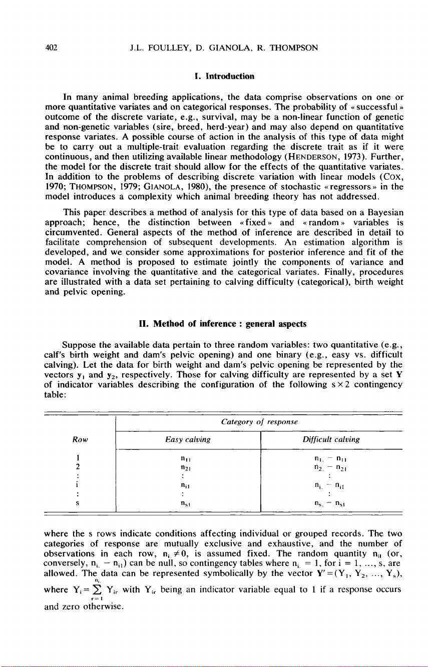
represented
by
a
set
Y
of
indicator
variables
describing
the
configuration
of
the
following
s x
2 contingency
table:
where
the
s
rows
indicate
conditions
affecting
individual
or
grouped
records.
The
two
categories
of
response
are
mutually
exclusive
and
exhaustive,
and
the
number
of
observations
in
each
row,
n; !0,
is
assumed
fixed.
The
random
quantity
n
il
(or,
conversely,
n;
-
ni
,)
can
be
null,
so
contingency
tables
where
n,
=
1,
for
i
=
1,
...,
s,
are
allowed.
The
data
can
be
represented
symbolically
by
the
vector
Y’=(Y,,
Y2,
...,
Y,),
n!,
where
y
i=
7-
Y
ir
with
Yi,
being
an
indicator
variable
equal
to
1
if
a
response
occurs
r=i
I
and
zero
otherwise.
The
data
Y,
y,
and
y2,
and
a
parameter
vector
0
are
assumed
to
have
a
joint
density
f(Y,
y,,
y2,
0)
written
as
where
f,(9)
is
the
marginal
or
a
priori
density
of
0.
From
(1)
where
f3
(Y,
y,
y,)
is
the
marginal
density
of
the
data,
i.e.,
with
0
integrated
out,
and
f4
(o I Y, ,
Y
&dquo;
Y2
)
is
the
a
posteriori
density
of
0.
As
f3
(Y,
y,,
Y2
)
does
not
depend
on
0,
one
can
write
(2)
as
which
is
Bayes
theorem
in
the
context
of
our
setting.
Equation
(3)
states
that
inferences
can
be
made
a
posteriori
by
combining
prior
information
with
data
translated
to
the
posterior
density
via
the
likelihood
function
f2
(Y,
YI
,
Y210).
The
dispersion
of
0
reflects
the
a
priori
relative
uncertainty
about
0,
this
based
on
the
results
of
previous
data
or
experiments.
If
a
new
experiment
is
conducted,
new
data
are
combined
with
the
prior
density
to
yield
the
posterior.
In
turn,
this
becomes
the
a
priori
density
for
further
experiments.
In
this
form,
continued
iteration
with
(3)
illustrates
the
process
of
knowledge
accumulation
(CORNFIELD,
1969).
Comprehensive
discussions
of
the
merits,
philosophy
and
limitations
of
Bayesian
inference
have
been
presented
by
C
ORNFIELD
(1969),
and
LirrDLEY
&
SMITH
(1972).
The
latter
argued
in
the
context
of
linear
models
that
(3)
leads
to
estimates
which
may
be
substantially
improved
from
those
arising
in
the
method
of
least-squares.
Equation
(3)
is
taken
in this
paper
as
a
point
of
departure
for
a
method
of
estimation
similar
to
the
one
used
in
early
developments
of
mixed
model
prediction
(H
ENDER
SO
N
et
al.,
1959).
Best
linear
unbiased
predictors
could
also
be
derived
following
Bayesian
considerations
(R6
NNIN
G
EN
,
1971;
D
EMPFLE
,
1977).
The
Bayes
estimator
of
0
is
the
vector
6
minimizing
the
expected
a
posteriori
risk
where
1(6,
0)
is
a
loss
function
(MOOD
&
GR
A
YB
ILL
,
1963).
If
the
loss
is
quadratic
Equating
(6)
to
zero,
yields
Ô=E(9IY,
yi,
yz
).
Note
that
differentiating
(6)
with
respect
to
0
yields
a
positive
number,
i.e.,
0
minimizes
the
expected
posterior
risk,
and
0
is
identical
to
the
best
predictor
of
0
in
the
squared-error
sense
of
H
ENDERSON
(1973).
Unfortunately,
calculating
4
requires
deriving
the
conditional
density
of
0
given
Y,
y,
and
y,,
and
then
computing
the
conditional
expectation.
In
practice,
this
is
difficult
or
impossible
to
execute
as
discussed
by
H
ENDER
S
ON
(1973).
In
view
of
these
difficulties,
L
INDLEY
&
SMITH
(1972)
have
suggested
to
approximate
the
posterior
mean
by
the
mode
of
the
posterior
density;
if
the
posterior
is
unimodal
and
approximately
symmetric,
its
mode
will
be
close
to
the
mean.
HARVIL
LE
(1977)
has
pointed
out,
that
if
an
improper
prior
is
used
in
place
of
the
« true
prior,
the
posterior
mode
has
the
advantage
over
the
posterior
mean,
of
being
less
sensitive
to
the
tails
of
the
posterior
density.
In
(3),
it
is
convenient
to
write
so
the
log
of
the
posterior
density
can
be
written
as
In[f
4
(Ø/Y,
Yt
, y
z
)] =In[f
6(y
ly,,
Yz
, Ø)]+ In [f
s(
Yt
.
Yzl
ø)]+ 1n[f
¡
(Ø)]
+
const.
(8)
III.
Model
A.
Categorical
variate
The
probability
of
response
(e.g.,
easy
calving)
for the
i’!
row
of
the
contingency
table
can
be
written
as
some
cumulative
distribution
function
with
an
argument
peculiar
to
this
row.
Possibilities
(GI
ANOL
A
&
FOULLEY,
1983)
are
the
standard
normal
and
logistic
distribution
functions.
In
the
first
case,
the
probability
of
response
is
where
<1>(.)
and
(D(.)
are
the
density
and
distribution
functions
of
a
standard
normal
variate,
respectively,
and
w;
is
a
location
variable.
In
the
logistic
case,
The
justification
of
(9)
and
(10)
is
that
they
provide
a
liaison
with
the
classical
threshold
model
(D
EMPST
ER
&
LER
NER,
1950;
G
IAN
O
LA
,
1982).
If
an
easy
calving
occurs
whenever
the
realized
value
of
an
underlying
normal
variable,
zw-N(8
;,
1),
is
less
than
a
fixed
threshold
value
t,
we
can
write
for the
i
lh
row
Letting
p.,=t-8
i,
!Li+5
is
the
probit
transformation
used
in
dose-response
relationships
(F
INNEY
,
1952) ;
defining
!L4,=
¡.
t,’
IT /V3,
then
For -5<p.,<5,
the
difference
between
the
left
and
right
hand
sides
of
( l lb)
does
not
exceed
.022,
being
negligible
from
a
practical
point
of
view.
Suppose
that
a
normal
function
is
chosen
to
describe
the
probability
of
response.
Let
y
;3
be
the
underlying
variable,
which
under
the
conditions
of
the
i’
h
row
of
the
contingency
table,
is
modeled
as
where
X:3
and
Z:3
are
known
row
vectors,
JJ3
and
U3
are
unknown
vectors,
and
ei,
is
a
residual.
Likewise,
the
models
for
birth
weight
and
pelvic
opening
are
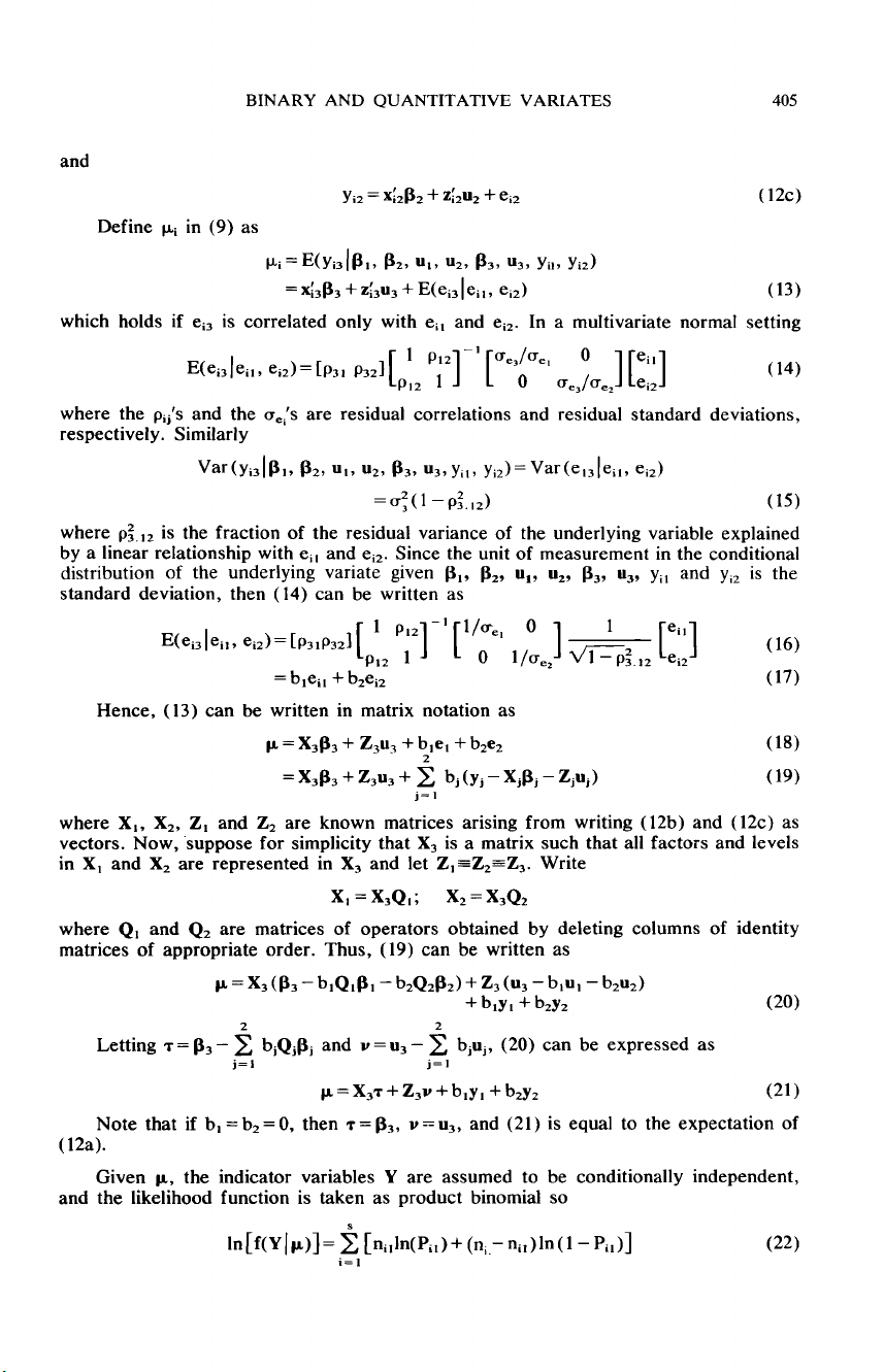
Define
I-Li
in
(9)
as
which
holds
if
e
;3
is
correlated
only
with
ei,
and
e
i2’
In
a
multivariate
normal
setting
where
the
p;
,’s
and
the
(T!,’s
are
residual
correlations
and
residual
standard
deviations,
respectively.
Similarly
where
p! !
is
the
fraction
of
the
residual
variance
of
the
underlying
variable
explained
by
a
linear
relationship
with
e;,
and
e
;2
.
Since
the
unit
of
measurement
in
the
conditional
distribution
of
the
underlying
variate
given
PH
P2
1
Ull
U21
P3
1
u3,
yi,
and
Yi2
is
the
standard
deviation,
then
( 14)
can
be
written
as
Hence,
(13)
can
be
written
in
matrix
notation
as
where
X&dquo;
X2,
Z,
and
Z2
are
known
matrices
arising
from
writing
(12b)
and
(12c)
as
vectors.
Now,
suppose
for
simplicity
that
X3
is
a
matrix
such
that
all
factors
and
levels
in
X,
and
X2
are
represented
in
X3
and
let
ZI =Z
Z
=Z3’
Write
where
Q,
and
Q,
are
matrices
of
operators
obtained
by
deleting
columns
of
identity
matrices
of
appropriate
order.
Thus,
(19)
can
be
written
as
2
2
Letting
T
=
P3 -
L
b
;Q;[
3;
and
v
=
U3 -
L
b,u,,
(20)
can
be
expressed
as
¡-I
i
W
Note
that
if
b, = b
2
= 0,
then
T
= (i
3,
v =
U3
.
and
(21 )
is
equal
to
the
expectation
of
( 12a).
Given
fl
,
the
indicator variables
Y are
assumed
to
be
conditionally
independent,
and
the
likelihood
function
is
taken
as
product
binomial
so


%20--%3e%3cdefs%3e%3cstyle%3e%20.st0%20{%20fill:%20%23fff;%20}%20.st1%20{%20fill:%20%237800fa;%20}%20%3c/style%3e%3c/defs%3e%3cpath%20class='st1'%20d='M117.78,12.18H43.11c2.9,3.47,4.65,7.94,4.65,12.82,0,5.6-2.3,10.66-6.01,14.29h76.02l7.22-13.56-7.22-13.56Z'/%3e%3cg%3e%3cpath%20class='st0'%20d='M53.58,26.17h-.59v-1.46h.59v-4.96h2.83c1.78,0,2.67.94,2.67,2.82v5.76c0,1.87-.89,2.81-2.67,2.81h-2.83v-4.96ZM55.36,21.37v3.34h1.1v1.46h-1.1v3.34h1.01c.61,0,.91-.37.91-1.1v-5.93c0-.74-.3-1.1-.91-1.1h-1.01Z'/%3e%3cpath%20class='st0'%20d='M65.99,31.14h-1.8l-.31-2.07h-2.19l-.31,2.07h-1.64l1.82-11.39h2.62l1.82,11.39ZM65.28,18.04c-.25.46-.51.77-.75.94-.21.15-.47.22-.79.22-.26,0-.57-.07-.92-.22l-.38-.15c-.14-.05-.26-.07-.37-.07-.3,0-.53.18-.71.54l-.91-.68c.25-.46.51-.77.75-.94.21-.14.48-.21.79-.21.26,0,.57.07.92.21l.38.15c.14.05.26.07.37.07.3,0,.53-.18.71-.54l.91.68ZM61.91,27.52h1.73l-.87-5.76-.87,5.76Z'/%3e%3cpath%20class='st0'%20d='M74.53,26.89v1.52c0,1.91-.89,2.86-2.67,2.86s-2.67-.95-2.67-2.86v-5.93c0-1.91.89-2.86,2.67-2.86s2.67.95,2.67,2.86v1.11h-1.69v-1.22c0-.75-.31-1.12-.93-1.12s-.93.37-.93,1.12v6.15c0,.74.31,1.11.93,1.11s.93-.37.93-1.11v-1.63h1.69Z'/%3e%3cpath%20class='st0'%20d='M81.4,31.14h-1.8l-.31-2.07h-2.19l-.31,2.07h-1.64l1.82-11.39h2.62l1.82,11.39ZM75.9,19.2l1.52-1.91h1.71l1.51,1.91h-1.61l-.76-.95-.75.95h-1.61ZM77.32,27.52h1.73l-.87-5.76-.87,5.76ZM83.1,15.99l-1.76,1.91h-1.26l1.17-1.91h1.86Z'/%3e%3cpath%20class='st0'%20d='M84.86,19.75c1.78,0,2.67.94,2.67,2.82v1.48c0,1.87-.89,2.81-2.67,2.81h-.85v4.28h-1.79v-11.39h2.64ZM84.01,21.37v3.86h.85c.58,0,.87-.36.87-1.08v-1.71c0-.71-.29-1.07-.87-1.07h-.85Z'/%3e%3cpath%20class='st0'%20d='M93.51,19.75c1.78,0,2.67.94,2.67,2.82v1.48c0,1.87-.89,2.81-2.67,2.81h-.85v4.28h-1.79v-11.39h2.64ZM92.66,21.37v3.86h.85c.58,0,.87-.36.87-1.08v-1.71c0-.71-.29-1.07-.87-1.07h-.85Z'/%3e%3cpath%20class='st0'%20d='M98.8,31.14h-1.79v-11.39h1.79v4.88h2.03v-4.88h1.83v11.39h-1.83v-4.88h-2.03v4.88Z'/%3e%3cpath%20class='st0'%20d='M105.36,24.55h2.46v1.62h-2.46v3.34h3.09v1.63h-4.88v-11.39h4.88v1.63h-3.09v3.18ZM108.17,17.29l-1.76,1.91h-1.26l1.17-1.91h1.86Z'/%3e%3cpath%20class='st0'%20d='M112.2,19.75c1.78,0,2.67.94,2.67,2.82v1.48c0,1.87-.89,2.81-2.67,2.81h-.85v4.28h-1.79v-11.39h2.64ZM111.35,21.37v3.86h.85c.58,0,.87-.36.87-1.08v-1.71c0-.71-.29-1.07-.87-1.07h-.85Z'/%3e%3c/g%3e%3ccircle%20class='st1'%20cx='25'%20cy='25'%20r='20'/%3e%3cpath%20class='st0'%20d='M32.78,19.27c2.92,0,4.43,2.55,5.28,5.33l.71,2.17c.14.38-.33.75-.71.75h-5.61c.19-.33.24-.71.09-1.08l-.75-2.45c-.43-1.32-.99-2.64-1.79-3.77.75-.57,1.65-.94,2.78-.94h0ZM25,18.38c3.25,0,4.9,2.78,5.89,5.89l.76,2.45c.14.42-.33.8-.8.8h-11.69c-.42,0-.94-.38-.8-.8l.75-2.45c.99-3.11,2.64-5.89,5.89-5.89h0ZM25,11.35c1.74,0,3.11,1.37,3.11,3.11s-1.37,3.11-3.11,3.11-3.11-1.41-3.11-3.11,1.41-3.11,3.11-3.11h0ZM17.27,19.27c1.08,0,1.98.38,2.73.94-.8,1.13-1.37,2.45-1.74,3.77l-.8,2.45c-.14.38-.05.75.09,1.08h-5.56c-.42,0-.9-.38-.75-.75l.71-2.17c.9-2.78,2.41-5.33,5.33-5.33h0ZM17.27,12.91c1.51,0,2.78,1.27,2.78,2.83s-1.27,2.83-2.78,2.83-2.83-1.27-2.83-2.83,1.27-2.83,2.83-2.83h0ZM32.78,12.91c1.56,0,2.78,1.27,2.78,2.83s-1.23,2.83-2.78,2.83-2.83-1.27-2.83-2.83,1.27-2.83,2.83-2.83h0ZM27.07,28.56v.09c0,.57-.24,1.08-.61,1.46h0v.05c-.38.33-.9.57-1.46.57s-1.08-.24-1.46-.61h0c-.38-.38-.61-.9-.61-1.46v-.09h1.41v.09c0,.19.05.38.19.47v.05c.09.09.28.19.47.19s.38-.09.47-.19v-.05c.14-.09.24-.28.24-.47t-.05-.09h1.41ZM30.99,28.56v.09c0,1.65-.66,3.16-1.74,4.24-1.08,1.08-2.59,1.79-4.24,1.79s-3.16-.71-4.24-1.79l-.05-.05c-1.04-1.08-1.7-2.55-1.7-4.2v-.09h1.41v.09c0,1.27.47,2.4,1.27,3.25h.05c.85.85,1.98,1.37,3.25,1.37s2.4-.52,3.25-1.37c.85-.8,1.37-1.98,1.37-3.25v-.09h1.37ZM34.99,28.56v.09c0,2.78-1.13,5.28-2.92,7.07-1.79,1.79-4.29,2.92-7.07,2.92s-5.23-1.13-7.07-2.92c-1.79-1.79-2.92-4.29-2.92-7.07v-.09h1.41v.09c0,2.4.94,4.53,2.5,6.08,1.56,1.56,3.72,2.5,6.08,2.5s4.52-.94,6.08-2.5c1.56-1.56,2.5-3.68,2.5-6.08v-.09h1.41Z'/%3e%3c/svg%3e)