
REGULAR ARTICLE
3D convolutional and recurrent neural networks for reactor
perturbation unfolding and anomaly detection
Aiden Durrant
*
, Georgios Leontidis, and Stefanos Kollias
University of Lincoln, School of Computer Science, Machine Learning Group, Brayford Pool, Lincoln LN6 7TS, UK
Received: 1 July 2019 / Accepted: 12 July 2019
Abstract. With Europe’s ageing fleet of nuclear reactors operating closer to their safety limits, the monitoring
of such reactors through complex models has become of great interest to maintain a high level of availability and
safety. Therefore, we propose an extended Deep Learning framework as part of the CORTEX Horizon 2020 EU
project for the unfolding of reactor transfer functions from induced neutron noise sources. The unfolding allows
for the identification and localisation of reactor core perturbation sources from neutron detector readings in
Pressurised Water Reactors. A 3D Convolutional Neural Network (3D-CNN) and Long Short-Term Memory
(LSTM) Recurrent Neural Network (RNN) have been presented, each to study the signals presented in
frequency and time domain respectively. The proposed approach achieves state-of-the-art results with the
classification of perturbation type in the frequency domain reaching 99.89% accuracy and localisation of the
classified perturbation source being regressed to 0.2902 Mean Absolute Error (MAE).
1 Introduction
The early detection, classification, and localisation of
anomalies within the reactors’core is vital to ensure the
safe and efficient operation of the increasingly aging fleet of
Europe’s reactors. Monitoring of these reactors at nominal
conditions provides vital and valuable insights into the
functional dynamics of the core, consequently allowing for
early identification of anomalies. Analysis of the core
operation is achieved through non-intrusive measuring of
neutron flux around their mean values from in-core and ex-
core detectors. These fluctuations more commonly referred
to as noise are induced primarily from turbulent character-
istics in the coolant flow in the core, coolant boiling, or
mechanical vibrations of reactor’s internal components.
Given detailed descriptions of the reactor core geome-
try, properties of physical perturbations, and probabilities
of neutron interactions, by using a Green’s function as the
reactor transfer function, simulations can be constructed to
show the effect of the neutron noise. Green’s function holds
the relationship between a locally induced perturbation
and the response of the neutron flux within the core,
therefore, the inversion of this function from noise readings
can localise and classify such induced perturbations. This
inversion known as the backwards problem or unfolding is
trivial given measurements at every position within the
core, however, the limited number of in-core and ex-core
detectors makes it a complex challenge [1].
Machine learning (ML) is a data analytical process for
the approximation of functions mapping a set of inputs to
outputs. Therefore, the use of ML to approximate such
reactor functions given limited detector readings is
advantageous, learning high and low-level patterns given
substantial training examples. This work presents an
extended 3D-Convolutional and Recurrent neural network
approach to unfold the reactor transfer function and
classify induced perturbation types and their source
locations in both time and frequency domains.
2 Related work
The application of ML approaches in the field of nuclear
safety has been of recent scientific interest, with nuclear
energy essential to meeting fast changing climate goals.
The ML community has been keen on predicting climate
change [2] utilising a variety of approaches across all energy
sectors. Nuclear energy relies on safety and availability to
achieve such goals, and many recent works have been
proposed to ensure this.
In [3] the authors utilised deep convolutional neural
networks and Naïve-Bayes approaches for vision-based
crack detection for reactor component surfaces from video
sequences. A diagnosis system monitoring the condition of
sensors using auto-associative kernel regression and
sequential probability was proposed in [4]. Deep rectifier
neural networks were implemented in [5] for the accident or
transient scenario identification of pressurised water
reactors (PWR), whereas others solved similar problem
*e-mail: adurrant@lincoln.ac.uk
EPJ Nuclear Sci. Technol. 5, 20 (2019)
©A. Durrant et al., published by EDP Sciences, 2019
https://doi.org/10.1051/epjn/2019047
Nuclear
Sciences
& Technologies
Available online at:
https://www.epj-n.org
This is an Open Access article distributed under the terms of the Creative Commons Attribution License (https://creativecommons.org/licenses/by/4.0),
which permits unrestricted use, distribution, and reproduction in any medium, provided the original work is properly cited.

employing artificial neural networks improving condition-
based maintenance [6]. Further ML approaches were
implemented by [7] in the form of Adaptive Neuro-Fuzzy
Inference System (ANFIS) for the prediction of critical
heat flux. For unfolding, ANFIS approaches have also been
utilised for the localisation of simulated induced neutron
noise sources in VVER-100 rectors, given neutron pulse
height distributions as training input [8,9].
Work proposed in [10] unfolds reactor transfer
functions by the means of CNNs from simulated neutron
noise readings in the frequency domain at differing
perturbation types and frequencies. Classification and
localisation of the perturbations had been achieved with
low error by the means of a 2D-CNN. The localisation of the
perturbation source was achieved through the spatial
splitting of the core volume into 12 and 48 subsections for
classification of source perturbation belonging to a
particular subsection. Furthermore, an increased unfolding
resolution for localisation was implemented, utilising the
extracted latent variables from the CNN and clustering.
Reference [11] proposed a 3D-CNN approach to combat the
limitations of the 2D implementation in [10] from the loss of
spatial information through the conversion of the 3D
volume into a 2D input. Moreover, [11] included the
classification of time domain signals processed to extract
temporal information via RNNs. This work extends the
approaches previously developed in [10,11] to larger, more
complex simulation scenarios, including the localisation of
perturbations in the time domain.
3 Simulated scenarios and data
pre-processing
The process of training ML models requires large amounts
of training data, representing instances for which known
perturbations are assumed and the corresponding induced
neutron noise readings are estimated. The known data
allows the system to learn the function mapping detector
readings to their classification and origin, i.e. transfer
function inversion, or unfolding. To obtain this amount of
training data it is necessary to simulate scenarios to
practically provide enough examples of differing anomaly
types and source locations for effective unfolding. To
achieve this, simulations determining the reactor transfer
function or Green’s function, providing detector readings of
the induced neutron noise of a given perturbation scenarios
for pressurised water reactors (PWR) have been employed
in both the time and frequency domain.
3.1 Frequency domain
Modelling of fluctuations in neutron flux given known
perturbations in the frequency domain was achieved
through the CORE SIM [12] reactor physics codes,
generating neutron detector readings of the induced
neutron noise in a PWR for five perturbation scenarios.
CORE SIM models the effects of a noise source for a three-
dimensional reactor core, of cylindrical shape in Cartesian
geometry for a reactor transfer function considered to be
the Green’s function of the system capturing the
response of the fluctuations of the induced neutron flux
from known perturbation distributions. The Green’s
function provides a one-to-one relationship between any
location of perturbation and the response of the neutron
flux at any position within the core. CORE SIM models a
PWR with a radial core of size 15 15 fuel assemblies,
utilising a fine volumetric mesh of 32 32 34 voxels
modelling sub-assembly response, including boundary
sources. For further details, consult the CORE SIM user
manual [12,13].
CORE SIM provides five perturbations scenarios in 34
frequencies (0.1–1.0 Hz with a step of 0.1 Hz and 1.0–
25.0 Hz with a step of 1.0 Hz) each with two energy
groups, i.e. high and low energy spectrum, referred to as
Fast and Thermal groups respectively. The five scenarios
include: Absorber of Variable Strength, the perturbation
of the thermal macroscopic absorption cross-section;
Axial-Travelling Perturbations,perturbationofthe
coolant at the velocity of the coolant flow; Fuel Assembly
Vibrations, vibration of a fuel assembly in the x- and/or y-
direction for differing modes cantilevered beam, simply
supported for the first mode (0.8–4.0 Hz), simply
supported in the second mode (5.0–10.0 Hz), and
cantilevered beam and simply supported for both modes;
Control Rod Vibrations, vibration of a one-dimensional
structure along the z-direction vibrating perpendicularly
to the two-dimensional (x,y)plane;Core Barrel Vibra-
tions, perpendicular or beam mode of vibration in both
the in-phase and out-of-phase modes. Examples of these
perturbations can be seen in Figure 1 for an axial cross
section of the core volume.
Fig. 1. Examples of the amplitude induced neutron flux in the frequency domain for a single azimuthal slice on the 10th axial plane.
Left: Absorber of Variable Strength. Middle: Core Barrel Vibration Right: Vibrating Fuel Assembly, cantilevered.
2 A. Durrant et al.: EPJ Nuclear Sci. Technol. 5, 20 (2019)
3.1.1 Data pre-processing
The signals produced are complex 3D volumes of the size of
the fine volumetric mesh (32 32 34 voxels), represent-
ing the induced neutron noise at every point within the core
volume for a given perturbation originating from a specific
positional coordinate within the core (i,j,k). The signal
volumes are provided as the response in both fast and
thermal groups, however, for our experimentation only the
thermal group is utilised due to neutron detectors being
more sensitive to thermal neutrons. The dataset is
comprised of 34 frequencies each containing a minimum
of 106,176 data examples across all scenarios, and have
been split into training, validation and testing sets via
frequency and source location per scenario.
To mimic the signals from real plant detectors, a pre-
determined number of voxel locations have been selected
from the whole 32 32 34 volume to emulate the number
of detectors within the simulated core. In our case 48 in-
core and 8 ex-core detectors have been used from their
volumetric positions for the modelled core layout.
Furthermore, to emulate reality, the Auto-Power Spectral
Densities (APSD) and Cross-Power Spectral Densities
(CPSD) for the simulated signals have been calculated to
coincide with real plant readings. Additionally, to demon-
strate the robustness of the proposed network white
Gaussian noise has been added to the signals in two signal-
to-noise ratios (SNR), SNR = 3 and SNR = 1. Finally, as
Deep Neural Networks (DNNs) currently cannot easily
implement complex signals, each of the complex 3D
volumes is decomposed to its amplitude and phase. The
now two volumes are concatenated together channel-wise
to form a 2 32 32 34 volume.
3.2 Time domain
The determination of the reactor transfer function in the
time domain was employed by the Simulate-3K (S3K)
algorithm [14], modelling 48 in-core and 8 ex-core neutron
detectors for the four-loop, Westinghouse, PWR mixed
core of the OECD/NEA transient benchmark. S3K has
been utilised to perform 27 different scenarios comprised of
6 perturbation settings and their combinations: Fuel
Assembly Vibration of the central 5 5 cluster, vibrating
synchronously in the x-ory-direction at a frequency of
1.5 Hz (sine wave) or random (white noise); Fluctuations of
the Coolant Flow, at ± 1% from the relative mean
amplitude; Fluctuations of the Coolant Temperature,at
±1°C from the mean value of 286.7 °C. These perturba-
tions distributions have been performed with core operat-
ing conditions similar to the aforementioned frequency
domain model.
S3K simulates each of the scenarios with duration of
100 seconds sampled at 0.01 time steps for each of the 48 in-
core and 8 ex-core detectors. The detectors are positioned
at 8 azimuthal locations at 6 axial levels for in-core and
distributed at 4 azimuthal locations at 2 different axial
locations for the ex-core. In addition to the above
classification scenarios, individual fuel assembly vibrations
for all 193 azimuthal locations within the core have been
modelled for 5 different scenarios of 4 perturbation settings
including combinations of the 4: Fuel Assembly Vibration
in the x-direction at a frequency of 1.5 Hz (sine wave) or
random (white noise); Fluctuations of the Coolant Flow,
at ±1% from the mean value; Fluctuations of the Coolant
Temperature,at±1°C from the mean value of 286.7 °C.
These scenarios have been experimented for the classifi-
cation and localisation of the perturbing fuel assembly.
For further technical details on S3K refer to the user
manual [14].
3.2.1 Data pre-processing
The signals produced by S3K are presented as 10001-
dimensional vectors per each of the 56 detectors for each
scenario, representing the neutron readings of the induced
neutron flux. Due to the limited number of data samples
available, data augmentation was performed to increase
the number of samples per detector per scenario, and to
reduce the large input size into the DNN. To achieve this a
sliding window of width 100 time-steps and stride 25 was
used to represent a 1 second input to the network, this
produced the vector x∈ℝ
396 100
per detector. Further-
more, splitting the data into training, validation, and
testing sets has been accomplished via the position of the
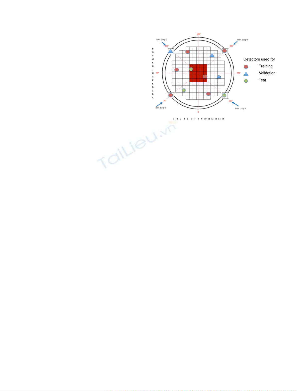
detector, this means specific detector locations have been
split into differing sets to the description in Figure 2 per
axial position of the detectors. Finally, to further test the
robustness of the proposed networks, white Gaussian noise
has been added to the signals at two SNRs, SNR = 5 and 10.
Additionally, for the localisation of fuel assembly
vibrations, the same sub-sampling process has been
undertaken; however, all 56 detectors for a 1 second
sample are considered to be one input into the network.
Therefore, the split of data has been achieved through the
source location of the vibrating fuel assembly, ensuring the
same assembly is not present between sets. The same
process of applying white Gaussian noise have also been
applied to study the effect on the network at SNR = 3 and
SNR = 1, at higher levels of noise, due to the added
robustness of utilising all possible 56 detectors as input.
Fig. 2. Modelled core layout with 8 in-core and 4 ex-core detector
locations shown for one axial plane. Corresponding train, test and
validation detector splits shown, with central 5 5 FA cluster
shown in red.
A. Durrant et al.: EPJ Nuclear Sci. Technol. 5, 20 (2019) 3
4 Approach
ML and more specifically Deep Learning (DL) are a set of
powerful algorithmic approaches for data analytics and
pattern recognition, applying iteratively learnt knowledge
to unseen data for decision making tasks without being
explicitly programmed. DL is a subset of ML, utilising
multiple stacked layers of Artificial Neural Networks
(ANN) inspired by biological neurons to extract
varying levels of information, hence the term deep. The
proposed approaches utilise modern deep learning techni-
ques and architectures extracting valuable pattern infor-
mation from the input signals to iteratively learn the
inverse of the reactor transfer functions.
4.1 3D Convolutional Neural Network
Convolutional Neural Networks (CNNs) [15] are specialised
ANNs designed for spatial feature extraction from data
with known grid-like topologies, i.e. images. CNNs replace
the traditional matrix multiplication of ANNs with the
convolution operation extracting spatial features. More-
over, improving efficiency with the capability of learning
coarse to fine features through the addition of more CNN
layers, extracting complex hierarchical concepts from such
features. Convolutional layers utilise a set of kernels,
learning a corresponding number of filters that to capture
these spatial patterns pertaining to the given input.
Formally, computing the activation of a convolutional
layer ℓand feature-map fat positions i,j,kis given by
aℓ;f½
i;j;k¼fnℓ;f½
i;j;kþbℓ;f½
ð1Þ
where fis a non-linear activation function such as Rectified
Linear Units (ReLU: f(x) = max(0, x)) and bis a learnt bias
nℓ½
i;j;kis given by
nℓ½
i;j;k¼X
X1
x¼0X
Y1
y¼0X
Z1
z¼0
Wℓ½
x;y;z⋅Aℓ1½
iþx;jþy;kþzð2Þ
where W
[ℓ]
is a kernel of learnt weights in layer ℓwith
dimensions XYZ, convolved with the activations from
the previous layer W
[ℓ]*
A
[ℓ1]
. This produces a weighted
sum per location of all points within a kernels receptive field
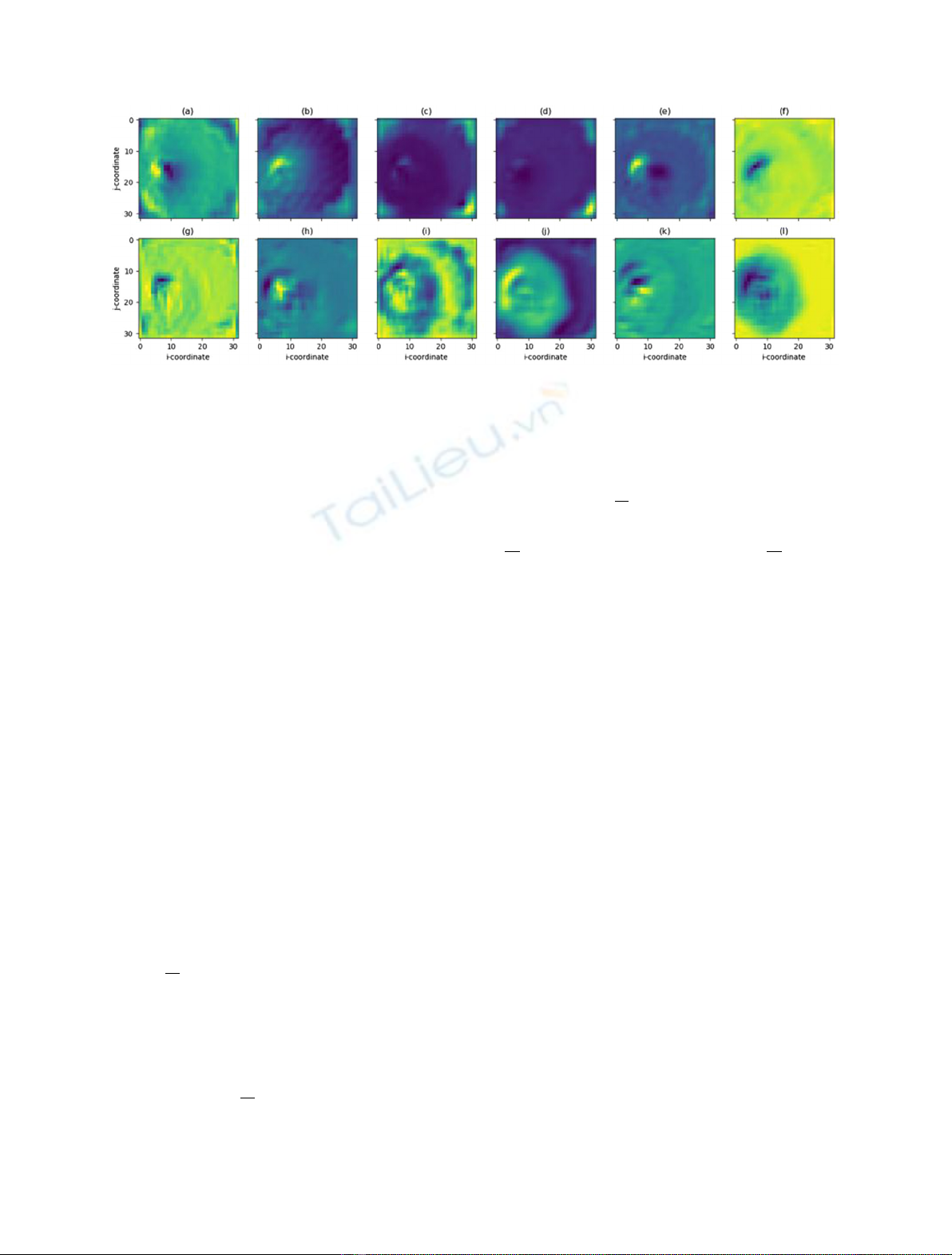
of the previous layers’activations. Visual examples of the
features learnt via the convolution operation can be seen in
Figure 4.
Given the volumetric nature of the signals in the
frequency domain and the task of localisation, it is
necessary to obtain spatial relationships and patterns
within the data volume. Therefore, this work proposes a
modified, densely-connected, 3D-CNN for the volumetric
feature extraction of simulated neutron detector readings
seen depicted in Figure 3.
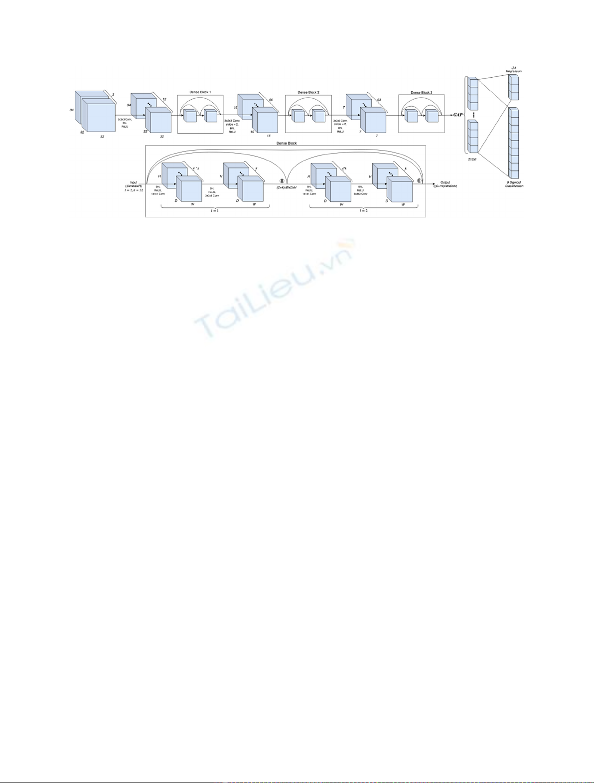
The network depicted in Figure 3 shows the architec-
tural construction of the 3D CNN, comprised of three dense
blocks modified from the 2D variant to allow for the 3D
volumetric input. Dense blocks [16] are an DNN architec-
tural design, utilising several CNN developments, with its
main advantage being the use of dense connections. These
connections allow for a greater flow of information between
layers during the forward and backward pass of the
backpropagation procedure, resulting in the reduction of
vanishing gradients and achieving better performance.
These connections are simply concatenations, where the
ℓth hidden layer H
ℓ
receives as input the feature-maps all
preceding layers within that block
Xℓ¼HℓX0;X1;...;Xℓ1
½ðÞ:ð3Þ
In addition to the dense connections, the network
employs 1 11 kernel convolutions with stride 1 for the
reduction in feature dimensionality following dense con-
nections, furthermore, 1 11 kernels reduce network
parameters whilst increasing network complexity, further
assisting the parameter large 3D convolution operation
[17]. The dense blocks each contain l= 20 layers with
growth rate of k= 6, for further details please refer to [16].
All convolutional layers are followed by the commonplace
procedure: convolutional layer !Batch Normalization
(BN) !and ReLU activation. BN normalises the
activations output by the convolutional layer improving
Fig. 3. The proposed Densely-connected 3D CNN architecture, depicting an example dense block of 2 layers and growth rate of 32.
The Fully-connected and output layers can be seen right of the GAP, each unit represents a classification perturbation type or the
source (i, j, k) location to be regressed.
4 A. Durrant et al.: EPJ Nuclear Sci. Technol. 5, 20 (2019)
network stability, ReLU is a non-linear activation function
with sparse activation, further assisting in the reduction of
vanishing gradients. Furthermore, the proposed network
replaces the pooling operation with strided convolutions
for dimensionality reduction, retaining spatial structural
information from the input vital for the localisation of
perturbation sources.
The last convolutional layer of the network outputs a
representational feature vector of the input of size 256 via
Global Average Pooling (GAP) layer [17], fully connected
to two output layers for perturbation classification and
localisation. GAP directly outputs the spatial average over
the feature maps, resulting in a vector V∈ℝ
m
where mis
the number of feature maps. The output layer for
classification is comprised of 9 non-linear, sigmoid units
each for the occurrence of the individual perturbation types
(nine types as modes of fuel assembly vibration are
considered as classes of perturbation). For localisation
three linear units have been employed each representing
the (i, j, k) coordinates of the perturbation source to be
regressed.
Training the network has been achieved via implement-
ing the multi-task loss approach from [11], minimising the
weighted sum of losses per task (classification and
localisation) with a weight coefficient identifying the
impact each tasks loss in the training procedure. For
classification the network aims to minimise the negative
log-likelihood (NLL)
NLL ¼1
NX
N
i¼1
yi⋅log ^
yi
ðÞþ1þyi
ðÞ⋅log 1 ^
yi
ðÞð4Þ
and for localisation regression, minimises the L2 loss, or
mean squared error (MSE)
MSE ¼1
NX
N
i¼1
jjyi^
yijj2ð5Þ
where y
i
and ^
yiare the true and predicted values of the
network for Nnumber of examples. As previously alluded
the 3D CNN network is trained minimising a weighted sum
of losses
LðX;W;l1;l2Þ¼ 1
NX
N
i¼1
l1
PX
P
p¼1
½yp
1·logðb
yp
1Þþð1yp
1Þ·logð1b
yp
1Þl2
CXjj
C
c¼1
yc
2b
yjjc2
2
"#
i
ð6Þ
where Pand Care the number of perturbation classes and
source location coordinates respectively, l
1
and l
2
are the
manually tuned hyper-parameter weight coefficients for
each task loss, classification and localisation regressing
respectively. This objective is minimised given Xas input
data with respect to Wparameters (weights and biases).
4.2 Long short-term memory, recurrent neural
network
Time domain signals hold temporal information within
their sequential structure, therefore, a differing approach
to previously described is necessary to capture these time-
dependent features. To more appropriately capture the
relationships within the detector signals, Recurrent Neural
Networks (RNN) have been employed. RNNs utilise
recurrence to allow information about previous time-steps
to persist within the network informing current and future
time-step cells across the sequence. RNNs in principle
formulate a non-linear output A
t
from both the input data
x
t
at that given time-step and the activation of the previous
timesteps cell A
t1
, where fis a non-linear activation
function such as hyperbolic tangent (tanh):
At¼fxt;At1
ðÞ:ð7Þ
Long Short-Term Memory (LSTM) [18], a variation of
RNNs have been incorporated in this work for their ability to
learn long term dependencies across long sequences, ideal for
the 100 time-step sequences in question. It achieves this
ability with the use of memory gates, regulating and learning
how much to ‘remember’from previous cell states and how
Fig. 4. Sample of 12 learnt feature-maps from the output of first dense block for the input of vibrating fuel assembly at (8,16) given all
possible detectors. Visually depicting how the differing layers highlight different features of the image. (a) Shows a peak at the source of
vibration, (d) the response on the core barrel, (j) the noise dissipating throughout the core.
A. Durrant et al.: EPJ Nuclear Sci. Technol. 5, 20 (2019) 5




![Bài tập trắc nghiệm Kỹ thuật nhiệt [mới nhất]](https://cdn.tailieu.vn/images/document/thumbnail/2025/20250613/laphong0906/135x160/72191768292573.jpg)
![Bài tập Kỹ thuật nhiệt [Tổng hợp]](https://cdn.tailieu.vn/images/document/thumbnail/2025/20250613/laphong0906/135x160/64951768292574.jpg)

![Bài giảng Năng lượng mới và tái tạo cơ sở [Chuẩn SEO]](https://cdn.tailieu.vn/images/document/thumbnail/2024/20240108/elysale10/135x160/16861767857074.jpg)


