EURASIP Journal on Applied Signal Processing 2005:3, 346–358 c(cid:1) 2005 Hindawi Publishing Corporation
A New Time-Hopping Multiple Access Communication System Simulator: Application to Ultra-Wideband
Galo Nu ˜no-Barrau Departamento de Se˜nales, Sistemas y Radiocomunicaciones, Universidad Polit´ecnica de Madrid, 28040 Madrid, Spain Email: galo@gaps.ssr.upm.es
Jos ´e M. P ´aez-Borrallo Departamento de Se˜nales, Sistemas y Radiocomunicaciones, Universidad Polit´ecnica de Madrid, 28040 Madrid, Spain Email: jmpaez@etsit.upm.es
Received 14 September 2003; Revised 16 May 2004
Time-hopping ultra-wideband technology presents some very attractive features for future indoor wireless systems in terms of achievable transmission rate and multiple access capabilities. This paper develops an algorithm to design time-hopping system simulators specially suitable for ultra-wideband, which takes advantage of some of the specific characteristics of this kind of systems. The algorithm allows an improvement of both the time capabilities and the achievable sampling rate and can be used to research into the influence of different parameters on the performance of the system. An additional result is the validation of a new general performance formula for time-hopping ultra-wideband systems with multipath channels.
Keywords and phrases: ultra-wideband, time hopping, WPAN, spread spectrum, multipath channel, simulation.
1. INTRODUCTION
solving dense multipath interference (a consequence of the extremely high delay resolution of the signals), low con- sumption, high resistance to the interference from other communication systems, low probability of interception, high spatial resolution or the possibility of coexistence with other radio systems in the same frequency bands. After the FCC ruling in February 2003, the development of UWB tech- nology has been accelerated by the entry of new enterprises and research centers that are providing new approaches to solve some of the main problems of UWB systems.
Multiple access (MA) systems based on time-hopping spread-spectrum (TH-SS) techniques have recently started to be taken into consideration as a possible solution for the implementation of the future short-range personal commu- nication systems (PCSs) or wireless personal area networks (WPANs) [1]. So far, the most important TH-SS system has been time-hopping ultra-wideband (TH-UWB), which is characterized by the use of signals with very large relative bandwidths and reduced power spectral densities [2, 3]. Ac- cording to the US Federal Communications Commission’s (FCC) first report and order, an UWB device can be de- fined as any device emitting radio signals with a −10 dB fractional bandwidth greater than 0.2 or a bandwidth of at least 500 MHz at all times of transmission [4]. In TH-UWB, this can be achieved by the pseudorandom transmission of very narrow signals, usually referred to as monocycles or monopulses [5].
This is an open-access article distributed under the Creative Commons Attribution License, which permits unrestricted use, distribution, and reproduction in any medium, provided the original work is properly cited.
TH-UWB presents some characteristics that make these systems very attractive for high-speed WPAN as 802.15.3 or indoor communications [6, 7], such as the possibility of re-
In order to design a real TH-UWB system, many aspects should be taken into careful consideration, such as modu- lation schemes, waveforms design, time-hopping codes, re- ceiver architecture, decision schemes, or channel models, most of them are under discussion at the present moment. Therefore, to develop accurate and flexible simulation tools is necessary to analyze the influence of these factors and to have a deeper perspective of the performance of the system be- fore a physical prototype can be constructed. Unfortunately, the development of a software simulator for UWB has sev- eral difficulties derived from the extremely large sampling rate necessary to process these ultra-wide bandwidth signals. In a straightforward approach with a constant sampling rate, the length of the array that contains the samples of a single bit can be very large, depending on the relationship between the duty cycle and the bit and chip rates. This array should
Link k
Bit 1
Bit 2
Bit 3
Bit 4
Time
A New TH-MA Communication System Simulator: Application to UWB 347
T f
Chip 0 Chip 1 Chip 2 · · · Chip Ns − 2 Chip Ns − 1
Time
pass through different blocks that model the channel and the receiver responses; so a considerable number of operations should be made and consequently the total computing time is very high, even in very fast workstations.
Tc
Slot 0
Slot 1
· · · Slot Nh − 2 Slot Nh − 1
Time
Monocycle transmitted
Some simulators presented in the literature try to avoid this problem by using variable-rate sampling [8]. However, in channels with a considerable number of multipath com- ponents and several users, the necessary computational re- quirements to evaluate and process the possible overlapping between the desired windows and the interfering signals pro- duce high simulation times, specially for low bit error rates (BERs). This fact reduces considerably the efficiency.
Figure 1: Frame structure for TH signals.
In this paper, a new method to design a TH-UWB (or in general TH) communication system simulator is presented. The method takes advantage of some of the properties of this kind of systems in order to provide a very straightforward and fast processing that improves all the previous designs by several orders of magnitude, independently of the sampling rate (which can reach some tens of gigasamples per second) and flexible enough to admit all the different characteristics mentioned above (modulation, channels, sequences, etc.). As an application of the use of the simulator, a new theoreti- cal formula to predict the system performance has been vali- dated, based on the one presented in [2].
Nh slots of length Tc. The monocycle is transmitted in one of these slots (one monocycle per chip), in a position (number of the slot) given by a pseudorandom TH sequence. The data modulation in the monocycles can be in amplitude, phase, or time shift, and the slot length Tc must be large enough to contain the different monocycles.
The bit rate is 1/T f Ns or equivalently 1/TcNhNs. In [9], an M-ary scheme is also proposed, where instead of coding single bits, it is possible to code groups of bits using M-ary monocycle alphabets. In this case, instead of bits, groups of log2(M) bits are transmitted in each symbol (which would be divided into Ns chips with Nh slots each one). This method allows an increment in the bit rate but the receiver complex- ity can make it unsuitable for this kind of systems. This paper is organized as follows. In Section 2, a com- plete mathematical model of a TH system is presented based on the previous research found in the literature. From this model, in Section 3, it is shown how changes can be made in the signal processing to allow the development of an en- hanced linear algorithm to simulate the whole system. Fi- nally, in Section 4, numerical results are provided under dif- ferent sets of parameters to analyze the simulator perfor- mance, including a comparison with other simulators pre- sented in the literature and the validation of the new perfor- mance formula.
Given the kth link, the signal transmitted at the connec- tion point between the modulator and the antenna has the following structure:
(cid:3)
(cid:2)
∞(cid:1)
j Tc −d(k)
j λ−τ(k)
j wtr
0
j=−∞
2. GENERAL MODEL OF A UWB COMMUNICATIONS SYSTEM Aa(k) t − jT f −c(k) s(k)(t) = (1) ,
which is an improved version of the one presented in [2]. The meaning of the terms is explained in the following points.
(i) wtr(t) is the transmitted monocycle. In [10, 11], some possible waveforms for the UWB monocycle have been pro- posed, such as the first, second, and third derivatives of the Gaussian pulse, the Laplacian pulse, the rectangle pulse, or even one period of a sine wave. Moreover, wtr(t) can be base- band, as proposed in [3], high pass or modulated, to comply with FCC regulation.
2.1. Signal description We consider a UWB system composed of Nu different links. These links can correspond to different real users transmit- ting and receiving through different terminals or to different links established between two terminals in order to achieve a higher aggregate bit rate. No further assumptions about the symmetry of these links will be made, so they can be symmet- ric or asymmetric depending on the system functionality (file downloading, video streaming, videoconference, telemetry, etc.). In the case of different terminals, they can be static or mobile and they can be close to one another or relatively far apart, taking into account that so far the main applications of this kind of systems are indoor communications, where distances cannot be too large.
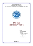
The transmitted signal in one direction of one of the links consists of a series of pulses whose frame structure can be seen in Figure 1. A single bit is composed of Ns chips, each of them with period T f . Each one of the chips is subdivided into In Figure 2, the waveform of a modulated version of the second derivative of the Gaussian pulse is shown. The modu- lation itself is different from “classical” narrowband systems, where the carrier frequency is very high related to the sig- nal bandwidth. In UWB systems, the envelope contains only some periods of the carrier in order to keep a high relative bandwidth.
Link 0
0.8
0
1
1
3
0.6
Time
0.4
τ(k) 0
Link k
0.2
Nh − 1
0
1
2
Time
0
e d u t i l p m A
−0.2
348 EURASIP Journal on Applied Signal Processing
Figure 3: Example of the asynchronism between different links.
−0.4
−0.6
1
2
3
5
6
7
4 Time
8 ×10⁻¹⁰
can make it completely unsuitable in the practice. This could be the reason why most of the work regarding UWB consid- ers just a binary PPM modulation with a delay constant λ as in [2]. In [15], an alternative intrabit coding based on super- orthogonal codes is described that allows the improvement of the bit error probability (BEP) or the increase of the num- ber of links by a factor that is logarithmic with the number of pulses Ns.
Figure 2: Example of the modulated second derivative of the Gaus- sian monocycle. The presence of only 5-carrier periods should be noticed.
j
j } is a sequence of integers with period Np whose values are taken from the range between 0 and Cmax, with Cmax < Nh. The integer c(k) denotes the slot of the jth chip where the monocycle should be transmitted. In [12], an algorithm to easily design these sequences can be found, and in [13, 14], there are complete analyses of the influence of the codes on the power spectral density (PSD) of the signal.
(ii) T f is the frame time or chip period, divided in Nh The slot length Tc must be greater than the monocycle duration plus the maximum delay due to the PPM modula- tion in order to be able to contain all the possible signals of the alphabet. slots of length Tc as it has been previously explained. (iii) The pseudorandom TH code {c(k)
0
(cid:2)
(cid:3)
∞(cid:1)
The aim of the modulation is not only the data trans- mission but also the spectral shaping. An accurate analysis of the influence of data modulation and TH codes, as the one presented in [13], has shown that the combination of PPM and PAM modulations can yield a lower PSD than each of them separately. Therefore, the possibility of combining both schemes should also be taken into careful consideration, not only with the purpose of increasing the data rate but also to lower the PSD, which is crucial in this kind of systems (espe- cially after restrictive FCC ruling). In Figure 4, a conceptual model of the generation of the signal in (1) is presented. Signal Π(t) is defined as
j Tc − d(k)
j λ − τ(k)
0
j=−∞
(iv) The asynchronism between different links is shown by τ(k) as a delay with respect to the beginning of the frame for the first link (from now on, the first link will be consid- ered as the desired signal, and the other links as interference), as represented in Figure 3. t − jT f − c(k) Aa(k) j δ Π(t) = , (2) (v) Pulse-amplitude modulation (PAM). {a(k)
where δ(t) is the Dirac distribution. This signal is introduced in a filter whose impulse response is the shape of the desired monocycle wtr(t), whose output s(k)(t) is transmitted to the channel.
j } is a se- quence of symbols taken from an M-ary alphabet (typically binary) related to the data sequence to be transmitted by the kth link. Depending on the coding scheme, the sequence {a(k) j } can be constant for all the Ns chips or more compli- cated intrabit codes can be applied to provide an additional error protection. The symbols are scaled by the amplitude constant A. The problem of this modulation scheme is that pulse inversion can happen due to the reflections, and that is the reason why it was not considered in [2]. Notwithstand- ing, some manufacturers have proposed a binary antipodal PAM as the modulation scheme for UWB systems.
2.2. Channel model
One of the main problems found in the UWB system simu- lator design is the lack of a well-established channel model for wideband indoor signal propagation. Many propagation measurements and channel models can be found in the lit- erature, but most of them are narrowband in comparison to the extremely wide UWB spectrum, which can go from nearly DC to 11 GHz. Therefore, it is necessary to take ac- curate measurements of the channel prior to developing a complete mathematical channel model. For the last years, a steadily growing number of new analysis and models have appeared based on different sets of measurements, and prob- ably more will appear before one is internationally adopted. (vi) Pulse-position modulation (PPM). Equivalently, the sequence {d(k) j } can be employed as a sequence of time shifts in a PPM modulation. In [9], a complete analysis of a TH- UWB spread-spectrum MA system based on an M-ary PPM modulation is presented, where M different time shifts are applied to the signals. However, even with the advantages de- rived from the use of modulation with M greater than 2, the receiver complexity to handle the severe timing requirements
Link (k)
Data (k)
Asynchronism
A New TH-MA Communication System Simulator: Application to UWB 349
Sequence generator
PPM modulator
c(k) j Tc
λd(k) j
Signal distortion is mainly due to antennas radiation and free-space propagation (where higher frequencies are more attenuated) and it can be represented by an impulse response hdist(t):
τ(k) 0
+
Aa(k) j
×
PAM modulator
Impulse train generator
(6) θ(t) = w(t) ∗ hdist(t),
Π(t)
(cid:2)
L(cid:1)
(cid:3) .
s(k)(t)
where ∗ denotes the convolution product of functions. Therefore, from (5) and (6), a general channel-impulse re- sponse h(k)(t) can be represented (for observation windows, where the channel can be considered as static) as
Waveform generator
l=1
(7) β(k) l δ t − τ(k) l h(k)(t) = hdist(t) ∗
Figure 4: Conceptual model of the UWB signal generation.
As a consequence of that, a TH-UWB simulator should be able to support different channel models with flexibility.
L(cid:1)
In any wireless channel, the received signal is a sum of the replicas (echoes) of the transmitted signal, being related to the reflecting, absorbing, scattering, and/or deflecting ob- jects via which the signal propagates. There is, however, a major difference between UWB and narrowband systems: in a narrowband system, the echoes at the receiver are only at- tenuated, phase-shifted, and delayed, but undistorted, so that the received signal may be modeled as a linear combination of L delayed basic waveforms wtr(t):
(cid:3) .
(cid:2) t − τ(k) l
l=1
The received signal will be then a set of pulses distorted by the channel (independently of their paths) with amplitudes depending both on a random distribution to include the dif- ferent reflection, scattering, and/or diffraction phenomena, and on a deterministic function of the distance and the fre- quency. As it is shown in (7), in general, the channel presents a different response to each link. It could be also reasonable to consider a different channel distortion h(k) dist(t), as it is com- mented in Section 3. Several models have been proposed for the amplitude and delay estimation, as [18] or [19]. One of the commonly agreed points is that the duration of the mul- tipath response for narrow pulses (1-2 nanoseconds or less) in a typical office or residential environment is between 125– 200 nanoseconds depending on the building size and struc- ture. r(k)(t) = (3) β(k) l w
(cid:5)
(cid:4) Nu(cid:1)
The channel also introduces noise and interference to the signal. The noise n(t) can be modeled as additive white Gaus- sian noise (AWGN) with a PSD defined as N0/2 whereas the interference depends on the existence of other electromag- netic signals at the same frequency band. Without taking in- terference into consideration, the received signal in a system with Nu transmitters will be
k=1
L(cid:1)
In UWB systems, the frequency selectivity of the reflec- tion, absorption, scattering, and/or diffraction coefficients of the objects via which the signal propagates can lead to a dis- tortion or reshaping of the transmitted pulses. Furthermore, the distortion and, thus, the shape of the arriving echoes, varies from echo to echo [16]. The received signal is, thus, given as r(t) = s(k)(t) ∗ h(k)(t) + n(t) (8)
(cid:3) ,
(cid:2) t − τ(k) l
l=1
(cid:4)
r(k)(t) = (t)θl (t) (4) β(k) l or equivalently
Nu(cid:1)
L(cid:1)
∞(cid:1)
(cid:2) t − jT f − c(k)
j Tc − d(k) j λ
j β(k) a(k) l θ
j=−∞
k=1
l=1
(cid:5)
(cid:3)
where θl(t) is the received pulse through the lth path. A r(t) =
− τ(k) l
− τ(k) 0
l
+ n(t). (t) and τ(k)
(9)
(cid:2)
(cid:3)
L(cid:1)
j } and {a(k)
2.3. Receiver structure However, in [16], it is also stated that the distortion of the different propagation paths is negligible in a real situation, so (3) could be considered valid, taking into account a slow variation of both β(k) (t). Nevertheless, even if this l model is very straightforward, it is also too simplistic due to not considering any frequency-depending signal distortion, as the one detected in [17]. Therefore, the impulse response should be
l=1
r(k)(t) = (5) β(k) l θ t − τ(k) l
l
l
(t) and τ(k) The UWB receiver must determine the value of sequences {d(k) j } based on the observation at the receiver an- tenna terminals of the received signal r(t) in time intervals whose duration is Ts = NsT f . In order to achieve that, and providing the receiver that can estimate the channel response of the desired link, a RAKE receiver can be implemented (as that is a particular case of (4) with β(k) (t) changing slowly in relation to the observation window.
Hard decision
c(l) j Tc
Link(1)
Ns chips
Sequence generator
0/1
αi
Decoder
Bin decision
τ(l) 0
Synchronization
Template generator
Bit estimation
v(t)
r(t)
Channel
Channel estimation
Bit estimation
α
αi
Correlator
Bin accumulator
Bin accumulator
αi
Soft decision
Decision
350 EURASIP Journal on Applied Signal Processing
Figure 5: Conceptual model of the UWB receiver for the first user.
Figure 6: Hard and soft decision examples. In the hard decision (upper part), the sequence of chips is considered a codeword that is stored in a register prior to its decoding. In the soft decision (lower part), chip statistics are first accumulated in a bit statistic variable α and then the decision is taken.
The signal ϕ(t) changes depending on the type of modu- lation employed. For PAM modulations, it is
ϕ(t) = ˜θ(t) (12)
and it is
ϕ(t) = ˜θ(t) − ˜θ(t − λ) (13)
for binary PPM (this is the one considered in the text, al- though extensions to M symbols can be easily achieved), where ˜θ(t) is the estimated waveform. If both modulations are combined, ϕ(t) depends on the way the information is coded, so different schemes could be employed.
Ns(cid:1)
Once the chip statistics have been calculated, a bit deci- sion should be taken. Two different techniques can be ap- plied: hard and soft decision (see Figure 6). The difference between them is that whereas in the first one, the decisions are taken independently on every chip, in the second one, all the chip statistics are added previously to be decided. In for- mal terms, the bit statistic α for the soft decision is [2]
i=1
α = αi. (14)
the one proposed in [20]) with Lmax < L fingers. This RAKE must be able to capture a large number of different multi- path components (fingers) and combine them to improve the signal-to-noise ratio (SNR). Each one of its Lmax fingers is adapted to a different propagation path, with two possible structures: in a selective RAKE (SRAKE), the Lmax strongest multipath components are chosen, whereas in a partial RAKE (PRAKE), the first arriving ones are selected, yielding a less efficient (but less complex) structure. In order to simplify the receiver structure, it can be considered that the maximum duration of the RAKE fingers τ(1) Lmax is smaller than the chip period T f , so the system is working only on two chips each time. In the vast majority of the described systems, with Tc less than two nanoseconds and low duty cycles, this condi- tion allows the capture of most of the significant multipath components. Nevertheless, all the results shown in the fol- lowing sections can be easily extended to the case τ(1) > T f . Lmax In [21], an adaptive algorithm is presented to derive the optimal template waveform at the receiver that captures the highest amount of energy with the least number of corre- lations. This algorithm takes advantage of the fact that the channel effects are somehow embedded in the received sig- nal, so the optimal template waveform can be computed based on the received signal online. Therefore, it is possible for the receiver to use a template signal adapted to the re- ceived one, providing that this kind of algorithms could be implemented.
In the hard decision, α is the most common value among the decisions of the Ns chips of a bit. This scheme is easier to implement than soft decision, but, in general, less efficient due to the loss of information, as it is commented in [22]. Nevertheless, hard decision can be combined with intrabit coding to provide better performance [15].
(cid:6)
(cid:3)
i Tc
(i+1)T f +τ(1)
0 +c(1)
−c(1)
(cid:2) t −iT f −τ(1)
In order to recover the information, the receiver corre- lates the signal r(t) with the template signal, which should be previously synchronized (see Figure 5). It is necessary for the receiver to know the TH sequence of its transmitter. The statistic for the ith chip is 2.4. Comments on the previous simulators
i Tc
0
i Tc
iT f +τ(1)
0 +c(1)
αi = r(t)×v dt, (10)
(cid:3)
Lmax(cid:1)
where
(cid:2) m ϕ β(1)
m=0
. t − τ(1) m v(t) = (11) So far an analytical model of a whole multiuser UWB com- munication system has been presented. In order to simu- late it, a very straightforward structure could be based on a Monte Carlo simulation method, where a vector of bits is generated and transmitted through a given link. The vector of bits received after decision is compared with the original one and the BEP is estimated as the average number of errors
Multiuser interference
Noise vector
A New TH-MA Communication System Simulator: Application to UWB 351
TH-UWB transmitter
TH-UWB channel
TH-UWB receiver
general, of any TH signal). An additional advantage of this structure is the independence of the simulation time from the sampling rate, which can be as high as necessary without reducing the time capabilities of the system.
0 1 · · · 1 0
0 1 · · · 0 0
X-OR
Vector transmitted
Vector received
0 0 · · · 1 0 Error vector
3. ENHANCED TH SIMULATION ALGORITHM
Figure 7: Simulator schematic as the one described in [8].
The aim of this section is to describe a possible enhanced structure for a TH-UWB simulator. All the results will be provided for the case of soft-decision detection, but it can be easily extended to hard decision just changing from bit simulations to chip simulations and taking into account the possible correlation between noise samples, as it will be ex- plained in the following sections.
3.1. Signal and noise separation: signal processing
i + αn i ,
The first step is the separation between the signal and noise components of every chip statistic. Taking into consideration (9) and (10), a chip statistic αi can be described as between the length of the vector (number of bits transmit- ted). In order to have a good estimation, this length should be at least two orders of magnitude greater than the inverse of the BEP [23]. Thus, hundreds of millions of bits should be processed for a BEP of 10−6. αi = αs (15)
(cid:6)
(cid:2)
i Tc
(i+1)T f +τ(1)
0 +c(1)
− c(1)
where
i Tc
(cid:3) dt,
0
i Tc
iT f +τ(1)
0 +c(1)
t − iT f − τ(1) αs i = rs(t) × v
(cid:5)
(cid:4) Nu(cid:1)
(16)
k=1
(17) rs(t) = s(k)(t) ∗ h(k)(t) ,
(cid:6)
(cid:2)
(cid:3)
i Tc
(i+1)T f +τ(1)
0 +c(1)
−c(1)
is the signal component and This structure is followed by the two simulators described in [8] (see Figure 7). There are two major differences between them, whereas the first one is based on a constant sampling rate and it has the same lengths for the signal and noise vec- tors, in the second one, only the nonzero intervals are sam- pled and noise is only added to those samples that have any influence on the chip statistic. The second approach provides a better performance in the case of low duty-cycle signals, as all the zero samples are ignored. Unfortunately, due to the channel multipath and the multiuser interference (MUI), the received signals present a considerable increment in the duty cycle, so in the end, both approaches present similar perfor- mances in a multiuser/multipath environment.
i Tc
i Tc
iT f +τ(1)
0 +c(1)
αn i = n(t)×v dt (18) t −iT f −τ(1) 0
is the noise contribution to the chip statistic.
(cid:6) t
It would be desirable to extract the effects related to the waveform distortion from those related to the delay in an attempt to simplify the system. It is known that given two functions ψ(t) and ξ(x), with ξ(x) equals to zero out of the interval [0, T],
(cid:7) T − (t − x)
(cid:8) dx|t=τ+T
t−T (cid:6) τ+T
=
The main problem is the length of the vectors. For in- stance, a binary PPM-TH-UWB system with a bit rate of 100 kbps and 1-nanosecond pulses has ten thousands pos- sible chip slots per bit. The necessary sampling rate to avoid aliasing can be higher than 10 gigasamples per second, de- pending on the waveform, so every bit is represented by at least one hundred thousand (100.000) samples. In order to simulate the different system blocks, several operations should be applied on these vectors (convolutions, window- ing, etc.), so the total computing time to estimate a single BEP value for a given set of conditions can be very high, which reduces the simulator utility. ψ(x)ξ ψ(t) ∗ ξ(T − t)|t=τ+T =
τ
ψ(x)ξ(x − τ)dx,
(19)
(cid:5)
(cid:4) Nu(cid:1)
which can be applied to (16):
(cid:8)
|
∗ v
(cid:7) T f − t
i Tc , (20)
(i+1)T f +τ(1)
0 +c(1)
k=1
In order to improve the performance, it would be de- sirable to apply importance sampling methods instead of Monte Carlo. However, to do it efficiently, it is necessary for the noise to have its dimensionality close to one (the number of samples per experiment), and to have low correlation be- tween different experiments. Therefore, the noise should be reduced to a sample per experiment with a low autocorrela- tion. αs i = s(k)(t) ∗ h(k)(t)
In the next section, a simulation structure is presented that achieves a reduction of the noise dimensionality to one and that allows an extremely fast bit processing as a conse- quence of the particular structure of TH-UWB signals (or, in < T f . where v(t) is zero out of the interval [0, T f ] as τ(1) Lmax
352 EURASIP Journal on Applied Signal Processing
ε(k) i, j,l,m
αs
Simulations
Computation of ε(k)
i, j,l,m
Equivalently, applying (9),
(cid:5) (cid:3)
(cid:4) Nu(cid:1)
∞(cid:1)
L(cid:1)
=
(cid:2) t−jT f −c(k)
j Tc−d(k)
j λ−τ(k)
j β(k) a(k) l δ
−τ(k) l
0
Data (fast variation)
(cid:8) |
αs i
j=−∞ l=1 (cid:7) T f − t
k=1 ∗ θ(t) ∗ v
c(1) i Tc
(i+1)T f +τ(1) 0
Channel conditions (slow variation)
.
(21)
Taking into consideration (11), the last term in (23) can be expanded, after some trivial operations, as
Figure 8: Signal processing flowchart. It should be noticed how ε(k) i, j,l,m is only recomputed when the channel conditions change. The main signal simulation loop is in charge of generating data to be calculated (32).
(cid:2)
(cid:3)
Lmax(cid:1)
(cid:8)
∗ δ
(cid:7) T f − t
m δ β(1)
= ϕ(−t) ∗
(cid:7) t + T f
(cid:8) ; (22)
m=0
v t + τ(1) m
This integral will be nonzero only for the values that satisfy
−d(k)
j λ − Tc − η < ε(k)
i, j,l,m < Tc + λ + η − d(k) j λ.
so if we define the transmitted-distorted-received (TDR) waveform Ω(t) as (29)
Ω(t) = θ(−t) ∗ ϕ(t), (23)
(cid:2)
Nu(cid:1)
∞(cid:1)
L(cid:1)
Lmax(cid:1)
then (23) can be rewritten as It can also be expressed with independence of the PPM transmitted data. Thus, for i = 1, . . . , Ns, let { j, k, l, m} ∈ Γ be the set of values that satisfy
j β(k) a(k)
j Tc − d(k) j λ
m δ l β(1)
(cid:9) (cid:9) (cid:9)ε(k)
(cid:9) (cid:9) (cid:9) < Tc + η + λ;
i, j,l,m
j=−∞
m=0
k=1
l=1
(cid:2)
(cid:3)(cid:3)
−
t − jT f − c(k) αs i = (30)
i can be obtained as
− τ(k) 0
(cid:1)
∗ Ω
(cid:8) |
then αs τ(k) l − τ(1) m
(cid:7) T f − t
i Tc
(i+1)T f +τ(1)
0 +c(1)
j β(k) a(k)
(cid:2) m Ω
l β(1)
(cid:3) i, j,l,m + d(k) ε(k) j λ
j,k,l,m∈Γ
. αs i = (31) (24)
Ns(cid:1)
(cid:1)
and the signal component of the bit statistic, in the case of soft decision detection, can be expressed as The TDR signal Ω(t) is very interesting. If we consider no channel distortion and perfect signal estimation, Ω(t) be- comes
j β(k) a(k)
m Ω
l β(1)
(cid:3) (cid:2) i, j,l,m + d(k) ε(k) j λ
i=1
j,k,l,m∈Γ
(25) αs = . ΩPAM(t) = wtr(−t) ∗ wtr(t) (32)
for PAM modulations or
i, j,l,m + d(k)
As ε(k) (26) ΩPPM(t) = wtr(−t) ∗ wtr(t) − wtr(−t) ∗ wtr(t − λ)
for PPM, which are respectively the signal autocorrelation (for PAM) and the subtraction of the autocorrelation and its replica shifted λ (for PPM). In the case of channel distortion, if the channel-impulse response hdist(t) has a duration η, then the TDR will be nonzero in the interval [−Tc − η, Tc + η + λ] (λ = 0 for PAM). Besides, if the distortion hdist(t) is different for every link, then there will be a different TDR Ω(k)(t) for each link.
(cid:3)
(cid:2)
(cid:3) Tc+
(cid:2) (cid:3) +
−τ(1) 0
i, j,l,m is independent of the data, it can be computed only one time for a whole sequence of transmitted bits (see Figure 8), and so the simulation operations to evaluate (32) will be reduced, which results in a considerable time saving. Another big difference with the “traditional” simulators is the waveform processing, based on the access at a partic- ular TDR position given by ε(k) j λ, making it unnec- essary to operate with the signal samples every simulation. Consequently, the sampling rate can be raised with the only penalty of increasing the TDR length, which could make the access slower. Notwithstanding, this effect is negligible as it will be tested in the next section. Therefore, it can be consid- ered that the simulation speed is approximately independent of the sampling rate.
If we apply now the reciprocal change of (19) and define (cid:2) c(k) j −c(1) i , (27) τ(k) l −τ(1) m τ(k) 0 ε(k) i, j,l,m =( j−i)T f +
(cid:2)
(cid:2)
i as (cid:6) T f
(cid:1)
Ns(cid:1)
Nu(cid:1)
(cid:1)
In the case of links with different TDR, (32) results in then we can express αs
(cid:3) .
j β(k) a(k)
j β(k) a(k)
m Ω(k)
l β(1) m
l β(1)
(cid:3) i, j,l,m − d(k) Ω(t)dt. (28) j λ
i, j,l,m + d(k) ε(k) j λ
0
i=1
j,k,l,m
k=1
j,l,m∈Γ(k)
δ t − ε(k) αs = αs i = (33)
A New TH-MA Communication System Simulator: Application to UWB 353
Lmax
Ns
i
Nu
τ(1)
tk j
r
3.2. Noise processing
T
T f
+
+
|ζ (k)
Is r − τ(1)m| < Tc + η?
ζ−1 ζ0
P
pkl
Nu
Yes
No
L
Store ε(k)
k, j, l, m
Store β(k)
i+r, j,l,m in E l β(1) m
(cid:10)
(cid:2)
Ns(cid:1)
(cid:3)(cid:9) (cid:9) (cid:9)
Importance sampling, as it is described in [23], allows a con- siderable decrease of the simulation time by reducing the number of experiments necessary to calculate a single BEP value. In order to apply importance sampling under opti- mum conditions, the experiments should be independent and the noise dimensionality should be close to one. If we apply (19) to (18), the noise component αn can be expressed as
− c(1)
i − Tc
(cid:11) ;
0
T f
αn = T f − t − iT f − τ(1) n(t) ∗ v
Figure 9: Matrix E calculation flowchart.
i=1
(34)
First of all we should define the matrices T (chip posi- tion) and P (channel delay) as
,
· · · .. . · · ·
c(1) Ns c(1) 1 T =
0
L
c(Nu) 1 Tc + T f + τ(1) 0 ... Tc + T f + τ(Nu) 0 so αn is the sum of Ns samples of a filtered Gaussian stochas- tic process. As the interference between adjacent bits is al- most negligible (it is reduced to the possible interference be- tween the last chip RAKE and the first chip one), and αn can be modeled as a Gaussian white process with variance σ 2 n, in the case of hard decision detection, αn i is also a Gaussian se- quence, but its autocorrelation should be computed accord- ing to the chip interference.
. P =
L
To apply the importance sampling, it is just necessary to emphasize αn standard deviation σn by a factor γ (whose op- timum value is around 4) [23]: Tc + NsT f + τ(1) 0 ... Tc + NsT f + τ(Nu) c(Nu) Ns · · · τ(1) ... .. . · · · τ(Nu) τ(1) 1 ... τ(Nu) 1 (38) σ (cid:4)2 n. n = γ2σ 2 (35)
In order to compute ε(k) The new noise component αn(cid:4)
should be added to the sig- nal one αs and the BEP of a soft decision binary system can be computed as
(cid:12)Ne e=1 Ne
i, j,l,m, we choose an element tk j of T and another pkl of P (see Figure 9), 1, . . . , k, . . . , Nu, 1, . . . , j, . . . , Ns, 1, . . . , l, . . . , L, and we add them. The result is the position of the lth received echo of jth chip of the kth link. We can calculate i (position in the first link frame) as (cid:5)(tk j + pkl)/T f (cid:6), where (cid:5)·(cid:6) denotes “the maximum integer smaller than this value.” This chip affects both the ith and the (i − 1)th receiver windows (due to the RAKE length). Thus, the two possible relative positions will be
ψe (36) BEP = ,
(cid:8)
(cid:7) tk j + pkl
− c(k) (i+r)
e )2/2σ 2 n ,
r −τ(1)
where Ne is the number of experiments (number of trans- mitted bits) and ζ (k) r = Tc − (i + r)T f , r = −1, 0. (39) ψe = 0 we if no error occurred in the jth experiment, if an error occurred in the jth experiment, These positions affect we = γe(1−1/γ2)(αn(cid:4) (37)
i+r, j,l,m
is the emphasized noise component of the eth bit where αn(cid:4) e (experiment).
=
the decision if (30) is veri- fied; therefore we can compute all the values that satisfy |ε(k) i+r, j,l,m| = |ζ (k) m | < Tc +η, 1, . . . , m, . . . , Lmax, r = −1, 0, and we store them in the row vectors e(k), with a length infe- rior to 2LmaxLNs. The elements of e(k) are the values ε(k) that verify (30). Finally, we define the matrix E as
.
E = (40) Whereas in the soft decision detection, the experiments are related to transmitted bits, in the hard decision, they cope with chip transmission. Once the chip error rate (CEP) is known, the BEP can be found applying the gain due to the intrachip code. e1Q e11 · · · ... ... . .. eNu1 · · · eNuQ e(1) e(2) ... e(Nu) 3.3. Example: PAM-TH-UWB simulator
As an example of the algorithm, we show a brief description of a PAM-TH-UWB simulator with soft decision detection. It will be a particularization of the general algorithm for the case of absence of PPM (the design of PPM or hybrid simu- lators is equivalent). Matrix E should be recalculated only when the chan- nel conditions change. Depending on the channel coherence time and the bit rate, it is possible to find the number of bits K that can be simulated without altering E. The size of E will be Nu × Q, where Q (number of components of the largest
White Gaussian noise αn
Amplitudes β(k) l β(1) m
A
354 EURASIP Journal on Applied Signal Processing
size of Ω(t), so it has little impact on the total computing time. A is in charge of controlling the SNR, thus, given a waveform Ω(t), A can be defined as
E
√
µ(k)
e(k)
×
×
Accumulator
+
(cid:3)2
α
Ω
(cid:12)Lmax m=1
α(k)
Decision
· · ·
0 1
1 0
Link (1)
Nu
A = SNR (cid:2) σn, (44) β(1) m Ω(0)
0
0 1 · · · 0 0
0 1 · · · 0 1
where σn is the noise standard deviation, which can be set to one. Therefore, the decision variable α is defined as
X-OR
K
K Vector transmitted
Vector recieved
0 0 · · · 0 1
(45) α = αs + X,
K Error vector
where X is a zero-mean Gaussian random variable with vari- ance γ2 (emphasis factor).
4. ALGORITHM PERFORMANCE
Figure 10: Error vector calculation flowchart.
4.1. Time performance
Speaking about time performance, three facts should be re- marked:
l β(1)
e(k)) depends on the channel and RAKE structure, its average value is in general inferior to 2LmaxLNs/Nu, and in the case of no overlapping of the RAKE windows, this value is smaller than 2LNs/Nu. The rows whose length is less than Q are com- pleted with zeros. (1) computational time grows linearly with the number of users, the number of chips, the channel length, and the number of fingers; (2) computational time is independent of the sampling frequency;
(3) the total simulation time per bit is steadily reduced as the SNR (and consequently the number of simulations per bit) increases. Not only are the valid ε(k) i+r, j,l,m values stored, but also their corresponding amplitudes β(k) m . It should be noticed how the algorithm complexity is linear with Nu (number of users), Ns (number of chips per bit), L (number of multipath components), and Lmax (number of fingers), as it will be an- alyzed in the following section.
The first statement can be seen in Figure 11, with the rep- resentation of the computational time per bit in relation to the number of chips and to the number of multipath com- ponents. A linear behavior that is equivalent to the number of users and the number of fingers can be seen, which is due to the simulator structure.
The second part of the algorithm develops the im- portance sampling simulation method, as represented in Figure 10. There it can be seen how the values stored in E, which represent time positions in the TDR waveform, are used to generate their correspondent values, which should be multiplied by their amplitudes and the transmitted data. Therefore, the vector J can be defined as
J = A (41)
a(1)µ(1) a(2)µ(2) ... a(Nu)µ(Nu)
(cid:2)
Q(cid:1)
(cid:1)
(cid:8)
with
=
(cid:7) ekq
m Ω
(cid:3) . (42)
q=1
i, j,k,l,m∈Γ
µ(k) = Ω β(k) l β(1) β(1) mq β(k) lq ε(k) i, j,l,m
Nu(cid:1)
Matrix J stores the information about the desired signal Aa(1)µ(1) and the MUI:
k=2
MUI = A a(k)µ(k); (43)
The effect of the sampling frequency on time perfor- mance can be seen in Figure 12. There it is shown how there is no dependence between the bit simulation time and the sampling frequency. Therefore, a very high accuracy can be obtained without affecting the simulation time, which is a very important feature of the algorithm, and which can be easily extended to other communication system simulators. In Table 1, a comparison of simulation times per bit as the SNR grows under a fixed set of conditions (Tc = 1 nanosecond, Nh = 32 slots, Nu = 1 link, λ = 180 picosec- onds, L = 500 paths, Ns = 1, and Lmax = 1 finger) is pre- sented. A steady reduction in the computational time per bit for the enhanced simulator can be seen. As it was commented in the previous section, the evaluation of E consumes a fixed time independently of the number of simulations. The higher the SNR is, the lower the BEP is, and so a larger number of simulations are required. Therefore, the fixed time is dis- tributed among a bigger number of bits and, consequently, its influence on the bit time is smaller. All the simulations have been done in Matlab with a Pen- therefore the component αs is the sum of both. It is impor- tant to notice how the sampling rate fs only determines the tium IV 1600 MHz with 128 MHz RAM.
0.4
4
e m
i t
3
0.39
2
t i b r e p
0.38
1
l a n o i t a t u p m o C
t i b r e p e m
0
i t
0.37
0
5
10
15
20
25
30
35
Number of chips
0.36
0.4
0.35
e m
l a n o i t a t u p m o C
i t
0.3
0.34
0.2
t i b r e p
0.33
0.1
50
100
150
200
250
300
l a n o i t a t u p m o C
Number of samples per chip
0 10
20
30
40
50
60
70
80
Number of multipath components
A New TH-MA Communication System Simulator: Application to UWB 355
Figure 12: Effect of the sampling rate on the computational time (per bit) for a PPM-TH-UWB system with Tc = 1 nanosecond, Nh = 1024 slots, Nu = 50 links, λ = 180 picoseconds, L = 100 paths, Ns = 4, and Lmax = 10 fingers.
Figure 11: Computational time (per bit) for a PPM-TH-UWB sys- tem with Tc = 1 nanosecond, Nh = 1024 slots, Nu = 50 links, fs = 200 GHz, λ = 180 picoseconds, and Lmax = 10 fingers. In the upper one, L is set to 100 paths and in the lower one, Ns is 4 chips/bit.
Table 1: Simulation times per bit for the simulation chain described in this paper.
SNR 4 5 6 7 8
Enhanced 0.0039 s 0.0016 s 0.0009 s 0.0005 s 0.0003 s
Table 2: Comparison of simulation times per bit for the simulation chains presented in [8].
In Table 2, the simulation times per bit of the two simu- lators presented in [8] are shown under equivalent parame- ters (Nh, L, etc.). The platforms where the simulations were done are unknown, so there is no possible comparison with Table 1. However, it should be noticed that the times pre- sented in [8] are constant with the SNR, so the total time will grow exponentially with the SNR. It is also important to remark that only two years separate between [8] and this pa- per, but the time performance has been improved by more than two orders of magnitude.
4.2. Comparison with theoretical results
SNR 4 5 6 7 8
Variable rate 0.0863 s 0.0863 s 0.0860 s 0.0862 s 0.0863 s
Fixed rate 0.2434 s 0.2428 s 0.2427 s 0.2425 s 0.2354 s
(cid:6) ∞
where
x
e−y2/2d y. (48) Q(x) = 1√ 2π
(cid:8)
Equation (47) can be equivalently expressed as
(cid:7) Nu (cid:28)
(cid:29)
(cid:31)−1
(cid:6) ∞
(cid:30)2
Nu(cid:1)
=
(cid:27)2ds
(cid:22)(cid:23)
(cid:26) Ω(s)
(cid:8)(cid:24)
−∞
k=2
(cid:7) Nu
(cid:8)
(cid:7) Nu
(cid:8)2
=
SNR In (47), a theoretical analysis of the performance of a PPM- TH-UWB systems under certain restrictions is presented, based on the one presented in [2] by Win and Scholtz. In or- der to validate the algorithm, we have decided to test the nu- merical results against the theoretical response. This analysis does not take into consideration explicitly neither the multi- path characteristics of the channel nor the RAKE structure— only the signal distortion (where the multipath could be em- bedded). Under the assumptions of independent links and random sequence selections (with Cmax < Nh/2), the MUI can be modeled as Gaussian and the BEP for soft decision can be expressed as + , A(k) A(1) 1 SNR(1) 1 NsT f Ω(0)2 BEP = Q SNR , (46) (49) SNR
(cid:26) (cid:25) ∞
(cid:7) A(1)Ns (cid:8)2(cid:7)
(cid:7) A(k)
(cid:25) ∞ −∞ θ(t)ϕ(t)dt (cid:8) (cid:25) ∞ −∞
−∞ θ(t − s)ϕ(t)dt
(cid:12)Nu k=2
(cid:27)2ds (47)
, Ns/T f σ 2n + where SNR(1) is the signal-to-noise ratio in the single-user case (without MUI). In Figure 13, it can be seen how the as- sumption of a Gaussian distribution of the MUI is valid un- der the assumption of no multipath response. It yields the
9000
100
8000
10−1
7000
6000
10−2
5000
P E B
4000
10−3
3000
s e c n e r r u c c o f o r e b m u N
2000
10−4
1000
10−5
0 −10 −8 −6 −4 −2
0
2
4
6
8
−4
−2
0
2
6
8
10
12
Amplitude
10 ×10−2
4 SNR
Simulated Theoretical
356 EURASIP Journal on Applied Signal Processing
Figure 13: Histogram of the distribution of the MUI for a PPM- TH-UWB system with Tc = 1 nanosecond, Nh = 1024 slots, Nu = 900 links, λ = 180 picoseconds, Ns = 64, and no multipath. The number of simulations is 330.503. The Gaussian distribution of the interference can be noticed. The theoretical Gaussian envelope can be seen, with a mean value of 0.006 and a standard deviation of 0.0225.
Figure 14: Comparison between the simulated response and the theoretical response (47) for a PPM-TH-UWB system with Tc = 1 nanosecond, Nh = 1024 slots, Nu = 900 links, λ = 180 picoseconds, Ns = 64, and no multipath. The number of simulations per point for SNR = 10 and 12 was one order of magnitude higher than the expected BEP.
L(cid:1)
(cid:3)2
performance shown in Figure 14. It is important to remark that for BEP lower than the inverse of the number of sim- ulations, divergences between the theoretical and simulated responses may appear in the high SNR region of the graphic (right-hand side). where χ2 channel(k) is the mean square value of the amplitude coefficients of the kth channel-impulse response, and ¯βRAKE and χ2 RAKE are, respectively, the mean and the mean square values of the RAKE coefficients of the first link receiver. If no statistical channel description is available, these values can be easily estimated as
(cid:2) β(k) l
χ2 channel(k)
= 1 L
l=1
Lmax(cid:1)
,
¯β RAKE
= 1 Lmax
m=1 (cid:2)
Lmax(cid:1)
(51) β(1) m , These divergences are due to the fact that the importance sampling only optimizes the number of simulations in the left region, where the noise interference is the main cause of errors. Thus, when the MUI is larger than the noise interfer- ence, it is necessary to increase the number of simulations to the equivalent of a situation without importance sampling to avoid such divergences.
(cid:3)2
χ2 RAKE
= 1 Lmax
m=1
4.3. Theoretical performance in a multipath . β(1) m environment
l
The empirical validation of (50) is shown in Figure 15. There it can be seen how (50) describes accurately the system performance.
m ϕ(t − τ(1) β(1)
(cid:8)
There are several approaches where the simulator can be very useful, including the possibility of optimization by sim- ulation, where given a set of constraints, a parameter is op- timized by simulating its performance and finding the op- timum value. This can be achieved thanks to the algorithm speed.
(cid:31)−1
(cid:6) ∞
(cid:27)2ds
=
(cid:26) Ω(s)
5. CONCLUSIONS SNR The theoretical model previously commented works prop- erly in the absence of multipath propagation, but does not explicitly include the multipath channel response or the RAKE structure. Thus, the simulator presented can be em- ployed, for example, to validate an extension of this model, as the one presented by us in (50). The development is sim- ple. On one hand, the L paths of each link can be modeled as (Nu − 1)L independent sources, with amplitudes β(k) . On the other hand, the template waveform changes from ϕ(t) to (cid:12)Lmax m ). If we calculate the average values for the m=1 MUI, we get (cid:7) Nu (cid:28)
−∞
(cid:12)Nu ¯β2 L k=2 RAKE NsT f Lmaxχ2
RAKE
, + 1 SNR(1) χ2 channel(k) Ω(0)2 Under a linear description of a TH system with a multipath channel, it is possible to reduce the simulation process to a se- ries of arithmetical operations, avoiding any filtering or con- volutions, which are operations that consume a great amount (50)
100
A New TH-MA Communication System Simulator: Application to UWB 357
network for multimedia PCS,” in Proc. IEEE 4th Annual Net- world+Interop Conference, pp. 101–108, Las Vegas, Nev, USA, May 1997.
10−1
spread-spectrum impulse
[2] M. Z. Win and R. A. Scholtz, “Ultra-wide bandwidth time- radio for wireless IEEE Trans. Commun.,
hopping multiple-access communications,” vol. 48, no. 4, pp. 679–689, 2000.
10−2
P E B
10−3
10−4
[3] M. Z. Win and R. A. Scholtz, “Impulse radio: how it works,” IEEE Communications Letters, vol. 2, no. 2, pp. 36–38, 1998. [4] Federal Communications Commission (FCC), “Revision of Part 15 of the commission’s rules regarding ultra wideband transmission systems,” First Report and Order, ET Docket 98–153, April 2002, FCC 02-48, Adapted: February Released: April 2002. [5] J. T. Conroy,
10−5
−4
−2
0
2
6
8
10
12
4 SNR
“Spectral characteristics of monopulse com- munication signals,” M.S. thesis, Department of Electrical and Computer Engineering, Illinois Institute of Technology, Chicago, Ill, USA, 1997.
[6] C. Razzell, D. Birru, B. Redman-White, and S. Kerry (Philips), “An alternate high-rate PHY for wireless personal area net- works,” IEEE 802.15-03/125r2, March 2003.
New expression Simulated Theoretical
[7] G. Shor (Wisair), “UWB multiband alternate physical layer
for TG 802.15.3a,” IEEE 802.15-03/151r3, May 2003.
[8] Whyless Project, “Air interface concept (including channel model),” IST-2000-25197, Deliverable D5.1, January 2002. [9] F. Ramirez-Mireles, “Performance of ultrawideband SSMA using time hopping and M-ary PPM,” IEEE J. Select. Areas Commun., vol. 19, no. 6, pp. 1186–1196, 2001.
Figure 15: Comparison between the simulated response and the two theoretical expressions (the one denoted as “theoretical” is based on Scholtz’s formula (47), and “new expression” is the for- mula presented in this paper in (50)) for a PPM-TH-UWB system with Tc = 1 nanosecond, Nh = 1024 slots, Nu = 300 links, λ = 180 picoseconds, Ns = 16, L = 80, and Lmax = 10 fingers. It can be seen how (50) describes exactly the behavior of the simulated response.
[10] J. T. Conroy, J. L. LoCicero, and D. R. Ucci, “Communica- tion techniques using monopulse waveforms,” in Proc. IEEE Military Communications Conference Proceedings (MILCOM ’99), vol. 2, pp. 1181–1185, Atlantic City, NJ, USA, October– November 1999.
of computational time. Following this philosophy, in this pa- per, an algorithm to design TH-UWB simulators has been outlined and its performance has been tested.
[12] M. S. Iacobucci and M.-G. Di Benedetto,
[11] X. Chen and S. Kiaei, “Monocycle shapes for ultra-wideband system,” in Proc. IEEE Int. Symp. Circuits and Systems (ISCAS ’02), vol. 1, pp. 1579–1600, Scottsdale, Ariz, USA, May 2002. “Time hopping codes in impulse radio multiple access communication sys- tems,” in Proc. International Workshop on 3G Infrastructure and Services, pp. 171–175, Athens, Greece, July 2001.
[13] J. Romme and L. Piazzo, “On the power spectral density of time-hopping impulse radio,” in Proc. IEEE Conference on Ultra Wideband Systems and Technologies (UWBST ’02), pp. 241–244, Baltimore, Md, USA, May 2002.
[14] M. Z. Win, “On the power spectral density of digital pulse streams generated by M-ary cyclostationary sequences in the presence of stationary timing jitter,” IEEE Trans. Commun., vol. 46, no. 9, pp. 1135–1145, 1998.
As an example of the simulator utility, an improved the- oretical equation of the performance of TH-UWB systems in the presence of multipath distortion has been proposed and validated thanks to the simulated response. Besides, there are several possible applications of the simulator, from code test- ing to optimization by simulation, which can be explored in the future. It is also interesting to notice the possibility, men- tioned in the text, of combining PAM and PPM modulations to achieve not a higher data rate, but a greater randomness that yields a lower spectral density by reducing its peaks. As spectral control is a critical issue in the development of UWB systems, this can be an interesting approach, instead of a re- duction of the transmitted power.
ACKNOWLEDGMENTS
[15] A. R. Forouzan, M. Nasiri-Kenari, and J. A. Salehi, “Perfor- mance analysis of ultrawideband time-hopping code division multiple access systems: uncoded and coded scheme,” in Proc. IEEE International Conference on Communications (ICC ’01), vol. 10, pp. 3017–3021, Helsinki, Finland, June 2001.
[16] D. Cassioli, M. Z. Win, and A. F. Molisch, “The ultra-wide bandwidth indoor channel: from statistical model to simula- tions,” IEEE J. Select. Areas Commun., vol. 20, no. 6, pp. 1247– 1257, 2002.
The authors would like to thank Mr. Iker Almandoz and Mr. Jon Berakoechea for their reviews and comments on the text. They also thank Mr. Javier Jim´enez Leube from the Univer- sidad Polit´ecnica de Madrid and Mr. Fernando Mojica from ´Ecole Polytechnique de Montr´eal for their support and en- couragement.
[17] J. Kunisch and J. Pamp, “Measurement results and model- ing aspects for the UWB radio channel,” in Proc. IEEE Con- ference on Ultra Wideband Systems and Technologies (UWBST ’02), pp. 19–24, Baltimore, Md, USA, May 2002.
REFERENCES
[18] A. Alvarez, G. Valera, M. Lobeira, R. P. Torres, and J. L. Garc´ıa, “UWB channel model contribution from ACORDE and Uni- versity of Cantabria,” in 21st Meeting of the IEEE 802.15 SG3a, Koloa, Hawaii, USA, November 2002.
[1] M. Z. Win, J. Ju, X. Qiu, V. O. K. Li, and R. A. Scholtz, “ATM based ultra-wide bandwidth multiple-access radio
358 EURASIP Journal on Applied Signal Processing