Hindawi Publishing Corporation EURASIP Journal on Advances in Signal Processing Volume 2007, Article ID 87046, 22 pages doi:10.1155/2007/87046
Research Article Design and Implementation of Numerical Linear Algebra Algorithms on Fixed Point DSPs
1 DSP Emerging End Equipment, Texas Instruments Inc., 12203 SW Freeway, MS722, Stafford, TX 77477, USA 2 Coordinated Science Laboratory, Department of Electrical and Computer Engineering, University of Illinois at Urbana-Champaign, 1308 West Main Street, Urbana, IL 61801, USA 3 Application Specific Products, Texas Instruments Inc., 12203 SW Freeway, MS701, Stafford, TX 77477, USA
Zoran Nikoli´c,1 Ha Thai Nguyen,2 and Gene Frantz3
Received 29 September 2006; Revised 19 January 2007; Accepted 11 April 2007
Recommended by Nicola Mastronardi
Numerical linear algebra algorithms use the inherent elegance of matrix formulations and are usually implemented using C/C++ floating point representation. The system implementation is faced with practical constraints because these algorithms usually need to run in real time on fixed point digital signal processors (DSPs) to reduce total hardware costs. Converting the simulation model to fixed point arithmetic and then porting it to a target DSP device is a difficult and time-consuming process. In this paper, we analyze the conversion process. We transformed selected linear algebra algorithms from floating point to fixed point arithmetic, and compared real-time requirements and performance between the fixed point DSP and floating point DSP algorithm implementations. We also introduce an advanced code optimization and an implementation by DSP-specific, fixed point C code generation. By using the techniques described in the paper, speed can be increased by a factor of up to 10 compared to floating point emulation on fixed point hardware.
Copyright © 2007 Zoran Nikoli´c et al. This is an open access article distributed under the Creative Commons Attribution License, which permits unrestricted use, distribution, and reproduction in any medium, provided the original work is properly cited.
1. INTRODUCTION
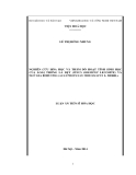
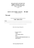
ing point processors offer high precision and wide dynamic range. Fixed point DSP devices are preferred over floating point devices in systems that are constrained by chip size, throughput, price-per-device, and power consumption [5]. Fixed point realizations vastly outperform floating point re- alizations with regard to these criteria. Figure 1 shows a chart on how DSP performance has increased over the last decade. The performance in this chart is characterized by number of multiply and accumulate (MAC) operations that can execute in parallel. The latest fixed point DSP processors run at clock rates that are approximately three times higher and perform four times more 16 × 16 MAC operations in parallel than floating point DSPs.
Numerical analysis motivated the development of the earli- est computers. During the last few decades linear algebra has played an important role in advances being made in the area of digital signal processing, systems, and control [1]. Numer- ical algebra tools—such as eigenvalue and singular value de- composition, least squares, updating and downdating—are an essential part of signal processing [2], data fitting, Kalman filters [3], and vision and motion analysis. Computational and implementational aspects of numerical linear algebraic algorithms have strongly influenced the ways in which com- munications, computer vision, and signal processing prob- lems are being solved. These algorithms depend on high data throughput and high speed computations for real-time per- formance.
Therefore, there is considerable interest in making float- ing point implementations of numerical linear algebra algo- rithms amenable to fixed point implementation. In this pa- per, we investigate whether the fixed point DSPs are capable of handling linear numerical algebra algorithms efficiently and accurately enough to be effective in real time, and we look at how they compare to floating point DSPs.
Today’s fixed point processors are entering a performance realm where they can satisfy some floating point needs with- out requiring a floating point processor. Choosing among DSPs are divided into two broad categories: fixed point and floating point [4]. Numerical algebra algorithms often rely on floating point arithmetic and long word lengths for high precision, whereas digital hardware implementations of these algorithms need fixed point representation to reduce total hardware costs. In general, the cutting-edge, fixed point families tend to be fast, low power and low cost, while float-
105
Floating point DSP
TMS320C64x+
e g n a r
104
TMS320C64x
Overlap zone
c i m a n y D
S / ) s n o i t a r e p o e t a l u m u c c a d n a
TMS320C62x
103
Fixed point DSP
y l p i t l u m
TMS320C6713 TMS320C67x+
TMS320C6711
TMS320C6701
DSP cost and power consumption
f o s n o i l l i
M
102
(
(a)
1996 1997 1998 1999 2000 2001 2002 2003 2004 2005 2006 2007 Year
Fixed point DSP Floating point DSP
Fixed point algorithm implementation on fixed point DSP
2 EURASIP Journal on Advances in Signal Processing
Figure 1: DSP performance trend.
Fixed point algorithm implementation on floating point DSP
Floating point algorithm implementation on fixed point DSP
Floating point algorithm implementation on floating point DSP
Software development cost
(b)
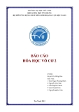
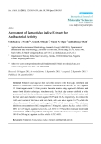
floating point and extended-precision fixed point allows de- signers to balance dynamic range and precision on an as- needed basis, thus giving them a new level of control over DSP system implementations. The overlap between fixed point and floating point DSPs is shown in Figure 2(a).
Figure 2: Fixed point and floating point DSP pros and cons.
Floating point algorithm implementation
r o C P
n o i t a t s k r o w
t n e m n o r i v n e
t n e m p o l e v e d
Ok?
Mapping of a floating point algorithm to a floating point DSP target
t e g r a t / P S D
t n e m n o r i v n e
t n e m p o l e v e d
The modeling efficiency level on the floating point is high and the floating point models offer a maximum degree of reusability. Converting the simulation model to fixed point arithmetic and then porting it to a target device is a time con- suming and difficult process. DSP devices have very different instruction sets, so an implementation on one device cannot be ported easily to another device if it fails to achieve suffi- cient quality. Therefore, development cost tends to be lower for floating point systems (Figure 2(b)).
DSP-specific optimizations
Designers with applications that require only minimal amounts of floating point functionality are caught in an “overlap zone,” and they are often forced to move to higher- cost floating point devices. Today however, fixed point pro- cessors are running at high enough clock speeds for designer to combine floating point emulation and fixed point arith- metic in order to meet real-time deadlines. This allows a tradeoff between computational efficiency of floating point and low cost and low power of fixed point. In this paper, we are trying to extend the “overlap zone” and we investigate fixed point implementation of a truly float-intensive applica- tion, such as numerical linear algebra.
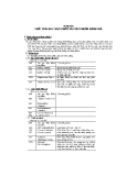
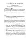
A typical design flow of a floating point system targeted for implementation on a floating point DSP is shown in Figure 3.
Figure 3: Floating point design process.
The design flow begins with algorithm implementation in floating point on a PC or workstation. The floating point system description is analyzed by means of simulation with- out taking the quantization effects into account. The mod- eling efficiency on the floating point level is high and the floating point models offer a maximum degree of reusabil- ity [6, 7]. C/C++ is still the most popular method for de- scribing numerical linear algebra algorithms. The algorithm development in floating point C/C++ can be easily mapped to a floating point target DSP during implementation.
Floating point algorithm implementation
Ok?
System partitioning
The partitioning is based on performance
r o C P
Range estimation
Only critical sections are selected for conversion to fixed point
n o i t a t s k r o w
t n e m n o r i v n e
t n e m p o l e v e d
Bit-true fixed point simulation (e.g., in systemC)
Quantization/ bit-true fixed point algorithm implementation
OK?
Mapping of the fixed point algorithm to a fixed point DSP target
t e g r a t / P S D
t n e m n o r i v n e
t n e m p o l e v e d
DSP-specific optimizations
Zoran Nikoli´c et al. 3
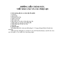
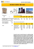
Figure 4: Fixed point design process.
point arithmetic. The system is divided into subsections and each subsection is benchmarked for performance. Based on the benchmark results functions critical to system per- formance are identified. To improve overall system perfor- mance, only the critical floating point functions can be con- verted to fixed point representation.
There are several program languages and block diagram- based CAD tools that support fixed point data types [6, 8], but C language is still more flexible for the development of digital signal processing programs containing machine vision and control intensive algorithms. Therefore, design flow— in a case when the floating point implementation needs to be mapped to fixed point—is more complicated for two rea- sons:
(i) it is difficult to find fixed point system representa- tion that optimally maps to system model developed in floating point;
In a next step towards fixed point system implementa- tion, a fixed exponent is assigned to every operand. Deter- mining the optimum fixed point representation can be time- consuming if assignments are performed by trial and error. Often more than 50% of the implementation time is spent on the algorithmic transformation to the fixed point level for complex designs once the floating point model has been specified [9]. The major reasons for this bottleneck are the following: (ii) C/C++ does not support fixed point formats. Model- ing of a bit-true fixed point system in C/C++ is diffi- cult and slow.
(i) the quantization is generally highly dependent on the stimuli applied;
(ii) analytical methods for evaluating the fixed point per- formance based on signal theory are only applicable for systems with a low complexity [10]. Selecting opti- mum fixed point representation is a nonlinear process, and exploration of the fixed point design space cannot be done without extensive system simulation; A previous approach to alleviate these problems when target- ing fixed point DSPs was to use floating point emulation in a high level C/C++ language. In this case, design flow is very similar to the flow presented in Figure 3, with the difference that the target is a fixed point DSP. However, this method sac- rifices severely the execution speed because a floating point operation is compiled into several fixed point instructions. To solve these problems, a flow that converts a floating point C/C++ algorithm into a fixed point version is developed.
A typical fixed point design flow is depicted in Figure 4. To speed up the porting process, only the most time con- suming floating point functions can be converted to fixed (iii) due to sensitivity to quantization noise or high signal dynamics, some algorithms are difficult to implement in fixed point. In these cases, algorithmic alternatives need to be employed.
4 EURASIP Journal on Advances in Signal Processing
to a bit-true fixed point representation that achieves maximum accuracy. Difference between this tool and existing tools [5, 9, 13–15] is discussed in Section 3; (ii) software tool support for generic fixed point, data types. This allows modeling of the fixed point behavior of the system. The bit-true fixed point model is simu- lated and finely tuned on PC or a work station. When desired precision is achieved, the bit-true fixed point is ported to a DSP;
The bit-true fixed point system model is run on a PC or a work station. For efficient modeling of fixed point bit- true system representation, language extensions implement- ing generic fixed point data types are necessary. Fixed point language extensions implemented as libraries in C++ of- fer a high modeling efficiency [10, 11]. The libraries supply generic fixed point data types and various casting modes for overflow and quantization handling and some of them also offer data monitoring capabilities during simulation time. The simulation speed of these libraries on the other hand is rather poor.
(iii) seamless design flow from bit-true fixed point simu- lation on PC down to system implementation, gener- ating optimized input for DSP compilers. The maxi- mum performance is achieved by matching the gener- ated code to the target architecture.
After validation on a PC or workstation, the quan- tized bit-true system is intended for implementation in soft- ware on a programmable fixed point DSP. The implementa- tion needs to be optimized with respect to memory utiliza- tion, throughput, and power consumption. Here the bit-true system-level model developed during quantization serves as a “golden” reference for the target implementation which yields bit-by-bit the same results.
The remainder of this paper is organized as follows: the next subsection gives a brief overview of fixed point arithmetic; Section 2 gives a background on the numerical linear alge- bra algorithms selection; Section 3 presents dynamic range estimation process; Section 4 presents the quantization and bit-true fixed point simulation tools. Section 5 gives a brief overview of DSP architecture and presents tools for DSP- specific optimization and implementation. Results are dis- cussed in Section 6.
1.1. Fixed point arithmetic
In case of the 32-bit data, the binary point is assumed to be located to the right of bit 0 for an integer format, whereas for a fractional format it is next to the bit 31, the sign bit. It is difficult to represent all the data satisfactorily just by using in- teger of fractional numbers. The generalized fixed point for- mat allows arbitrary binary point location. The binary point is also called Q point. Memory, throughput, and word length requirements may not be important issues for off-line implementation of the algorithms, but they can become critical issues for real- time implementations in embedded processors—especially as the system dimension becomes larger [3, 12]. The load that numerical linear algebra algorithms place on real-time DSP implementation is considerable. The system implementation is faced with the practical constraints. Meaningful measures of this load are storage and computation time. The first item impacts the memory requirements of the DSP, whereas the second item helps to determine the rate at which measure- ments can be accepted. To reach a high level of efficiency, the designer has to keep the special requirements of the DSP tar- get in mind. The performance can be improved by matching the generated code to the target architecture.
We use the standard Q notation Qn where n is the num- ber of fractional bits. The total size of the number is as- sumed to be the nearest power of 2 greater than or equal to n, or clear from the context unless it is explicitly spelled out. Hence “Q15” refers to a 16-bit signed short with a thought comma point to the right of the leftmost bit. Likewise, an “unsigned Q32” refers to a 32-bit unsigned integer with a thought comma point directly to the left of the leftmost bit. Table 1 summarizes the range of 32-bit fixed point number for different Q format representations.
The platforms we chose for this evaluation were Very Long Instruction Word (VLIW) DSPs from Texas Instru- ments. For evaluation of the fixed point design flow we used the C64x+ fixed point CPU core. To evaluate floating point DSP performance we used C67x and C67x+ floating point CPU cores. Our goals were to identify potential numerical algebra algorithms, to convert them to fixed point, and to evaluate their numerical stability on the fixed point of the C64x+. We wanted to create efficient C implementations in order to test whether the C64x+ is fast and accurate enough for this task, and finally to investigate how fixed point real- ization stacks up against the algorithm implementation on a floating point DSP.
In this paper, we present methods that address the chal- lenges and requirements of fixed point design process. The flow proposed is targeted at converting C/C++ code with floating point operations into C code with integer operations that can then be fed through the native C compiler for var- ious DSPs. The proposed flow relies on the following main concepts: In this format, the location of the binary point, or the integer word length, is determined by the statistical magni- tude, or range of signal not to cause overflows. Since each signal can have a different value for the range, a unique in- teger word length can be assigned to each variable. For ex- ample, one sign bit, two integer bits and 29 fractional bits can be allocated for the representation of a signal having dy- namic range of [−4, 3.999999998]. This means that the bi- nary point is assumed to be located two bits below the sign bit. The format not only prevents overflows, but also has a small quantization level 2−29.
(i) range estimation utility used to determine fixed point format. The range estimation software tool presented in this paper, semiautomatically transforms numerical linear algebra algorithms from C/C++ floating point Although the generalized fixed point format allows a much more flexible representation of data, it needs align- ment of the binary point location for addition or subtraction of two data having different integer word lengths. However,
Zoran Nikoli´c et al. 5
Table 1: Range of 32-bit fixed point number for different Q format representations.
Range
Range
Type
Type
Min −2 −4 −8 −16 −32 −64 −128 −256 −512 −1024 −2048 −4096 −8192 −16384 −32768
Max 1.999 999 999 3.999 999 998 7.999 999 996 15.999 999 993 31.999 999 985 63.999 999 970 127.999 999 940 255.999 999 981 511.999 999 762 1023.999 999 523 2047.999 999 046 4095.999 998 093 8191.999 996 185 16383.999 992 371 32767.999 984 741
IQ15 IQ14 IQ13 IQ12 IQ11 IQ10 IQ9 IQ8 IQ7 IQ6 IQ5 IQ4 IQ3 IQ2 IQ1
Min −65536 −131072 −262144 −524288 −1048576 −2097152 −4194304 −8388608 −16777216 −33554432 −67108864 −134217728 −268435456 −536870912 −1073741824
Max 65535.999 969 482 131071.999 938 965 262143.999 877 930 524287.999 755 859 1048575.999 511 719 2097151.999 023 437 4194303.998 046 875 8388607.996 093 750 16777215.992 187 500 33554431.984 375 000 67108863.968 750 000 134217727.937 500 000 268435455.875 000 000 536870911.750 000 000 1 073741823.500 000 000
IQ30 IQ29 IQ28 IQ27 IQ26 IQ25 IQ24 IQ23 IQ22 IQ21 IQ20 IQ19 IQ18 IQ17 IQ16
position, Jacobi singular-value decomposition, and Gauss- Jordan algorithm.
These algorithms are well known and have been exten- sively studied, and efficient and accurate floating point im- plementations exist. We want to explore their implementa- tion in fixed point and compare it to floating point. the integer word length can be changed by using arithmetic shift. An arithmetic right shift of n-bit corresponds to in- creasing the integer word length by n. The output of multi- plication has the integer word length which is sum of the two input integer word lengths, assuming that one superfluous sign bit generated in the two’s complement multiplication is deleted by one left shift. 3. PROCESS OF DYNAMIC RANGE ESTIMATION
3.1. Related work
For a bit-true and implementation independent specifi- cation of a fixed point operand, a three-tuple is necessary: the word length WL, the integer word length IWL, and the sign S. For every fixed point format, two of the three parameters WL, IWL, and FWL (fractional word length) are independent; the third parameter can always be calculated from the other two, WL = IWL + FWL. Note that a Q0 data type is merely a spe- cial case of a fixed point data type with an IWL that always equals WL—hence an integral data type can be described by two parameters only, the word length WL and the sign encod- ing S (an integral data type Q0 is not presented in Table 1).
2. LINEAR ALGEBRA ALGORITHM SELECTION During conversion from floating point to fixed point, a range of selected variables is mapped from floating point space to fixed point space. Some published approaches for floating point to fixed point conversion use an analytic approach for range and error estimation [9, 13, 19–23], and others use a statistical approach [5, 11, 24, 25]. After obtaining mod- els or statistics of range and error by analytic or statistical approaches, respectively, search algorithms can find an opti- mum word length. A useful survey and comparison of search algorithms for word length determination is presented in [26].
The vitality of the field of matrix computation stems from its importance to a wide area of scientific and engineering ap- plications on the one hand, and the advances in computer technology on the other. An excellent, comprehensive refer- ence on matrix computation is Golub and van Loan’s text [16].
The advantages of analytic techniques are that they do not require simulation stimulus and can be faster. However, they tend to produce more conservative word length results. The advantage of statistical techniques is that they do not re- quire a range or error model. However, they often need long simulation time and tend to be less accurate in determining word lengths. After obtaining models or statistics of range and error by analytic or statistical approaches, respectively, search algorithms can find an optimum word length.
Commercial digital signal processing applications are constrained by the dictates of real-time implementations. Usually a big part of the DSP bandwidth is allocated for com- putationally intensive matrix factorizations [17, 18]. As the processing power of DSPs keeps increasing, more of these al- gorithms become practical for real-time implementation.
Five algorithms were investigated: Cholesky decomposi- tion, LU decomposition with partial pivoting, QR decom- Some analytical methods try to determine the range by calculating the L1 norm of a transfer function [27]. The range estimated using the L1 norm guarantees no overflow for any signal, but it is a very conservative estimate for most applications and it is also very difficult to obtain the L1 norm
6 EURASIP Journal on Advances in Signal Processing
of adaptive or nonlinear systems. The range estimation based upon L1 norm analysis is applicable only to specific signal processing algorithms (e.g., adaptive lattice filters [28]). Op- timum word length choices can be made by solving equations when propagated quantized errors [29] are expressed in an analytical form.
(i) minimum code intrusion to the original floating point C model. Only declarations of variables need to be modified. There is also no need to create a secondary main() function in order to output simulation results; (ii) support for pointers and uniform standardized sup- port for multidimensional arrays which are frequently used in numerical linear algebra; (iii) during simulation, key statistical
information and value distribution of each variable are maintained. The distribution is kept in a 32-bin histogram where each bin corresponds to one Q format; Other analytic approaches use a range and error model for integer word length and fractional word length design. Some use a worst-case error model for range estimation [19, 23], and some use forward and backward propagation for IWL design [21]. Still others use an error model for FWL [15, 19].
(iv) output from the range-estimation tool is split in dif- ferent text files on function by function basis. For each function, the range-estimation tool creates a separate text file. Statistical information for all tracked variables within one function is grouped together within a text file associated to the function. The output text files can be imported in Excel spreadsheet for review.
3.2. Dynamic range estimation algorithm
By profiling intermediate calculation results within ex- pression trees-in addition to values assigned to explicit pro- gram variables, a more aggressive scaling is possible than those generated by the “worst case estimation” technique de- scribed in [9]. The latter techniques begin with range infor- mation for only the leaf operands of an expression tree and then combine range information in a bottom up fashion. A “worst-case estimation” analysis is carried out at each opera- tion whereby the maximum and minimum result values are determined from the maximum and minimum values of the source operands. The process is tedious and requires the de- signer to bring in his knowledge about the system and specify a set of constraints.
Some statistical approaches use range monitoring for IWL estimation [11, 24], and some use error monitoring for FWL [22, 24]. The work in [22] also uses an error model that has coefficients obtained through simulation.
The semiautomated approach proposed in this section uti- lizes simulation-based profiling to excite internal signals and obtain reliable range information. During the simulation, the statistical information is collected for variables speci- fied for tracking. Those variables are usually the floating point variables which are to be converted to fixed point. The statistics collected is the dynamic range, the mean and standard deviation and the distribution histogram. Based on the collected statistic information Q point location is sug- gested.
In the “statistical” method presented in [11], the mean and standard deviation of the leaf operands are profiled as well as their maximum absolute value. Stimuli data is used to generate a scaling of program variables, and hence leaf operands, that avoid overflow by attempting to predict from the signal variances of leaf operands whether intermediate results will overflow. The range estimation can be performed on function-by- function basis. For example, only a few of the most time consuming functions in a system can be converted to fixed point, while leaving the remaining of the system in floating point.
During the conversion process of floating point numeri- cal linear algebra algorithms to fixed point, the integer word length (IWL) part and the fractional word length (FWL) part are determined by different approaches while architecture word length (WL) is kept constant. In case when a fixed point DSP is target hardware, WL is constrained by the CPU archi- tecture.
The method is minimally intrusive to the original float- ing point C/C++ code and has uniform way of support for multidimensional arrays and pointers. The only modifica- tion required to the existing C/C++ code is marking the vari- ables whose fixed point behavior is to be examined with the range estimation directives. The range estimator then finds the statistics of internal signals throughout the floating point simulation using real inputs and determines scaling parame- ters.
Float to fixed conversion method, used in this paper, originates in simulation-based, word length optimization for fixed point digital signal processing systems proposed by Kim and Sung [5] and Kim et al. [11]. The search algorithm at- tempts to find the cost-optimal solution by using “exhaus- tive” search. The technique presented in [11] requires mod- erate modification of the original floating point source code, and does not have standardized support for range estimation of multidimensional arrays.
The method presented here, unlike work in [5, 11], is minimally intrusive to the original floating point C/C++ code and has a uniform way to support multidimensional arrays and pointers which are frequently used in numerical linear algebra. The range estimation approach presented in the subsequent section offers the following features: To minimize intrusion to the original floating point C or C++ program for range estimation, the operator overloading characteristics of C++ are exploited. The new data class for tracing the signal statistics is named as ti float. In order to prepare a range estimation model of a C or C++ digital signal processing program, it is only necessary to change the type of variables from float or double to ti float, since the class in C++ is also a type of variable defined by users. The class not only computes the current value, but also keeps records of the variable in a linked list which is declared as its private static member. Thus, when the simulation is completed, the range of a variable declared as class is readily available from the records stored in the class.
ti float class
Static member: VarList (a linked list of statistics):
· · ·
Statistics x
Statistics y
Statistics z
Update stats
Update stats
Update stats
· · ·
ti float X
ti float Y
ti float Z
Zoran Nikoli´c et al. 7
Figure 5: ti float class composition.
Please note that declaration of multidimensional array of
ti float can be uniformly extended to any dimension. The
declaration syntax keeps the same format for one, two,
three, and n dimensional array of ti float. In the declaration
is the name of floating point array selected for
dynamic range tracking. The
In case of multidimensional ti float arrays only one statis- tics object is created to keep track of statistics information of the whole array. In other words, ti float class keeps statistic information for array at array level and not for each array el- ement. Product defined as third element in the declaration defines the array size. Class statistics are used to keep track of the minimum, maximum, standard deviation, overflow, underflow and his- togram of floating point variable associated with it. All in- stances of class statistics are stored in a linked-list class VarList. The linked list VarList is a static member of class ti float. Every time a new variable is declared as a ti float, a new object of class statistics is created. The new statistics object is linked to the last element in the linked list VarList, and associated with the variable. Statistics information for all floating point variables declared as ti float is tracked and recorded in the VarList linked list. By declaring linked list of statistics objects as a static member of class ti float we achieved that every instance of the object ti float has access to the list. This approach minimizes intrusion to the origi- nal floating point C/C++ code. Structure of class ti float is shown in Figure 5.
Every time a variable, declared as ti float, is assigned a value during simulation, in order to update the variable statistics, the ti float class searches through the linked list VarList for the statistics object which was associated with the variable.
The declaration of a variable as ti float also creates asso- ciation between the variable name and function name. This association is used to differentiate between variables with same names in different functions. Pointers and arrays, as frequently used in ANSI C, are supported as well. The ti float class overloads arithmetic and relational op- erators. Hence, basic arithmetic operations such as addition, subtraction, multiplication, and division are conducted au- tomatically for variables. This property is also applicable for relational operators, such as “==,” “>,” ”<,“ ”>=,“”! =“ and “<=.” Therefore, any ti float instance can be compared with floating point variables and constants. The contents, or pri- vate members, of a variable declared by the class are updated when the variable is assigned by one of the assignment op- erators, such as “=,” “+ =,” “− =,” “∗ =,” and “/ =.” For example, ti float is updated when the absolute of the present value is larger than the previously determined. Declaration syntax for ti float is
ti float (“
where is the name of floating point variable des-
ignated for dynamic range tracking, and
In case dynamic range of multidimensional array of float needs to be determined, the array declaration must be changed from
float [
The dynamic range information is gathered during the simulation for each variable declared as ti float. The statisti- cal range of a variable is estimated by using histogram, stan- dard deviation, minimum and maximum values. Finally, the integer word lengths of all signals declared as ti float are sug- gested. to
During floating point to fixed point conversion process
we search for minimum integer word length (IWL) required
for implementing algorithms effectively (therefore FL = WL
− IWLmin). After completing the simulation Q point format ti float [
8 EURASIP Journal on Advances in Signal Processing
void nrerror(char error text[]); int i,j,k; float sum;
for (i=0;i
for (j=i;j
for (sum=a[i][j],k=i-1;k>=1;k- -) sum -= a[i][k]*a[j][k];
if (i == j) {
if (sum <= 0.0)
nrerror(“choldc failed”);
p[i]=sqrt(sum);
} else a[j][i]=sum/p[i];
}
}
(1) void choldc(float **a, int n, float p[])
(2) {
(3)
(4)
(5)
(6)
(7)
(8)
(9)
(10)
(11)
(12)
(13)
(14)
(15)
(16)
(17) }
Figure 6: Floating point code for Cholesky decomposition.
Note that declaration of ti float can be uniformly ex- tended for multidimensional arrays. in which the assigned value can be represented with mini-
mum IWL is selected. The decision is made based on his-
togram data collected during simulation.
(3) Rebuild model and run. Code must be linked with li-
brary containing the ti float implementation. During simu-
lation, statistic data is collected for all variables declared as
ti float. After the simulation is complete, the collected data is
saved in a group of text files. A text file is associated with each
function. All variables declared as ti float within a function
are grouped and saved together. In this case, data associated
to tracked variables from function choldc() are saved in text
file named choldc.txt. Content of the choldc.txt is shown in
Figure 8.
In this case, large floating point dynamic range is mapped
to one of 31 possible fixed point formats from Table 1. To
identify the best fixed point format the variable values are
tracked by using a histogram with 32 bins. Each of these bins
present one Q format. Every time during simulation, the
tracked floating point variable is assigned a value, a corre-
sponding Q format representation of the value is calculated
and the value is binned to a corresponding Q point bin. In
case floating point value is too large to be presented in 32-bit
fixed point it is sorted in the Overflow bin. In case floating
point value is too small to be presented in 32-bit fixed point
it is sorted in the Underflow bin.
At the end of simulation, ti float objects save collected
statistics in a group of text files. Each text file corresponds to
one function, and contains statistic information for variables
declared as ti float within that function.
Statistics collected for each variable is presented in sepa-
rate rows. In rows (7), (8), and (9) statistics for variables p,
a, and sum are presented. The Q point information shown
in column B presents Q format suggestion. For example, the
tool suggests Q28 format for elements of two-dimensional
array a. The count information, shown in column C, presents
how many times particular variable was assigned a value dur-
ing course of simulation. The information shown in columns
D through I in Figure 8, respectively, present
(i) Min: smallest value of the selected variable during sim- Cholesky decomposition is used to illustrate porting
from floating point to fixed point arithmetic. The overall
procedure to estimate the ranges of internal variables can be
summarized as follows. ulation; (ii) Max: largest value of the selected variable during sim- ulation; (iii) Abs Min: absolute smallest value of the selected vari- (1) Implement Cholesky decomposition in floating point
arithmetic C/C++ program. Floating point implementa-
tion of Cholesky decomposition is presented in Figure 6
[30]. able during simulation; (iv) Abs Max: absolute largest value of the selected variable during simulation; (v) Mean: mean value of the selected variable during sim- ulation; (vi) Std dev: standard deviation value of the selected vari- able during simulation.
(2) Insert the range estimation directives. In this case dy-
namic range is tracked for all floating point variables de-
clared in choldc() function. Dynamic range of float vari-
able sum, two-dimensional array of floats a[][], and one-
dimensional float array p[] are traced. Declarations for these
variables are changed from float to ti float as shown in lines
(5), (7), and (8) shown in Figure 7. In line (7), a two-
dimensional array of ti float is declared. The declaration as-
sociates the name of two-dimensional array “a” with func-
tion name “choldc.” In the remaining columns, histogram information is pre-
sented for each tracked variable. For example, during the
Zoran Nikoli´c et al. 9
int i,j,k;
ti float sum(“choldc,” “sum”);
ti float a[M][M] = {ti float(“choldc,” “a,” M*M)};
ti float p[M] = {ti float(“choldc,” “p,” M)};
for (i=0; i
for (j=0; j
}
for (i=0;i
for (j=i;j
for (sum=a[i][j],k=i-1;k>=0;k- -) sum -= a[i][k]*a[j][k];
if (i == j) {
if (sum <= 0.0)
nrerror(“choldc failed”);
p[i]=sqrt(sum);
} else a[j][i]=sum/p[i];
}
}
for (i=0; i
ti p[i] = p[i];
for (j=0; j
}
(1) choldc(float **ti a, int n, float ti p[])
(2) {
(3)
(4)
(5)
(6)
(7)
(8)
(9)
(10)
(11)
(12)
(13)
(14)
(15)
(16)
(17)
(18)
(19)
(20)
(21)
(22)
(23)
(24)
(25)
(26)
(27)
(28)
(29)
(30)
(31)
(32) }
Figure 7: Floating point code for Cholesky decomposition prepared for range estimation.
Figure 8: Output from range estimation tool imported in excel spreadsheet.
4. BIT-TRUE FIXED POINT SIMULATION
course of simulation variable sum took twice values that can
be represented in Q28 fixed point format, it took 100 times
values that can be represented in Q29 fixed point format and
it took 458 times values that can be represented in Q29 fixed
point format. Overflow and Underflow bins track number of
overflows and underflows, respectively. Once Q point position is determined, fixed point system sim-
ulation is required to validate if achieved fixed point perfor-
mance is satisfactory. This intermediate fixed point simula-
tion step on PC or workstation is required before porting the
10 EURASIP Journal on Advances in Signal Processing
fixed point code to a DSP platform. Cosimulating this fixed
point algorithm with the original floating point code will give
an accuracy evaluation. Transformation starts from a floating point program,
where the designer abstracts from the fixed point problems
and does not think of a variable as finite length register.
Fixed point formats are suggested by range estimation
tool. Based on this advice, when migrating from floating
point C to bit-true fixed point C code, the floating point vari-
ables should be converted to variables with appropriate fixed
point range.
Since ANSI C or C++ offers no efficient support for fixed
point data types, it is not possible to easily carry the fixed
point simulation in pure ANSI C or C++. Several library ex-
tensions to C++ have been proposed in the past to compen-
sate for this deficiency [7, 31]. These fixed point language
extensions are implemented as libraries in C++ and offer
a high modeling efficiency. They supply generic fixed point
data types and various casting modes for overflow and quan-
tization handling. The simulation speed of these libraries on
the other hand is rather poor.
The SystemC fixed point data types and cast operators are
utilized in proposed design flow [7]. Since ANSI C is a subset
of SystemC, the additional fixed point constructs can be used
as bit-true annotations to dedicated operands of the original
floating point ANSI C file, resulting in a hybrid specification.
This partially fixed point code is used for simulation.
In the following paragraphs, a short overview of the most
frequently used fixed point data types and functions in Sys-
temC is provided. A more detailed description can be found
in the SystemC user’s manual [7].
To illustrate this step, choldc() function from Figure 6 is
converted to fixed point based on advice from range estima-
tion tool. It is assumed that function choldc() accepts float-
ing point inputs, performs all calculations in fixed point, and
then converts the results back to floating point. Based on data
collected during range estimation step, floating point vari-
ables in choldc() should be converted to appropriate fixed
point formats. The output from the range estimation tool
(Figure 8) recommends that floating point variables sum, p[]
and a[][] should have Q28, Q29, and Q28 fixed point for-
mats, respectively. In listing shown in Figure 9, in line (5),
variable sum is declared as Q28 (IWL = 4). Variables a[][],
and p[] are declared in lines (7) and (8) as Q28 and Q29, re-
spectively. Note that lines (16)–(27) from listing in Figure 9
are equivalent to lines (7)–(16) from Figure 6. Since variables
ti a[][] and ti p[] passed from calling function to choldc() are
floating point variables, it is required to convert them to fixed
point variables (lines (10)–(14) in Figure 9). The choldc()
function should return floating point results therefore before
returning the fixed point results must be converted back to
floating point (lines (28)–(32) in Figure 9).
The data types sc fixed and sc ufixed are the data types
of choice. The two’s complement data type sc fixed and the
unsigned data type sc ufixed receive their format when they
are declared, that is, the fixed point attributes must be known
at compile time (static arguments). Thus they behave accord-
ing to these fixed point parameters throughout their lifetime.
Pointers and arrays, as frequently used in ANSI C, are sup-
ported as well.
The resulting completely bit-true algorithm in SystemC
is not directly suited for implementation on a DSP. The algo-
rithm needs to be mapped to a DSP target. This is an imple-
mentation level transformation, where the bit-true behavior
normally remains unchanged.
5. ALGORITHM PORTING TO A TARGET DSP
For a cast operation to a fixed point format , it is also important to specify the overflow and pre-
cision reduction in case the target data type cannot hold the
original value. The most important casting modes are listed
below. SystemC also specifies many additional cast modes to
model target specific behavior.
(i) Quantization modes
(a) Truncation (SC TRN). The bits below the spec-
ified LSB are cut off. This quantization mode is
the default for SystemC fixedpoint types and will
be used if no other value is specified. (b) Rounding (SC RND). Adds LSB/2 first, before cutting off the bits below the LSB. Selecting a target DSP, and porting the bit-true fixed point
numerical linear algebra algorithm to its architecture is not a
trivial task. The internal DSP architecture plays a significant
role in how efficiently the algorithm runs in real time. The
internal architecture, number and size of the internal data
paths, type and bandwidth of the external memory interface,
number and precision of functional units, and cache archi-
tecture all play important role in how well numerical algebra
tasks will be carried in real time. (ii) Overflow modes
Programming modern DSP processors manually utiliz-
ing assembly language is a very tedious task. In awareness of
this problem, the modern DSP architectures have been de-
veloped using a processor/compiler codesign methodology
which led to compiler-efficient processor designs. (a) Wrap-around (SC WRAP). In case of an overflow
the MSB carry bit is ignored. This overflow mode
is the default for SystemC fixed point types and
will be used if no other value is specified.
(b) Saturation (SC SAT). In case the minimum or
maximum values are exceeded, the result is set to
the minimum or maximum values, respectively.
Described above are the algorithmic level transformations as
illustrated in Figure 9, that change the behavior or accuracy
of an algorithm. Despite improvements in development tools, a signifi-
cant gap in the system design flow is still evident. Today there
is no direct path from a floating point system level simulation
to an optimized fixed point implementation on a DSP. While
multiplication is supported directly on the fixed point DSPs,
division and square root are not; hence they must be com-
puted iteratively. Many numerical linear algebra algorithms
Zoran Nikoli´c et al. 11
int i,j,k;
sc fixed<32,4> sum;
sc fixed<32,4> a[M][M];
sc fixed<32,3> p[M];
for (i=0; i
for (j=0; j
}
for (i=0;i
for (j=i;j=0;k- -) sum -= a[i][k]*a[j][k];
if (i == j) {
if (sum <= 0.0)
nrerror(“choldc failed”);
p[i]=sqrt(sum);
} else a[j][i]=sum/p[i];
}
}
for (i=0; i
ti p[i] = p[i];
for (j=0; j
}
(1) choldc(float **ti a, int n, float ti p[])
(2) {
(3)
(4)
(5)
(6)
(7)
(8)
(9)
(10)
(11)
(12)
(13)
(14)
(15)
(16)
(17)
(18)
(19)
(20)
(21)
(22)
(23)
(24)
(25)
(26)
(27)
(28)
(29)
(30)
(31)
(32)
(33) }
Figure 9: Fixed point implementation of Cholesky decomposition algorithm in SystemC.
require “square root” and “reciprocal square root” opera-
tion. By standardizing these building blocks, we are mini-
mizing manual implementation and necessary optimization
of target specific code for the DSP. This will decrease time-
to-market and make design changes less tedious, error prone
and costly. signs. The TMS320C6000 DSPs have a highly deterministic
architecture, having few restrictions on how or when in-
structions are fetched, executed, or stored. This architectural
flexibility enables high-efficiency levels of the TMS320C6000
the C6000 devices
optimizing C compiler. Features of
include
5.1. DSP architecture overview
(i) advanced (VLIW) CPU with eight functional units, in-
cluding two multipliers and six arithmetic units. The
CPU can execute up to eight 32-bit instructions per
cycle; (ii) these eight functional units contain: two multipliers and six ALUs instruction packing: reduced code size; (iii) all instructions can operate conditionally: flexibility of In this paper, we selected TMS320C6000 DSP family as an
implementation target for numerical linear algebra algo-
rithms. The TMS320C6000 family consists of fixed point
DSPs [32], and floating point DSPs [33]. TMS320C6000
DSPs have an architecture designed specifically for real-time
signal processing [34]. code; To achieve high performance
(iv) variable-width instructions: flexibility of data types;
(v) fully pipelined branches: zero-overhead branching.
An important attribute of a real-time implementation of a
matrix algorithm concerns the actual volume of data that has
to be moved around during execution. Matrices sit in mem-
ory but the computations that involve their entries take place
in functional units. The control of memory traffic is crucial through increased
instruction-level parallelism, the architecture of the C6000
platform use advanced Very Long Instruction Word (VLIW).
A traditional VLIW architecture consists of multiple ex-
ecution units running in parallel, performing multiple
instructions during a single clock cycle. Parallelism is the
key to high performance, taking these DSPs well beyond
the performance capabilities of traditional superscalar de-
12 EURASIP Journal on Advances in Signal Processing
Table 2: List of relevant functions from IQmath library.
to performance. We need to keep the fast arithmetic units
busy with enough deliveries of matrix data and we have to
ship the result back to memory fast enough to avoid backlog.
Customization of bit-true fixed point algorithm to
a fixed point DSP target
Remarks
Absolute value of IQ number
Fixed point division
Conversion between two different IQ formats
High-precision inverse square root
Magnitude square: sqrt(Aˆ2 + Bˆ2)
IQ multiplication
Multiply two different IQ numbers
IQ multiplication with rounding
IQ multiplication with rounding & saturation
High-precision square root
IQ to floating point
Convert float to IQ
Function name
IQabs
IQdiv
IQXtoY
IQisqrt
IQmag
IQmpy
IQmpyIQx
IQrmpy
IQrsmpy
IQsqrt
IQtoF
FtoIQ
Compiling the bit-true fixed point model, developed in
Section 4, by using a target DSP compiler does not give opti-
mum performance. The C64x+ DSP compilers support C++
language constructs, but compiling the fixed point libraries
for the DSP is no viable alternative as the implementation of
the generic data types makes extensive use of operator over-
loading, templates and dynamic memory management. This
will render fixed point operations rather inefficient com-
pared to integer arithmetic performed on a DSP. Therefore,
target specific code generation is necessary. In order to include an IQmath function in C code the following steps must be followed:
(i) include the IQmathLib.h include file;
(ii) link your code with the IQmath object code library, IQmath.lib In this study, we have chosen the TMS320C64x+ fixed
point CPU and its C compiler as an implementation target
[32, 35, 36]. We had to develop a target-optimized DSP C
code for C64x+ CPU core. The most frequently used routines
in numerical linear algebra are optimized in fixed point to
C64x+ CPU. (iii) use a correct linker command file to place “IQmath” section in program memory; (iv) the section “IQmathTables” contains lookup tables for IQmath functions.
Texas Instruments has developed IQmath library for TI’s
TMS320C28x processor [37]. The C28x IQmath library was
used as a starting point to create a similar library for C64x+
CPU. The C64x+ IQmath library is a highly optimized and
high-precision mathematical function library for C/C++
programmers to seamlessly port the bit-true fixed point al-
gorithm into fixed point code on the C64x+ family of DSP
devices. These routines are intended for use in computation-
ally intensive real-time applications where optimal execution
speed and high accuracy are critical. By using these routines,
execution speeds are considerably faster than equivalent code
written in standard ANSI C language can be achieved.
The C code functions from IQmath library compile into effi-
cient C64x+ assembly code. The IQmath functions are im-
plemented by using C64x+ specific C language extensions
(intrinsics) and compiler directives to restructure the off-the-
shelf C code while maintaining functional equivalence to the
original code [36]. The intrinsics are built in functions that
usually map to specific assembly instructions. The C64x+ in-
struction such as multiplication of two 32-bit numbers to 64-
bit result is utilized to have higher precision multiplication
[32].
To illustrate this step, a bit-true fixed point version of
function choldc() shown in Figure 9 is ported to fixed point
DSP.
The resulting system enables automated conversion of
the most frequently used ANSI floating point math functions
such as sqrt(), isqrt(), div(), sin(), cos(), atan(), log(), and
exp() by replacing these calls with their fixed point equiva-
lents coded using portable ANSI C. This substitution of func-
tion calls is part of the floating point to fixed point conver-
sion process.
Numerical precision and dynamic range requirement
will vary considerably from one application to the other.
IQmath Library facilitates the application programming in
fixed point arithmetic, without fixing the numerical preci-
sion up-front. This allows the system engineer to check the
application performance with different numerical precision
and finally fix the numerical resolution.
The process of porting to a fixed point target starts with
a bit-true fixed point model (Figure 9). The fixed point vari-
ables from listing shown in Figure 9 are converted to corre-
sponding fixed point formats supported by IQmath library.
In listing presented in Figure 10, lines (11)–(14) and (33)–
(38) convert between floating point and fixed point formats.
Lines (16)–(30) from listing in Figure 10 are equivalent to
lines (16)–(26) from listing in Figure 9. Note that fixed point
multiplication and square root operations are replaced with
the equivalents from IQmath library. These functions are
optimized for maximum performance on target fixed point
DSP architecture.
Typically C64x+ IQmath function supports Q0 to Q30
format. In other words, Q point can be placed anywhere as-
suming 32-bit word length (WL). Nevertheless some func-
tions like IQNsin, IQNcos, IQNatan2, IQNatan2PU, IQatan
do not support Q30 format, due to the fact that these func-
tions input or output need to vary between −π to π radians.
For definition of Q0 to Q30 format please refer to Table 1. A subset of IQmath functions used in this paper is pre- sented in Table 2. Note that Q28 fixed point format is used for array a[][]
(a[][] is declared as
iq28 in line (5) in Figure 10). In line
(19), two elements of the array are multiplied by using the
IQmath function IQ28mpy(). In line (26), variable p[i] is
converted from iq29 to iq28 fixed point format. Although
range estimation tool suggested Q29 format for variable p[],
Zoran Nikoli´c et al. 13
void nrerror(char error text[]);
int i,j,k,ip,iq;
iq28 a[M][M];
iq29 p[M];
iq28 sum;
a=imatrix(1,n,1,n);
p=ivector(1,n);
for (j=0;j
}
for (i=0;i
for (j=i;j
for (sum=a[i][j],k=i-1;k>=0;k- -)
sum -= IQ28mpy(a[i][k],a[j][k]);
if (i == j) {
if (sum <= 0.0)
nrerror(“choldc failed”);
p[i]= IQXtoIQY( IQ28sqrt(sum),28,29);
} else {
iq28 tmp;
tmp = IQXtoIQY(p[i],29,28);
a[j][i]= IQ28div(sum,tmp);
}
}
}
for (i=0;i
pp[i]= IQ29toF(p[i]);
for (j=0;j
}
(1) void choldc(float **aa, int n, float pp[])
(2) {
(3)
(4)
(5)
(6)
(7)
(8)
(9)
(10)
(11) //convert input matrix to IQ format
for (i=0;i
Figure 10: Fixed point implementation of Cholesky decomposition algorithm in IQmath.
a few CPU cycles can be saved if the variable is in Q28
fixed point format. If all fixed point variables in the function
were in Q28 fixed point format, the function would execute
slightly faster since it would not be necessary to spend CPU
cycles for conversion between different formats (lines (23)
and (26) in Figure 10). fixed point DSP and floating point DSP platforms. Imple-
mentation of the numerical linear algebra algorithms on a
floating point DSP target was straight forward since their
original implementation was in floating point C/C++ [18].
On the other hand, in order to run on a fixed point DSP
target, the numerical linear algebra algorithms described in
Section 2 had to be ported to fixed point arithmetic.
Usually, the implementation optimized for a target DSP
must not only run on the DSP but it should also run and
simulate on a work station or a PC. Since the IQmath library
functions are implemented in C, it is possible to recompile
and run fixed point target DSP code on a PC or workstation
providing that DSP intrinsics library for the host exists.
6. RESULTS
Conversion from floating point to fixed point arithmetic
was completed based on the flow described in Sections 3, 4,
and 5. Dynamic range of floating point variables is estimated
by the range-estimation tool presented in Section 3. Based
on the recommendation from the range-estimation tool, we
created a bit-true fixed point SystemC model as described in
Section 4. Performance of the bit-true SystemC fixed point
algorithm is first validated. After performance validation, the
bit-true fixed point algorithm is ported to a target DSP as
described in Section 5. Real-time performance of selected numerical linear algebra
algorithms is compared between their implementations on
14 EURASIP Journal on Advances in Signal Processing
The flow presented in this paper significantly shrinks the
time spent on algorithm conversion from a floating point to
fixed point DSP target. The conversion process turns out to
be at least four times faster than trial-and-error determina-
tion of the fixed point formats by hand.
which the pivot is about to be selected. Pivoting operation
can be separated to (1) search for pivot element, and (2)
interchange rows, if needed. Search for pivot element adds
a slight overhead on a DSP since conditional branch pre-
vents efficient pipelining. The computational overhead of
row swapping (permutation operation) is significantly re-
duced on TMS320C6000 DSPs, since, interchange of rows
(once the pivot element is found), is fully pipelined by the
compiler.
The simulation speed of bit-true fixed point implementa-
tion in SystemC is rather slow compared to the original float-
ing point C program. The SystemC simulation runs approx-
imately one thousand times slower. The simulation time re-
quired for the range estimation process is 5–20 times shorter
than bit-true fixed point model simulation in SystemC.
The Gauss-Jordan algorithm requires row operations and
pivoting (swapping rows) for numerical stability. The com-
piler successfully pipelines row swapping loops, and scaling
loops in Gauss-Jordan algorithm.
Optimization for different design criteria, like through-
put, chip size, memory size, or accuracy, are in general mu-
tually exclusive goals and result in a complex design. We use
three points to compare performance between fixed point
and floating DSP platforms for running the numerical lin-
ear algebra algorithms:
(i) speed which translates to number of CPU cycles re-
quired to run the algorithm, and CPU frequency;
(ii) code size;
(iii) accuracy. The LU factorization algorithm uses Crout’s method with
partial pivoting. Crout’s algorithm solves a set of equations
by arranging the equations in a certain order. Pivoting is es-
sential for stability of Crout’s algorithm. In LU decomposi-
tion the compiler is successfully pipelining five inner loops:
loop over row elements to get the implicit scaling informa-
tion, the inner loop over columns of Crout’s method, the in-
ner loop in search for largest pivot element, the row inter-
change loop, and pivot divide loop.
Performing the pivoting by interchange of row indexes
significantly speeds up decomposition of large matrices. In
case of small matrices the pivoting by interchange of row in-
dexes is only slightly faster. It takes ∼ 30 CPU cycles to inter-
change two rows in 5 × 5 matrix which is less than 1.5% of
total number of cycles required for LU decomposition. The
accuracy of decomposition is not affected by either pivoting
implementation. In our implementation of LU decomposi-
tion we perform pivoting by really interchanging rows.
To optimize the speed performance of the algorithms, only
compiler-driven optimization is used. We wanted to pre-
serve connection to the original floating point C algorithm
throughout different stages of the conversion flow described
in Sections 3, 4, and 5. In order to keep simple mapping
between the different stages of the float-to-fixed conversion
flow we did not change the original algorithms. In order to
maintain portability between different platforms (work sta-
tion/target DSP) the algorithm implementation is kept in
C/C++. Although better performance can be achieved by im-
plementation of critical functions (such as square root) in
assembly this was not exploited to maintain code portability.
For the occasional cases where additional CPU performance
is needed, additional techniques are available to improve per-
formance of C/C++ applications [38]. In the following three sections each aspect will be dis- cussed separately.
The selected numerical linear algebra algorithms are im-
plemented on the TMS320C6000 DSP family from Texas In-
struments.
The algorithm performance in floating point was evalu-
ated on TMS320C6713 (C67x CPU core) and TMS320C6727
DSPs (C67x+ CPU core). Compiler used for both cases was
v5.3.0. Cholesky decomposition is extremely stable without any
pivoting. Cholesky decomposition requires multiplication,
division, and the square root computation. In the fixed point
implementation of Cholesky decomposition the square root,
division, and multiplication are replaced by IQmath C func-
tions optimized for C64x+ CPU architecture. The numerical
linear algebra algorithms usually contain double- or triple
nested loops. The compiler is the most aggressive on in-
nermost loops. The inner loop of block dot product im-
plementation of Cholesky decomposition (lines (18)-(19)
in Figure 10) is successfully pipelined by the compiler. The
compiler extracts an impressive amount of parallelism out
of the application. Optimized with the appropriate flags the
inner loop is unrolled so that a multiple of 2 elements are
computed at once.
The performance of the numerical algebra algorithms
on the fixed point DSP is evaluated on C64x+ CPU core.
To evaluate algorithm performance in fixed point, we used
TMS320C6455 DSP (C64x+ CPU core). Compiler used was
v6.0.1.
6.1. Number of CPU cycles/speed
6.1.1. Code/compiler optimizations
Givens and Householder transformations are frequently
used in matrix factorizations [16]. When Givens rotations
are used to diagonalize a matrix, the method is known as
a Jacobi transformation. For this reason, Givens rotations
are also known as Jacobi rotations. In numerical terms, both
Givens and Housholder are very stable and accurate methods
of introducing zeros to a matrix. Backward error analysis re-
veals that error introduced by limited precision computation
is on order of machine precision, which is an important fact
given that we have limited number of bits on fixed point.
Jacobi methods are suitable for fixed point implementa-
tion because they provide more control over scaling of values Pivoting is nothing more than interchange of rows (partial
pivoting) or rows and columns (full pivoting) so as to put a
particularly desirable element in the diagonal position from
Zoran Nikoli´c et al. 15
Table 3: Cycle count and code size for floating point emulation of
the key operations for numerical linear algebra (fixed point C64x+
CPU).
Table 4: Cycle count and code size for IQmath implementation of
the key operations for numerical linear algebra (fixed point C64x+
CPU).
C64x+
[CPU clocks]
Code size
[bytes]
C64x+
[CPU clocks]
Code size
[bytes]
Floating point
emulation on
C64x+ CPU core
Fixed point
implementation IQmath
on C64x+ CPU core
66
69
3246
114
384
352
512
320
Addition
Multiplication
Square root
Division
8
15
64
75
80
24
32
320
384
288
Addition
Multiplication
Square root
Inverse square root
Division
The IQmath division, square root, and inverse square
root functions are computed using two iterations of the
Newton-Raphson method. Each Newton-Raphson iteration
doubles number of significant bits. First iteration gives 16-bit
accuracy, and second iteration gives 32-bit accuracy. To ini-
tialize the iterations a 512 byte lookup table is used for square
root and inverse square root, and 1024 byte lookup table is
used for division. The serial nature of Newton iterations does
not allow compiler to use pipelining.
6.1.3. CPU cycle count for different algorithm realizations
when compared to most other methods, for example, QR
iteration. The exact Jacobi Algorithm [16] involves the cal-
culation of a square root, the calculation of a reciprocal of
a square root, and multiple divisions. We implement Jacobi
rotations in which division, the square root computation,
and the reciprocal of the square root are replaced by IQ-
math C functions optimized for C64x+ CPU architecture.
Algorithms to compute the Jacobi SVD are computationally
intensive when compared to the traditional factorizations.
Unlike Cholesky, the Jacobi SVD algorithm is iterative. We
demonstrate here that Jacobi SVD algorithm translates well
to fixed point DSPs; and that the convergence property of the
algorithms is not jeopardized by fixed point computations.
The compiler successfully pipelines four rotation loops.
In Table 5, CPU cycle counts are presented for the selected
numerical linear algebra algorithms. Floating point section
of Table 5 presents results for the following floating point
DSP realizations:
(i) algorithm performance in CPU clocks for implemen- tation on TMS320C6711 (C67x CPU core); (ii) algorithm performance in CPU clocks for implemen- tation on TMS320C6727 (C67x+ CPU core); (iii) algorithm performance in CPU clocks for inline im- plementation on TMS320C6727 (C67x+ CPU core).
Fixed point section of Table 5 presents results for the follow-
ing fixed point DSP realizations: In QR decomposition, we use Householder reflection al-
gorithm. In practice, using Givens rotations is slightly more
expensive than reflections. Givens rotations are slower but
they are easier to implement and debug, and they only re-
quire four temporary variables when calculating the orthog-
onal operation compared with number of reflections, they
are slightly more accurate than Householder method. All of
these effects stem from the fact that Givens examines only
two elements on the top row of a matrix at a time, whereas
Householder needs to examine all the elements at once. The
compiler is successfully pipelining two inner loops of succes-
sive Householder transformations.
6.1.2. Target customization of critical functions (i) algorithm performance in CPU clocks for implemen-
tation using floating point emulation on C64x+ CPU
core;
(ii) algorithm performance in CPU clocks for fixed point
implementation using IQmath library on C64x+ CPU
core;
(iii) algorithm performance in CPU clocks for fixed point
implementation using inline functions from IQmath
on C64x+ CPU core.
Square root, inverse square root, multiplication and divi-
sion are by far the most expensive real floating point op-
erations. These operations are necessary to compute Jacobi
SVD, Cholesky decomposition, QR decomposition, and LU
decomposition. Their efficient implementation is crucial for
overall system performance. In Tables 3 and 4, we compare
performance of these functions between two implementa-
tions: floating point emulation and pure fixed point imple-
mentation on fixed point C64x+ CPU. Table 3 presents cycle
count and memory footprint when these functions are im-
plemented by emulating floating point on fixed point C64x+
CPU.
The floating point implementation of the numerical linear
algebra algorithms takes minimum effort and results in a rea-
sonable performance. On the other hand, it turns out that
floating point emulation on fixed point DSP costs many CPU
cycles. On average, floating point emulation on C64x+ CPU
takes 10–20 times more CPU cycles than running floating
point code on C67x+ CPU core (Table 5). The fixed point
CPU cores are capable of running at higher frequencies than
floating point CPU cores. A practical clock ratio between In Table 4, code size and cycle count for IQmath imple-
mentation, on C64x+ CPU core, of these four critical func-
tions are presented.
16 EURASIP Journal on Advances in Signal Processing
Table 5: Cycle count relative to selected numerical linear algebra implementations.
Floating point DSP realizations
Fixed point DSP realizations
CPU cycles
C67x -pm -o3 C67x+ -pm -o3
Inlined
C67x+ -pm -o3
IQMath
C64x+ -pm -o3
Inlined IQMath
C64x+ -pm -o3
Floating point
emulation
C64x+ -pm -o3
99433
4350
6061
8006
8280
89238
4130
5536
7357
7550
24796
1597
2288
3201
4921
514386
21961
15552
34418
35681
80000
2751
4988
8570
14020
43753
1859
2687
5893
6308
Jacobi SVD (5 × 5)
Cholesky (5 × 5)
LU (5 × 5)
QR (5 × 5)
Gauss-Jordan (5 × 5)
Table 6: Jacobi SVD algorithm: number of Jacobi rotations for dif-
ferent matrix sizes.
Number of Jacobi rotations
fixed point and floating point CPUs is close to three. Even
at clock rates that are three times higher than clock rates of
the floating point DSP, the performance of floating point em-
ulation on fixed point DSP is still inferior. The floating point
emulation performance is satisfactory only if there are no big
real-time implementation restrictions. To get the maximum
performance from the fixed point DSP the algorithms must
be converted to fixed point arithmetic.
40
196
536
978
1622
2532
Matrix dimension
5 × 5
10 × 10
15 × 15
20 × 20
25 × 25
30 × 30
The range-estimation step (Section 3) is carried in or-
der to create a bit-true fixed point model (Section 4). Speed
performance of numerical linear algebra algorithms on fixed
point DSP becomes comparable to floating point DSP only
if steps outlined in Section 5 are taken. The bit-true fixed
point model is adapted to a fixed point DSP target by us-
ing a library of C functions optimized for C64x+ architecture
(Section 5).
restrict keyword. The restrict keyword is a type qualifier that
may be applied to pointers, references, and arrays. Its use rep-
resents a guarantee by the programmer that, within the scope
of the pointer declaration, the object pointed to can be ac-
cessed only by that pointer. This practice helps the compiler
optimize certain sections of code because aliasing informa-
tion can be more easily determined.
By using the above optimization techniques and by us-
ing the highest level of compiler optimizations, speed per-
formance of the fixed point implementation can be up to
10 times improved over floating point emulation. By us-
ing the above optimization, the fixed point implementation
gets close in cycle counts to floating point DSP implementa-
tion.
The two leftmost columns in the “floating point realiza-
tion” part of Table 5 represent cycle counts for the algorithms
executed on C67x and C67x+ floating point cores. In these
cases, the floating point algorithms are calling square root,
inverse square root, and division functions from an external
library. The middle column of the “fixed point realization”
part of Table 5 represents cycle counts for the algorithms ex-
ecuted on C64x+ fixed point core. In this case, the fixed point
algorithms are calling fixed point implementation of square
root, inverse square root, and division functions from an ex-
ternal IQmath library. Note that if external libraries are used,
algorithm realization on floating point DSP takes roughly the
same amount of cycles as implementation in fixed point run-
ning on a fixed point DSP. Since floating point DSPs usually
run at lower clock rates, the overall execution time is much
shorter on fixed point DSPs. Figure 11 presents number of CPU cycles required to cal-
culate the selected linear algebra algorithms in fixed point
arithmetic for different matrix sizes n × n on a fixed point
C64x+ CPU. The fixed point algorithms are implemented in
pure C language, and to collect CPU cycle numbers presented
in Figure 11 inline function expansion and the highest com-
piler optimization are used.
The maximum performance can be achieved only when
inline function expansion is used (Table 5). In this case, the
C/C++ source code for the functions such as square root, in-
verse square root, and division is inserted at the point of the
call. Inline function expansion is advantageous in short func-
tions for the following reasons:
(i) it saves the overhead of a function call;
(ii) once inlined, the optimizer is free to optimize the func- tion in context with the surrounding code.
Speed performance improvement was also achieved by help-
ing the compiler determine memory dependencies by using Due to its iterative nature the most time consuming al-
gorithm is Jacobi SVD. Algorithm that computes Jacobi SVD
and Cholesky factorization algorithm are both O(n3), but the
constant involved for Jacobi SVD is typically ten times the
size of the Cholesky constant (Figure 11). The classic Jacobi
procedure converges at a linear rate and the asymptotic con-
vergence rate of the method is considerably better than lin-
ear [16]. It is customary to refer to N Jacobi updates as a
sweep (where N is matrix rank). There is no rigorous theory
that enables one to predict the number of sweeps that are re-
quired for the algorithm to converge. However, in practice,
C64x+ CPU cycle count for different matrix sizes N × N
107
106
Zoran Nikoli´c et al. 17
105
s
e
l
c
y
c
U
P
C
104
103
5
10
15
20
25
30
mance can be more than doubled for large matrix sizes. The
best achievable total cycle count for hand-optimized assem-
bly implementation of Cholesky decomposition of 8 × 8 ma-
trix is about 2400 cycles using all assembly. Total cycle count
for IQmath inline implementation of Cholesky decomposi-
tion of 8 × 8 matrix is about 3500 cycles.
N
The algorithm realization in C language offers portabil-
ity. Portability enables designer to run and verify the code
on different platforms. This is typically a very important as-
pect of system design. The portability is lost in case of hand-
optimized assembly implementations. Therefore, hand op-
timized assembly has the advantage of increasing algorithm
speed performance but, on the other side, the implementa-
tion process, is time-demanding and offers no code porta-
bility. The code modification and maintenance is also much
easier if the implementation is kept in C language.
LU
Gauss-Jordan
Jacobi SVD
Cholesky
QR
6.2. Memory requirements
Figure 11: Number of C64x+ CPU cycles required to calculate se-
lected linear algebra algorithms in fixed point arithmetic for differ-
ent size matrices.
The design of efficient matrix algorithm requires careful
thinking about the flow of data between the various levels
of storage. The vector touch and data reuse issues are impor-
tant in this regard. In this study both levels of the CPU cache
were enabled. In the case of TMS320C6727 DSP, which has
a flat memory model, all data and program were kept in the
internal memory.
the number of sweeps is proportional to log(n). The num-
ber of rotations on fixed point C64x+ CPU core for different
matrix sizes is presented in Table 6.
DSPs with cache memory accesses that are localized have
less overhead than those with wider ranging access. A matrix
algorithm which has mostly row operations, or mostly col-
umn operations, can be optimized to take advantage of pat-
tern of memory accesses. The Cholesky factorization used for
solving normal equations (or any equivalent method such as
Gaussian elimination) mixes both row and column opera-
tions and is therefore difficult to optimize. QR factorization
can be easily arranged to do exclusively row operations [39].
Code size for different algorithm realizations is shown in Table 7. The fixed point CPU cores are capable of running at
higher frequencies than floating point CPU cores, and opti-
mized fixed point implementation will usually execute faster.
In Figure 12, execution time of the numerical linear alge-
bra algorithms is compared between floating point and fixed
point DSPs. In both cases the highest compiler optimization
and inline function expansion is used to achieve the lowest
cycle count.
Increase in speed performance by expanding functions
inline increases code size. Function inline expansion is opti-
mal for functions that are called only from a small number
of places and for small functions.
The floating point implementation takes slightly less
CPU cycles (comparing third column in “floating point re-
alization” to third column in “fixed point realization” part of
Table 5). On the other hand, the fixed point realization exe-
cutes faster since the C64x+ CPU core is capable of running
at higher clock rates than the C67x+ CPU core. In case when
the fixed point DSP runs at 1 GHz and the floating point DSP
runs at 300 MHz, fixed point algorithm realization usually
executes on average 2.4 times faster.
For a symmetric matrix whose dimension is 30 × 30, the
fixed point CPU running at 700 MHz can calculate over 167
Jacobi SVD decompositions per second.
If no inline function expansion is used, floating point
DSP code size is roughly equivalent to fixed point DSP code
(Table 7). For floating point DSP, in the cases of Jacobi SVD,
LU, and Gauss-Jordan by expanding functions inline code
size decreases. Program level optimization (specified by us-
ing the -pm option with the -o3 option) with inline func-
tion expansion can sometimes lead to overall code size reduc-
tion since compiler can see the entire program, and perform
several optimizations that are rarely applied during file-level
optimization. Once expanded inline, the functions are opti-
mized in context with the surrounding code.
6.3. Accuracy of fixed point implementation
Further performance improvement of the fixed point
realization of the selected numerical algorithms can be
achieved by hand-optimized implementation in assembly
language. Since writing hand optimized assembly is a tedious
and time-consuming task, this step is recommended only in
cases when C compiler optimizations are not sufficient and
an absolute maximum performance is required.
Precision of a number indicates the exactness of the quantity,
which is expressed by the number of significant digits. A ma-
chine number has limited precision, and as a result, it may be By hard coding Q format and implementing Choles-
ky factorization in hand-optimized assembly, speed perfor-
18 EURASIP Journal on Advances in Signal Processing
Table 7: Algorithm code size relative to various numerical linear algebra implementations.
Floating point DSP realizations
Fixed point DSP realizations
6711 -pm -o3
6727 -pm -o3
Inlined 6727 -pm -o3
Algorithm code
size footprint
[bytes]
IQMath
C64x+ -pm -o3
Inlined IQMath
C64x+ -pm -o3
Floating point
emulation
C64x+ -pm -o3
3200
544
1440
1376
2112
3008
512
1440
1312
2048
2976
676
1328
1756
1888
2688
448
1152
1024
1344
2528
832
1536
1472
2048
7072
1472
2560
3232
2496
Jacobi SVD
Cholesky
LU
QR
Gauss-Jordan
Execution time for five numerical linear algebra algorithms
90
80
70
e
t
a
r
u
c
c
a
60
)
)
X
(
T
R
Q
S
=
)
s
μ
(
Y
50
40
i
f
o
r
e
b
m
u
n
(
30 fractional bits of X accurate
29 fractional bits of X accurate
28 fractional bits of X accurate
27 fractional bits of X accurate
26 fractional bits of X accurate
25 fractional bits of X accurate
24 fractional bits of X accurate
23 fractional bits of X accurate
22 fractional bits of X accurate
21 fractional bits of X accurate
20 fractional bits of X accurate
e
m
T
Y
f
o
s
t
i
b
30
20
10
l
a
n
o
i
t
c
a
r
f
f
o
y
c
a
r
u
c
c
A
0
30
29
28
27
26
25
24
23
22
21
20
19
18
17
16
15
14
13
12
0
0.01 0.02 0.03 0.04 0.05 0.06 0.07 0.08 0.09 0.1
X
Jacobi SVD
(5 ×5)
Cholesky
(5 ×5)
LU
(5×5)
QR
(5×5)
Gauss-Jordan
(5 ×5)
Figure 13: Accuracy of square root calculation SQRT(x) depends
on accuracy of the operand x.
Floating point DSP running at 300 MHz
Fixed point DSP running at 700 MHz
Figure 12: Execution time on floating point C67x+ CPU running
at 300 MHz and on C64x+ CPU running at 700 MHz.
the dynamic range supported by the fixed point data type.
This provides motivation for defining optimal fixed point
data types for algorithm variables.
only an approximation of the value it intends to represent. It
is difficult to know how much precision is enough. The num-
ber of significant digits necessary for one computation will
not be adequate for another. Greater precision costs more
computation time, so designers must consider the tradeoff
carefully.
The main advantage of floating point over fixed point
is its constant relative accuracy. The quantization error gets
compounded through error propagation as more arithmetic
operations are performed on approximated values. The error
can grow with each arithmetic operation until the result no
longer represents the true value.
Fixed point number formats use tradeoff between dy-
namic range and accuracy (Table 1). In this implementation,
32-bit target DSP architecture forces tradeoffs between dy-
namic range and precision. The 32-bits are divided to integer
part (characterize dynamic range) and fractional part (de-
fine precision). To perform an arithmetic operation between
two fixed point numbers, they must be converted to the same
fixed point format. Since WL of the DSP architecture is 32-bit
long, conversion between different fixed point formats is as-
sociated with lost of accuracy. For example, to calculate sum
of two fixed point variables a + b, where a is presented in Q16
format and b is presented in Q22 format, variable b must be
converted to Q16 format. The conversion between two for-
mats is done by right shifting variable b six times. During the
conversion from Q22 to Q16 format six fractional digits of
variable b are lost.
The basic operations such as square root, and division
can be very sensitive to the operand noise. In the case of
square root accuracy, the result depends on value and ac-
curacy of the input (Figure 13). For small operand val-
ues, square root operation amplifies inaccuracy of the input With floating point data types, precision remains approx-
imately constant over most of the dynamic range while with
fixed point types, in contrast, the signal to quantization noise
ratio increases as the signal decreases in amplitude. To main-
tain high levels of precision, the signal must be kept within
a certain range, large enough to maintain a high signal to
quantization noise ratio, but small enough to remain within
Accuracy of fixed point implementation of selected
numerical linear algebra algorithms
e
t
a
r
u
c
c
a
30 fractional bits of Y accurate
s
t
i
b
e
t
a
r
u
c
c
a
29 fractional bits of Y accurate
5 × 5 Matrices
)
Z
f
o
s
t
i
b
f
o
r
e
b
m
u
n
(
l
a
n
o
i
t
c
a
r
f
Y
/
20
18
16
14
12
10
f
o
r
e
b
m
u
N
28 fractional bits of Y accurate
27 fractional bits of Y accurate
26 fractional bits of Y accurate
25 fractional bits of Y accurate
100
101
102
103
104
105
106
107
Matrix condition number
24 fractional bits of Y accurate
23 fractional bits of Y accurate
l
a
n
o
i
t
c
a
r
f
Cholesky
Jacobi
QR
LU
22 fractional bits of Y accurate
21 fractional bits of Y accurate
20 fractional bits of Y accurate
X
=
Z
f
o
y
c
a
r
u
c
c
A
(a)
30
29
28
27
26
25
24
23
22
21
20
19
18
17
16
15
0
5
10
15
20
25
X/Y 2
Accuracy of fixed point implementation of selected
numerical linear algebra algorithms
s
t
i
b
e
t
a
r
u
c
c
a
Zoran Nikoli´c et al. 19
Figure 14: Accuracy of division Z = X/Y depends on accuracy of
the operand Y and ratio X/Y 2 (assuming that Y value is much larger
than inaccuracy of X).
30 × 30 Matrices
l
a
n
o
i
t
c
a
r
f
20
18
16
14
12
10
f
o
r
e
b
m
u
N
100
101
102
103
104
105
106
107
Matrix condition number
Cholesky
Jacobi
QR
LU
(b)
variable. Figure 13 presents noise sensitivity of the square
root operation SQRT(x) for x < 0.1. Each of the curves cor-
responds to different accuracy of variable x. As shown in
Figure 13, accuracy of SQRT(X) depends on both: value x
and accuracy of x. For example, calculating a square root of
0.015 represented with 22 accurate fractional bits gives result
with only 20 accurate fractional bits. Therefore, in this case
by calculating square root two precision bits are lost.
Figure 15: Number of accurate fractional bits. Fixed point imple-
mentation of selected numerical linear algebra algorithms (results
are for 5 × 5 and for 30 × 30 matrices with different condition num-
bers).
by f x p, while f p is the (reference) value obtained from the
exact floating point implementation.
The Q28 fixed point format is used for Cholesky, QR and
LU factors. Number of accurate fractional bits for Cholesky,
QR, LU factors, and Jacobi SVD eigenvalues for matrices with
different condition numbers is presented in Figure 15.
Division operation exhibits similar behavior to square
root. In case of division (Z = X/Y ) accuracy of the result
depends on value and accuracy of the operands (Figure 14).
Assumption taken here is that value Y is much larger than
inaccuracy of X. In most cases this assumption is valid. In
cases when Y 2 (cid:3) X division operation amplifies inaccu-
racy of the operand Y . Figure 14 presents noise sensitivity
of division operation Z = X/Y for X/Y 2 < 25. Each of
the curves corresponds to different accuracy of variable Y .
As shown in Figure 14, accuracy of X/Y depends on: ra-
tio X/Y 2 and accuracy of Y . For example, if X = 1, and
Y = 0.25, and Y has 22 accurate fractional bits calculating,
Z = X/Y will give only 18.5 accurate fractional bits. There-
fore, in this case by calculating division 3.5 precision bits are
lost.
For 5 × 5 matrices, even for relatively high matrix condi-
tion number (1.28e5), accuracy of LU, QR, and Jacobi SVD
eigenvalues stays unchanged (Figure 15). Number of accu-
rate fractional bits for Cholesky factors declines with large
matrix condition numbers. The reasons for decline of accu-
racy of Cholesky factors (Figure 15) are the following:
(cid:3)
(1) inaccuracy of fixed point operations due to limited
word length of the DSP architecture (WL = 32);
(2) error sensitivity of square root operation when the operand is a small number. In order to determine accuracy of the fixed point arith-
metic implementation of numerical linear algebra algorithm
we compare the results obtained from our fixed point al-
gorithm to the ones obtained from a floating point imple-
mentation. The accuracy of the fixed point implementation
is quantified by the number of accurate fractional bits. The
number of accurate fractional bits is defined by
(cid:4)(cid:2)
(cid:2),
= − log2
(1) fx p − fp Number of Accurate Fractional Bits
(cid:2)
(cid:2) max For matrix dimensions of 5 × 5, the fixed point variable sum
(calculated in lines (18)-(19), Figure 10) has approximately
(24)-(25) accurate fractional bits. The primary sources for
inaccuracy of this loop are arithmetic operations and trun-
cation of multiplication result from 64 to 32-bits.
Taking a square root of the variable sum (line (23), in
Figure 10) amplifies the inaccurate fractional bits in case
when sum is much smaller than one. For example, when where | max( f x p − f p)| represents maximum absolute error
between floating point and fixed point representations. The
value obtained from the fixed point algorithm is represented
20 EURASIP Journal on Advances in Signal Processing
Accuracy of the fixed point implementation of linear al-
gebra algorithms relies on IQmath functions. IQmath func-
tions are optimized for the C64x+ architecture and use 64-bit
precision wherever possible (IQmath functions employ the
CPU intrinsic operation that multiplies two 32-bit values in
a 64-bit result). value of the variable sum is close to 0.06, square root cal-
culation doubles the inaccuracy. Calculating square root of
variable sum, in case when its value is equal to 0.06 with 25
accurate fractional bits, gives a result with 24 accurate bits
(Figure 13). The value of variable sum gets small for matri-
ces with large condition numbers, which is causing error to
increase (Figure 15).
7. CONCLUSION
According to Figure 15, for 5 × 5 matrices with condi-
tion number lower than 100, Cholesky factors have 24.13
accurate bits (20.13 accurate fractional bit and four integer
bits since IWL = 4). For matrix with condition number of
1.28e5, Cholesky factors have 18.99 accurate bits (14.99 ac-
curate fractional bits and four integer bits since IWL = 4).
According to Figure 15, for 5×5 matrices LU factors have
22.93 accurate bits (18.93 accurate fractional bits and four
integer bits since IWL = 4).
The primary goal of this paper is to address implementen-
tional aspects of the numerical linear algebra for real-time
applications on fixed point DSPs. In this paper, we compared
performance (accuracy, memory requirements, and speed)
between floating point and fixed point implementations for
five linear algebra algorithms. Numerical linear algebra algo-
rithms are defined in terms of the real number system, which
has infinite precision. These algorithms are implemented on
DSPs with finite precision. Computer round-off errors can
and do cause numerical linear algebra algorithms to diverge.
The algorithms considered here proved to be numerically
stable in fixed point arithmetic for the proposed tests.
For LU decomposition we used Crout’s algorithm. Pivot-
ing is absolutely essential for the stability of Crout’s method.
Only partial pivoting (interchange of rows) is implemented.
However, this is enough to make the method stable for the
proposed tests. Without pivoting division by small numbers
can lead to a severe loss of accuracy during LU decomposi-
tion.
According to Figure 15, for 5×5 matrices QR factors have
22.79 accurate (18.79 accurate fractional bits and four integer
bits since IWL = 4).
Most floating point software routines are very slow with-
out considerable hardware support. This can make floating
point algorithms costly. The best way to write code for target
hardware that does not support floating point is to not use
floating point. Advantages of implementation in fixed point
are the following:
(i) fractional arithmetic can be performed on fixed point
numbers using integer hardware which is considerably
faster than floating point hardware; (ii) less hardware implies low power consumption for bat- tery powered devices; (iii) a fixed point algorithm can use less data memory com- pared to its floating point implementation. In case of Jacobi SVD, eigenvalues and eigenvectors are
presented in Q28 fixed point format (IWL = 4). In order to
calculate Jacobi SVD a number of intermediate variables with
different fixed point formats are used. The maximum num-
ber of fractional bits is utilized for most of the internal vari-
ables. In order to accommodate large intermediate results the
Q16 fixed point format is used for some internal variables.
Conversion between different fixed point formats is associ-
ated with lost of accuracy, so not all 28 fractional bits of the
result are accurate.
For the considered tests the eigenvalue problem is always
well conditioned, also for ill conditioned matrices, since the
involved matrices are symmetric positive definite.
In fixed point representation of fractional numbers, dynamic
range and fractional accuracy are complementary to each
other. This poses a unique problem during arithmetic opera-
tions. Some of the common problems with fixed point num-
bers are the following:
(i) a fixed point number has limited integer range of val-
ues and does not support automatic scaling as in float-
ing point. It is not possible to represent very large and
very small numbers with this representation; (ii) conversion between different fixed point formats is as- sociated with lost of accuracy;
(iii) drastic change in value results if intermediate result
exceeds maximum allowed. It is easy for an arith-
metic operation to produce an “overflow” or “under-
flow.” Thus the choice of the fixed point representa-
tion should be made very carefully and it should best
suit the algorithms need. Most DSPs support satura-
tion arithmetic to handle this problem.
In the case of 30 × 30 matrices computational accuracy
decreases due to the increase in number of arithmetic op-
erations required to calculate matrix decompositions (lower
panel in Figure 15). For 30×30 matrices, Jacobi SVD method
is 3-bit less accurate than in case of 5 × 5 matrices. For
5 × 5 matrices accuracies of LU and QR factorization are
similar (accumulation of computational inaccuracy is not
big enough to affect overall accuracy of LU decomposition).
Large number of computations takes its toll on LU decom-
position in case of 30 × 30 matrices. During LU decom-
position calculations of the elements of L matrix require
division by the elements on main diagonal of U matrix.
For large matrix condition numbers the lower right diago-
nal element of matrix U becomes smaller, and due to in-
creased number of operations less accurate. Division by small
and less accurate numbers amplifies inaccuracy (Figure 14).
Therefore, with the increase of the matrix condition num-
ber, LU decomposition accuracy decreases for 30 × 30 matri-
ces. In this paper, we introduced a flow analysis that is neces-
sary for the transformation from floating point arithmetic
to fixed point. The software tools presented in this paper
Zoran Nikoli´c et al. 21
REFERENCES
[1] P. van Dooren, “Numerical aspects of system and control al-
gorithms,” Journal A, vol. 30, no. 1, pp. 25–32, 1989.
[2] I. Jollife, Principal Component Analysis, Springer, New York,
NY, USA, 1986.
[3] M. S. Grewal and A. P. Andrews, Kalman Filtering Theory and
Practice, Prentice Hall Information and Systems Sciences Se-
ries, Prentice-Hall, Upper Saddle River, NJ, USA, 1993.
[4] G. Frantz and R. Simar, “Comparing Fixed and Floating Point
DSPs,” SPRY061, Texas Instruments, 2004.
semiautomatically convert floating point DSP algorithms
implemented in C/C+ to fixed point algorithms that achieve
maximum accuracy. In our approach, a simulation-based
method is adopted to estimate dynamic ranges, where the
range of each signal is measured during the floating point
simulation using realistic input signal files. The range esti-
mator finds the statistics of internal signals throughout the
floating point simulation using real inputs and determines
scaling parameters. This method is applicable to both non-
linear and linear systems since it derives an adequate estima-
tion of the range from a finite length of simulation results.
[5] S. Kim and W. Sung, “A floating-point to fixed-point assembly
program translator for the TMS 320C25,” IEEE Transactions
on Circuits and Systems II: Analog and Digital Signal Processing,
vol. 41, no. 11, pp. 730–739, 1994.
[6] Simulink, “Simulation and Model Based Design,” Simulink
Reference, Version 6, The Mathworks 2006.
[7] IEEE Std 1666-2005 IEEE Standard SystemC Language
http://standards.ieee.org/getieee/1666/
Reference Manual,
download/1666-2005.pdf.
[8] “Matlab The Language of Technical Computing,” Function
Reference, Version 7, The Mathworks 2006.
[9] M. Coors, H. Keding, O. L¨uthje, and H. Meyr, “Design and
DSP implementation of fixed-point systems,” EURASIP Jour-
nal on Applied Signal Processing, vol. 2002, no. 9, pp. 908–925,
2002.
We also introduce a direct link to DSP implementation by
processor specific C code generation and advanced code op-
timization. The fixed point algorithm implementation heav-
ily relies on the IQmath library. The IQmath library provides
blocks that perform C64x+ processor-optimized, fixed point
mathematical operations. The IQmath library functions gen-
erally input and output fixed point data types and use num-
bers in Q format. The fixed point DSP target code yields bit-
by-bit the same results as the bit-true SystemC code from
host simulation. This enables comparative simulation to the
reference model. The main bottleneck of the float to fixed
point conversion flow is simulation speed of bit-true fixed
point model in SystemC. By implementation in fixed point a
speedup by a factor of 10 can be achieved compared to float-
ing point emulation.
[10] B. Liu, “Effect of finite word length on the accuracy of digital
filters—a review,” IEEE Transactions on Circuit Theory, vol. 18,
no. 6, pp. 670–677, 1971.
[11] S. Kim, K.-I. I. Kum, and W. Sung, “Fixed-point optimiza-
tion utility for C and C++ based digital signal processing pro-
grams,” IEEE Transactions on Circuits and Systems II: Analog
and Digital Signal Processing, vol. 45, no. 11, pp. 1455–1464,
1998.
[12] A. Gelb, Applied Optimal Estimation, The MIT Press, Cam-
bridge, Mass, USA, 1992.
[13] T. Aamodt and P. Chow, “Numerical error minimizing floating
point to fixed-point ANSI C compilation,” in The 1st Work-
shop on Media Processors and Digital Signal Processing (MP-
DSP ’99), pp. 3–12, Haifa, Israel, November 1999.
The numerical linear algebra algorithms require slightly
less CPU cycles on a floating point DSP, but since the DSPs
run at slower clock rates the algorithms can still execute faster
on a fixed point DSP. On the other hand, accuracy of the fixed
point implementation is not as good as in floating point. It is
the accuracy of a floating point number that is so expensive.
By implementing the algorithms in fixed point the correct-
ness of the result is compromised. For some applications, a
fast but possibly inexact solution is more acceptable than a
slow but correct solution. Floating point representation al-
ready approximates values. Approach presented in this paper
is another approximation which is less accurate than float-
ing point but provides for an increase in speed. Speed for ac-
curacy is an important tradeoff, and its applicability should
be examined at each level that abstracts floating point arith-
metic.
[14] K. Han and B. L. Evans, “Optimum word length search using
sensitivity information,” EURASIP Journal on Applied Signal
Processing, vol. 2006, Article ID 92849, 14 pages, 2006.
[15] C. Shi and R. W. Brodersen, “Floating-point to fixed-point
conversion with decision errors due to quantization,” in Pro-
ceedings of IEEE International Conference on Acoustics, Speech,
and Signal Processing (ICASSP ’04), vol. 5, pp. 41–44, Mon-
treal, Que, Canada, May 2004.
[16] G. Golub and C. van Loan, Matrix Computations, Johns Hop-
kins University Press, Baltimore, Md, USA, 1996.
[17] G. Golub and I. Mitchell, “Matrix factorizations in fixed point
on the C6x VLIW architecture,” Stanford University, Stanford,
Calif, USA, 1998.
[18] G. A. Hedayat, “Numerical linear algebra and computer ar-
chitecture: an evolving interaction,” Tech. Rep. UMCS-93-1-5,
Department of Computer Science, University of Manchester,
Manchester, UK, 1993.
For the numerical linear algebra algorithms considered,
the fixed point DSP and its optimizing compiler make an ef-
ficient combination. These optimizations lead to a consider-
able improvement in performance in many cases as the com-
piler was able to utilize software pipelining and instruction
level parallelism to speed up the code. It has turned out that
software pipelining and inline function expansion is the key
to achieving high performance. The high performance was
achieved by using only compiler optimization techniques. It
is possible to achieve even further performance improvement
by careful analysis and code restructuring.
[19] S. A. Wadekar and A. C. Parker, “Accuracy sensitive word
length selection for algorithm optimization,” in Proceedings
of IEEE International Conference on Computer Design: VLSI in
Computers and Processors (ICCD ’98), pp. 54–61, Austin, Tex,
USA, October 1998.
[20] G. A. Constantinides, P. Y. K. Cheung, and W. Luk, “Word
length optimization for linear digital signal processing,” IEEE
All phases of the fixed point design flow discussed in the
paper are based on C/C++ language implementation which
makes it maintainable, readable, and applicable to a number
of different platforms on which the flow can execute correctly
and reliably.
22 EURASIP Journal on Advances in Signal Processing
Transactions on Computer-Aided Design of Integrated Circuits
and Systems, vol. 22, no. 10, pp. 1432–1442, 2003.
[36] “TMS320C6000 Programer’s Guide,” SPRU198i, Texas In-
struments, March 2006, http://focus.ti.com/lit/ug/spru198i/
spru198i.pdf.
[37] IQmath Librar, A Virtual Floating Point Engine, Module User’s
Guide C28x Foundation Software, version 1.4.1, Texas Instru-
ments, 2002.
[21] M. Stephenson, J. Babb, and S. Amarasinghe, “Bit width
analysis with application to silicon compilation,” in Proceed-
ings of the ACM SIGPLAN Conference on Programming Lan-
guage Design and Implementation, pp. 108–120, Vancouver,
BC, Canada, June 2000.
[38] E. Granston, “Hand tuning loops and control code on the
TMS320C6000,” Application Report SPRA666, Texas Instru-
ments, Stafford, Tex, USA, August 2006.
[22] C. Shi and R. W. Brodersen, “Automated fixed-point data-type
optimization tool for signal processing and communication
systems,” in Proceedings of 41st Annual Conference on Design
Automation, pp. 478–483, San Diego, Calif, USA, June 2004.
[39] J. Halleck, “Least squares network adjustments via QR fac-
torization,” Surveying and Land Information Systems, vol. 61,
no. 2, pp. 113–122, 2001.
[23] A. Nayak, M. Haldar, A. Choudhary, and P. Banerjee, “Preci-
sion and error analysis of MATLAB applications during au-
tomated hardware synthesis for FPGAs,” in Proceedings of De-
sign, Automation and Test in Europe, Conference and Exhibition
(DATE ’01), pp. 722–728, Munich, Germany, March 2001.
[24] R. Cmar, L. Rijnders, P. Schaumont, S. Vernalde, and I.
Bolsens, “A methodology and design environment for DSP
ASIC fixed point refinement,” in Proceedings of Design, Au-
tomation and Test in Europe, Conference and Exhibition (DATE
’99), pp. 271–276, Munich, Germany, March 1999.
[25] S. Kamath, N. Magotra, and A. Shrivastava, “Quantization
analysis tool for fixed-point implementation of real time al-
gorithms on the TMS320C5000,” in Proceedings of IEEE Inter-
national Conference on Acoustics, Speech, and Signal Processing
(ICASSP ’02), vol. 4, pp. 3784–3787, Orlando, Fla, USA, May
2002.
Zoran Nikoli´c is Principal Machine Vision
System Architect and a Technical Lead of
the automotive vision group at Texas In-
struments Inc. He received his B.S. and M.S.
degrees from School of Electrical Engineer-
ing, University of Belgrade, in 1989 and
the Ph.D. degree in biomedical engineering
from the University of Miami, Florida in
1996. He has been with Texas Instruments
Inc. since 1997. He has been focusing on
embedded systems engineering and his expertise is image process-
ing, machine vision, understanding biological recognition mecha-
nisms, and pattern recognition. He has been central to the deploy-
ment of TI DSPs in driver’s assistance applications. Currently he is
focused on optimization of DSP architectures for automotive and
machine vision applications.
[26] K. Han and B. L. Evans, “Word length optimization with
complexity-and-distortion measure and its application to
broadband wireless demodulator design,” in Proceedings of
IEEE International Conference on Acoustics, Speech, and Sig-
nal Processing (ICASSP ’04), vol. 5, pp. 37–40, Montreal, Que,
Canada, May 2004.
[27] L. B. Jackson, “On the interaction of the round-off noise and
dynamic range in digital filters,” The Bell System Technical
Journal, vol. 49, no. 2, pp. 159–184, 1970.
[28] V. J. Mathews and Z. Xie, “Fixed-point error analysis of
stochastic gradient adaptive lattice filters,” IEEE Transactions
on Acoustics, Speech, and Signal Processing, vol. 38, no. 1, pp.
70–80, 1990.
[29] A. V. Oppenheim, R. W. Schafer, and J. R. Buck, Discrete-Time
Signal Processing, Prentice-Hall, Upper Saddle River, NJ, USA,
1998.
Ha Thai Nguyen was born in Phu Tho,
Vietnam in June 26, 1978. He received an
Engineering Diploma from the Ecole Poly-
technique, France. Since spring 2004, he is
a Ph.D. student at the Electrical and Com-
puter Engineering Department, University
of Illinois at Urbana Champaign, USA. His
principal research interests include com-
puter vision, wavelets, sampling and inter-
polation, image and signal processing, and
speech processing. Ha T. Nguyen received a Gold Medal from the
37th International Mathematical Olympiad (Bombay, India 1996).
He was a coauthor (with Professor Minh Do) of a Best Student Pa-
per in the 2005 IEEE International Conference on Audio, Speech,
and Signal Processing (ICASSP), Philadelphia, Pa, USA.
[30] W. H. Press, B. P. Flannery, S. A. Teukolsky, and W. T. Vetter-
ling, Numerical Recipes in C: The Art of Scientific Computing,
Cambridge University Press, Cambridge, UK, 1992.
[31] W. Cammack and M. Paley, “Fixpt: a C++ method for devel-
opment of fixed point digital signal processing algorithms,” in
Proceedings of the 27th Annual Hawaii International Confer-
ence on System Sciences (HICSS ’94), vol. 1, pp. 87–95, Maui,
Hawaii, USA, January 1994.
[32] “TMS320C64/C64x+ DSP CPU and Instruction Set Refer-
ence Guide,” SPRU732C, Texas Instruments, August 2006,
http://focus.ti.com/lit/ug/spru732c/spru732c.pdf.
[33] “TMS320C67x/C67x+ DSP CPU and Instruction Set Refer-
ence Guide,” SPRU733, Texas Instruments, May 2005.
[34] N. Seshan, T. Hiers, G. Martinez, A. Seely, and Z. Nikoli´c,
“Digital signal processors for communications, video infras-
tructure, and audio,” in Proceedings of IEEE International SOC
Conference (SOCC ’05), pp. 319–321, Herndon, Va, USA,
September 2005.
Gene Frantz is responsible for finding new
opportunities and creating new businesses
utilizing TI’s digital signal processing tech-
nology. Frantz has been with Texas Instru-
ments for over thirty years, most of it in
digital signal processing. He is a recognized
leader in DSP technology both within TI
and throughout the industry. Frantz is a Fel-
low of the Institution of Electric and Elec-
tronics Engineers. He holds 40 patents in
the area of memories, speech, consumer products and DSP. He has
written more than 50 papers and articles and continually presents
at universities and conferences worldwide. Frantz is also among in-
dustry experts widely quoted in the media due to his tremendous
knowledge and visionary view of DSP solutions.
[35] “TMS320C64x+ DSP Mega-module Reference Guide,” SPRU-
871, Texas Instruments, June 2007, http://focus.ti.com/lit/ug/
spru871g/spru871g.pdf.
for (j=i;j
for (sum=a[i][j],k=i-1;k>=1;k- -) sum -= a[i][k]*a[j][k];
if (i == j) {
if (sum <= 0.0)
nrerror(“choldc failed”);
p[i]=sqrt(sum);
} else a[j][i]=sum/p[i];
}
}
(1) void choldc(float **a, int n, float p[])
(2) {
(3)
(4)
(5)
(6)
(7)
(8)
(9)
(10)
(11)
(12)
(13)
(14)
(15)
(16)
(17) }
Figure 6: Floating point code for Cholesky decomposition.
Note that declaration of ti float can be uniformly ex- tended for multidimensional arrays. in which the assigned value can be represented with mini-
mum IWL is selected. The decision is made based on his-
togram data collected during simulation.
(3) Rebuild model and run. Code must be linked with li-
brary containing the ti float implementation. During simu-
lation, statistic data is collected for all variables declared as
ti float. After the simulation is complete, the collected data is
saved in a group of text files. A text file is associated with each
function. All variables declared as ti float within a function
are grouped and saved together. In this case, data associated
to tracked variables from function choldc() are saved in text
file named choldc.txt. Content of the choldc.txt is shown in
Figure 8.
In this case, large floating point dynamic range is mapped
to one of 31 possible fixed point formats from Table 1. To
identify the best fixed point format the variable values are
tracked by using a histogram with 32 bins. Each of these bins
present one Q format. Every time during simulation, the
tracked floating point variable is assigned a value, a corre-
sponding Q format representation of the value is calculated
and the value is binned to a corresponding Q point bin. In
case floating point value is too large to be presented in 32-bit
fixed point it is sorted in the Overflow bin. In case floating
point value is too small to be presented in 32-bit fixed point
it is sorted in the Underflow bin.
At the end of simulation, ti float objects save collected
statistics in a group of text files. Each text file corresponds to
one function, and contains statistic information for variables
declared as ti float within that function.
Statistics collected for each variable is presented in sepa-
rate rows. In rows (7), (8), and (9) statistics for variables p,
a, and sum are presented. The Q point information shown
in column B presents Q format suggestion. For example, the
tool suggests Q28 format for elements of two-dimensional
array a. The count information, shown in column C, presents
how many times particular variable was assigned a value dur-
ing course of simulation. The information shown in columns
D through I in Figure 8, respectively, present
(i) Min: smallest value of the selected variable during sim- Cholesky decomposition is used to illustrate porting
from floating point to fixed point arithmetic. The overall
procedure to estimate the ranges of internal variables can be
summarized as follows. ulation; (ii) Max: largest value of the selected variable during sim- ulation; (iii) Abs Min: absolute smallest value of the selected vari- (1) Implement Cholesky decomposition in floating point
arithmetic C/C++ program. Floating point implementa-
tion of Cholesky decomposition is presented in Figure 6
[30]. able during simulation; (iv) Abs Max: absolute largest value of the selected variable during simulation; (v) Mean: mean value of the selected variable during sim- ulation; (vi) Std dev: standard deviation value of the selected vari- able during simulation.
(2) Insert the range estimation directives. In this case dy-
namic range is tracked for all floating point variables de-
clared in choldc() function. Dynamic range of float vari-
able sum, two-dimensional array of floats a[][], and one-
dimensional float array p[] are traced. Declarations for these
variables are changed from float to ti float as shown in lines
(5), (7), and (8) shown in Figure 7. In line (7), a two-
dimensional array of ti float is declared. The declaration as-
sociates the name of two-dimensional array “a” with func-
tion name “choldc.” In the remaining columns, histogram information is pre-
sented for each tracked variable. For example, during the
Zoran Nikoli´c et al. 9
int i,j,k;
ti float sum(“choldc,” “sum”);
ti float a[M][M] = {ti float(“choldc,” “a,” M*M)};
ti float p[M] = {ti float(“choldc,” “p,” M)};
for (i=0; i
for (j=0; j
}
for (i=0;i
for (j=i;j
for (sum=a[i][j],k=i-1;k>=0;k- -) sum -= a[i][k]*a[j][k];
if (i == j) {
if (sum <= 0.0)
nrerror(“choldc failed”);
p[i]=sqrt(sum);
} else a[j][i]=sum/p[i];
}
}
for (i=0; i
ti p[i] = p[i];
for (j=0; j
}
(1) choldc(float **ti a, int n, float ti p[])
(2) {
(3)
(4)
(5)
(6)
(7)
(8)
(9)
(10)
(11)
(12)
(13)
(14)
(15)
(16)
(17)
(18)
(19)
(20)
(21)
(22)
(23)
(24)
(25)
(26)
(27)
(28)
(29)
(30)
(31)
(32) }
Figure 7: Floating point code for Cholesky decomposition prepared for range estimation.
Figure 8: Output from range estimation tool imported in excel spreadsheet.
4. BIT-TRUE FIXED POINT SIMULATION
course of simulation variable sum took twice values that can
be represented in Q28 fixed point format, it took 100 times
values that can be represented in Q29 fixed point format and
it took 458 times values that can be represented in Q29 fixed
point format. Overflow and Underflow bins track number of
overflows and underflows, respectively. Once Q point position is determined, fixed point system sim-
ulation is required to validate if achieved fixed point perfor-
mance is satisfactory. This intermediate fixed point simula-
tion step on PC or workstation is required before porting the
10 EURASIP Journal on Advances in Signal Processing
fixed point code to a DSP platform. Cosimulating this fixed
point algorithm with the original floating point code will give
an accuracy evaluation. Transformation starts from a floating point program,
where the designer abstracts from the fixed point problems
and does not think of a variable as finite length register.
Fixed point formats are suggested by range estimation
tool. Based on this advice, when migrating from floating
point C to bit-true fixed point C code, the floating point vari-
ables should be converted to variables with appropriate fixed
point range.
Since ANSI C or C++ offers no efficient support for fixed
point data types, it is not possible to easily carry the fixed
point simulation in pure ANSI C or C++. Several library ex-
tensions to C++ have been proposed in the past to compen-
sate for this deficiency [7, 31]. These fixed point language
extensions are implemented as libraries in C++ and offer
a high modeling efficiency. They supply generic fixed point
data types and various casting modes for overflow and quan-
tization handling. The simulation speed of these libraries on
the other hand is rather poor.
The SystemC fixed point data types and cast operators are
utilized in proposed design flow [7]. Since ANSI C is a subset
of SystemC, the additional fixed point constructs can be used
as bit-true annotations to dedicated operands of the original
floating point ANSI C file, resulting in a hybrid specification.
This partially fixed point code is used for simulation.
In the following paragraphs, a short overview of the most
frequently used fixed point data types and functions in Sys-
temC is provided. A more detailed description can be found
in the SystemC user’s manual [7].
To illustrate this step, choldc() function from Figure 6 is
converted to fixed point based on advice from range estima-
tion tool. It is assumed that function choldc() accepts float-
ing point inputs, performs all calculations in fixed point, and
then converts the results back to floating point. Based on data
collected during range estimation step, floating point vari-
ables in choldc() should be converted to appropriate fixed
point formats. The output from the range estimation tool
(Figure 8) recommends that floating point variables sum, p[]
and a[][] should have Q28, Q29, and Q28 fixed point for-
mats, respectively. In listing shown in Figure 9, in line (5),
variable sum is declared as Q28 (IWL = 4). Variables a[][],
and p[] are declared in lines (7) and (8) as Q28 and Q29, re-
spectively. Note that lines (16)–(27) from listing in Figure 9
are equivalent to lines (7)–(16) from Figure 6. Since variables
ti a[][] and ti p[] passed from calling function to choldc() are
floating point variables, it is required to convert them to fixed
point variables (lines (10)–(14) in Figure 9). The choldc()
function should return floating point results therefore before
returning the fixed point results must be converted back to
floating point (lines (28)–(32) in Figure 9).
The data types sc fixed and sc ufixed are the data types
of choice. The two’s complement data type sc fixed and the
unsigned data type sc ufixed receive their format when they
are declared, that is, the fixed point attributes must be known
at compile time (static arguments). Thus they behave accord-
ing to these fixed point parameters throughout their lifetime.
Pointers and arrays, as frequently used in ANSI C, are sup-
ported as well.
The resulting completely bit-true algorithm in SystemC
is not directly suited for implementation on a DSP. The algo-
rithm needs to be mapped to a DSP target. This is an imple-
mentation level transformation, where the bit-true behavior
normally remains unchanged.
5. ALGORITHM PORTING TO A TARGET DSP
For a cast operation to a fixed point format , it is also important to specify the overflow and pre-
cision reduction in case the target data type cannot hold the
original value. The most important casting modes are listed
below. SystemC also specifies many additional cast modes to
model target specific behavior.
(i) Quantization modes
(a) Truncation (SC TRN). The bits below the spec-
ified LSB are cut off. This quantization mode is
the default for SystemC fixedpoint types and will
be used if no other value is specified. (b) Rounding (SC RND). Adds LSB/2 first, before cutting off the bits below the LSB. Selecting a target DSP, and porting the bit-true fixed point
numerical linear algebra algorithm to its architecture is not a
trivial task. The internal DSP architecture plays a significant
role in how efficiently the algorithm runs in real time. The
internal architecture, number and size of the internal data
paths, type and bandwidth of the external memory interface,
number and precision of functional units, and cache archi-
tecture all play important role in how well numerical algebra
tasks will be carried in real time. (ii) Overflow modes
Programming modern DSP processors manually utiliz-
ing assembly language is a very tedious task. In awareness of
this problem, the modern DSP architectures have been de-
veloped using a processor/compiler codesign methodology
which led to compiler-efficient processor designs. (a) Wrap-around (SC WRAP). In case of an overflow
the MSB carry bit is ignored. This overflow mode
is the default for SystemC fixed point types and
will be used if no other value is specified.
(b) Saturation (SC SAT). In case the minimum or
maximum values are exceeded, the result is set to
the minimum or maximum values, respectively.
Described above are the algorithmic level transformations as
illustrated in Figure 9, that change the behavior or accuracy
of an algorithm. Despite improvements in development tools, a signifi-
cant gap in the system design flow is still evident. Today there
is no direct path from a floating point system level simulation
to an optimized fixed point implementation on a DSP. While
multiplication is supported directly on the fixed point DSPs,
division and square root are not; hence they must be com-
puted iteratively. Many numerical linear algebra algorithms
Zoran Nikoli´c et al. 11
int i,j,k;
sc fixed<32,4> sum;
sc fixed<32,4> a[M][M];
sc fixed<32,3> p[M];
for (i=0; i
for (j=0; j
}
for (i=0;i
for (j=i;j=0;k- -) sum -= a[i][k]*a[j][k];
if (i == j) {
if (sum <= 0.0)
nrerror(“choldc failed”);
p[i]=sqrt(sum);
} else a[j][i]=sum/p[i];
}
}
for (i=0; i
ti p[i] = p[i];
for (j=0; j
}
(1) choldc(float **ti a, int n, float ti p[])
(2) {
(3)
(4)
(5)
(6)
(7)
(8)
(9)
(10)
(11)
(12)
(13)
(14)
(15)
(16)
(17)
(18)
(19)
(20)
(21)
(22)
(23)
(24)
(25)
(26)
(27)
(28)
(29)
(30)
(31)
(32)
(33) }
Figure 9: Fixed point implementation of Cholesky decomposition algorithm in SystemC.
require “square root” and “reciprocal square root” opera-
tion. By standardizing these building blocks, we are mini-
mizing manual implementation and necessary optimization
of target specific code for the DSP. This will decrease time-
to-market and make design changes less tedious, error prone
and costly. signs. The TMS320C6000 DSPs have a highly deterministic
architecture, having few restrictions on how or when in-
structions are fetched, executed, or stored. This architectural
flexibility enables high-efficiency levels of the TMS320C6000
the C6000 devices
optimizing C compiler. Features of
include
5.1. DSP architecture overview
(i) advanced (VLIW) CPU with eight functional units, in-
cluding two multipliers and six arithmetic units. The
CPU can execute up to eight 32-bit instructions per
cycle; (ii) these eight functional units contain: two multipliers and six ALUs instruction packing: reduced code size; (iii) all instructions can operate conditionally: flexibility of In this paper, we selected TMS320C6000 DSP family as an
implementation target for numerical linear algebra algo-
rithms. The TMS320C6000 family consists of fixed point
DSPs [32], and floating point DSPs [33]. TMS320C6000
DSPs have an architecture designed specifically for real-time
signal processing [34]. code; To achieve high performance
(iv) variable-width instructions: flexibility of data types;
(v) fully pipelined branches: zero-overhead branching.
An important attribute of a real-time implementation of a
matrix algorithm concerns the actual volume of data that has
to be moved around during execution. Matrices sit in mem-
ory but the computations that involve their entries take place
in functional units. The control of memory traffic is crucial through increased
instruction-level parallelism, the architecture of the C6000
platform use advanced Very Long Instruction Word (VLIW).
A traditional VLIW architecture consists of multiple ex-
ecution units running in parallel, performing multiple
instructions during a single clock cycle. Parallelism is the
key to high performance, taking these DSPs well beyond
the performance capabilities of traditional superscalar de-
12 EURASIP Journal on Advances in Signal Processing
Table 2: List of relevant functions from IQmath library.
to performance. We need to keep the fast arithmetic units
busy with enough deliveries of matrix data and we have to
ship the result back to memory fast enough to avoid backlog.
Customization of bit-true fixed point algorithm to
a fixed point DSP target
Remarks
Absolute value of IQ number
Fixed point division
Conversion between two different IQ formats
High-precision inverse square root
Magnitude square: sqrt(Aˆ2 + Bˆ2)
IQ multiplication
Multiply two different IQ numbers
IQ multiplication with rounding
IQ multiplication with rounding & saturation
High-precision square root
IQ to floating point
Convert float to IQ
Function name
IQabs
IQdiv
IQXtoY
IQisqrt
IQmag
IQmpy
IQmpyIQx
IQrmpy
IQrsmpy
IQsqrt
IQtoF
FtoIQ
Compiling the bit-true fixed point model, developed in
Section 4, by using a target DSP compiler does not give opti-
mum performance. The C64x+ DSP compilers support C++
language constructs, but compiling the fixed point libraries
for the DSP is no viable alternative as the implementation of
the generic data types makes extensive use of operator over-
loading, templates and dynamic memory management. This
will render fixed point operations rather inefficient com-
pared to integer arithmetic performed on a DSP. Therefore,
target specific code generation is necessary. In order to include an IQmath function in C code the following steps must be followed:
(i) include the IQmathLib.h include file;
(ii) link your code with the IQmath object code library, IQmath.lib In this study, we have chosen the TMS320C64x+ fixed
point CPU and its C compiler as an implementation target
[32, 35, 36]. We had to develop a target-optimized DSP C
code for C64x+ CPU core. The most frequently used routines
in numerical linear algebra are optimized in fixed point to
C64x+ CPU. (iii) use a correct linker command file to place “IQmath” section in program memory; (iv) the section “IQmathTables” contains lookup tables for IQmath functions.
Texas Instruments has developed IQmath library for TI’s
TMS320C28x processor [37]. The C28x IQmath library was
used as a starting point to create a similar library for C64x+
CPU. The C64x+ IQmath library is a highly optimized and
high-precision mathematical function library for C/C++
programmers to seamlessly port the bit-true fixed point al-
gorithm into fixed point code on the C64x+ family of DSP
devices. These routines are intended for use in computation-
ally intensive real-time applications where optimal execution
speed and high accuracy are critical. By using these routines,
execution speeds are considerably faster than equivalent code
written in standard ANSI C language can be achieved.
The C code functions from IQmath library compile into effi-
cient C64x+ assembly code. The IQmath functions are im-
plemented by using C64x+ specific C language extensions
(intrinsics) and compiler directives to restructure the off-the-
shelf C code while maintaining functional equivalence to the
original code [36]. The intrinsics are built in functions that
usually map to specific assembly instructions. The C64x+ in-
struction such as multiplication of two 32-bit numbers to 64-
bit result is utilized to have higher precision multiplication
[32].
To illustrate this step, a bit-true fixed point version of
function choldc() shown in Figure 9 is ported to fixed point
DSP.
The resulting system enables automated conversion of
the most frequently used ANSI floating point math functions
such as sqrt(), isqrt(), div(), sin(), cos(), atan(), log(), and
exp() by replacing these calls with their fixed point equiva-
lents coded using portable ANSI C. This substitution of func-
tion calls is part of the floating point to fixed point conver-
sion process.
Numerical precision and dynamic range requirement
will vary considerably from one application to the other.
IQmath Library facilitates the application programming in
fixed point arithmetic, without fixing the numerical preci-
sion up-front. This allows the system engineer to check the
application performance with different numerical precision
and finally fix the numerical resolution.
The process of porting to a fixed point target starts with
a bit-true fixed point model (Figure 9). The fixed point vari-
ables from listing shown in Figure 9 are converted to corre-
sponding fixed point formats supported by IQmath library.
In listing presented in Figure 10, lines (11)–(14) and (33)–
(38) convert between floating point and fixed point formats.
Lines (16)–(30) from listing in Figure 10 are equivalent to
lines (16)–(26) from listing in Figure 9. Note that fixed point
multiplication and square root operations are replaced with
the equivalents from IQmath library. These functions are
optimized for maximum performance on target fixed point
DSP architecture.
Typically C64x+ IQmath function supports Q0 to Q30
format. In other words, Q point can be placed anywhere as-
suming 32-bit word length (WL). Nevertheless some func-
tions like IQNsin, IQNcos, IQNatan2, IQNatan2PU, IQatan
do not support Q30 format, due to the fact that these func-
tions input or output need to vary between −π to π radians.
For definition of Q0 to Q30 format please refer to Table 1. A subset of IQmath functions used in this paper is pre- sented in Table 2. Note that Q28 fixed point format is used for array a[][]
(a[][] is declared as
iq28 in line (5) in Figure 10). In line
(19), two elements of the array are multiplied by using the
IQmath function IQ28mpy(). In line (26), variable p[i] is
converted from iq29 to iq28 fixed point format. Although
range estimation tool suggested Q29 format for variable p[],
Zoran Nikoli´c et al. 13
void nrerror(char error text[]);
int i,j,k,ip,iq;
iq28 a[M][M];
iq29 p[M];
iq28 sum;
a=imatrix(1,n,1,n);
p=ivector(1,n);
for (j=0;j
}
for (i=0;i
for (j=i;j
for (sum=a[i][j],k=i-1;k>=0;k- -)
sum -= IQ28mpy(a[i][k],a[j][k]);
if (i == j) {
if (sum <= 0.0)
nrerror(“choldc failed”);
p[i]= IQXtoIQY( IQ28sqrt(sum),28,29);
} else {
iq28 tmp;
tmp = IQXtoIQY(p[i],29,28);
a[j][i]= IQ28div(sum,tmp);
}
}
}
for (i=0;i
pp[i]= IQ29toF(p[i]);
for (j=0;j
}
(1) void choldc(float **aa, int n, float pp[])
(2) {
(3)
(4)
(5)
(6)
(7)
(8)
(9)
(10)
(11) //convert input matrix to IQ format
for (i=0;i
Figure 10: Fixed point implementation of Cholesky decomposition algorithm in IQmath.
a few CPU cycles can be saved if the variable is in Q28
fixed point format. If all fixed point variables in the function
were in Q28 fixed point format, the function would execute
slightly faster since it would not be necessary to spend CPU
cycles for conversion between different formats (lines (23)
and (26) in Figure 10). fixed point DSP and floating point DSP platforms. Imple-
mentation of the numerical linear algebra algorithms on a
floating point DSP target was straight forward since their
original implementation was in floating point C/C++ [18].
On the other hand, in order to run on a fixed point DSP
target, the numerical linear algebra algorithms described in
Section 2 had to be ported to fixed point arithmetic.
Usually, the implementation optimized for a target DSP
must not only run on the DSP but it should also run and
simulate on a work station or a PC. Since the IQmath library
functions are implemented in C, it is possible to recompile
and run fixed point target DSP code on a PC or workstation
providing that DSP intrinsics library for the host exists.
6. RESULTS
Conversion from floating point to fixed point arithmetic
was completed based on the flow described in Sections 3, 4,
and 5. Dynamic range of floating point variables is estimated
by the range-estimation tool presented in Section 3. Based
on the recommendation from the range-estimation tool, we
created a bit-true fixed point SystemC model as described in
Section 4. Performance of the bit-true SystemC fixed point
algorithm is first validated. After performance validation, the
bit-true fixed point algorithm is ported to a target DSP as
described in Section 5. Real-time performance of selected numerical linear algebra
algorithms is compared between their implementations on
14 EURASIP Journal on Advances in Signal Processing
The flow presented in this paper significantly shrinks the
time spent on algorithm conversion from a floating point to
fixed point DSP target. The conversion process turns out to
be at least four times faster than trial-and-error determina-
tion of the fixed point formats by hand.
which the pivot is about to be selected. Pivoting operation
can be separated to (1) search for pivot element, and (2)
interchange rows, if needed. Search for pivot element adds
a slight overhead on a DSP since conditional branch pre-
vents efficient pipelining. The computational overhead of
row swapping (permutation operation) is significantly re-
duced on TMS320C6000 DSPs, since, interchange of rows
(once the pivot element is found), is fully pipelined by the
compiler.
The simulation speed of bit-true fixed point implementa-
tion in SystemC is rather slow compared to the original float-
ing point C program. The SystemC simulation runs approx-
imately one thousand times slower. The simulation time re-
quired for the range estimation process is 5–20 times shorter
than bit-true fixed point model simulation in SystemC.
The Gauss-Jordan algorithm requires row operations and
pivoting (swapping rows) for numerical stability. The com-
piler successfully pipelines row swapping loops, and scaling
loops in Gauss-Jordan algorithm.
Optimization for different design criteria, like through-
put, chip size, memory size, or accuracy, are in general mu-
tually exclusive goals and result in a complex design. We use
three points to compare performance between fixed point
and floating DSP platforms for running the numerical lin-
ear algebra algorithms:
(i) speed which translates to number of CPU cycles re-
quired to run the algorithm, and CPU frequency;
(ii) code size;
(iii) accuracy. The LU factorization algorithm uses Crout’s method with
partial pivoting. Crout’s algorithm solves a set of equations
by arranging the equations in a certain order. Pivoting is es-
sential for stability of Crout’s algorithm. In LU decomposi-
tion the compiler is successfully pipelining five inner loops:
loop over row elements to get the implicit scaling informa-
tion, the inner loop over columns of Crout’s method, the in-
ner loop in search for largest pivot element, the row inter-
change loop, and pivot divide loop.
Performing the pivoting by interchange of row indexes
significantly speeds up decomposition of large matrices. In
case of small matrices the pivoting by interchange of row in-
dexes is only slightly faster. It takes ∼ 30 CPU cycles to inter-
change two rows in 5 × 5 matrix which is less than 1.5% of
total number of cycles required for LU decomposition. The
accuracy of decomposition is not affected by either pivoting
implementation. In our implementation of LU decomposi-
tion we perform pivoting by really interchanging rows.
To optimize the speed performance of the algorithms, only
compiler-driven optimization is used. We wanted to pre-
serve connection to the original floating point C algorithm
throughout different stages of the conversion flow described
in Sections 3, 4, and 5. In order to keep simple mapping
between the different stages of the float-to-fixed conversion
flow we did not change the original algorithms. In order to
maintain portability between different platforms (work sta-
tion/target DSP) the algorithm implementation is kept in
C/C++. Although better performance can be achieved by im-
plementation of critical functions (such as square root) in
assembly this was not exploited to maintain code portability.
For the occasional cases where additional CPU performance
is needed, additional techniques are available to improve per-
formance of C/C++ applications [38]. In the following three sections each aspect will be dis- cussed separately.
The selected numerical linear algebra algorithms are im-
plemented on the TMS320C6000 DSP family from Texas In-
struments.
The algorithm performance in floating point was evalu-
ated on TMS320C6713 (C67x CPU core) and TMS320C6727
DSPs (C67x+ CPU core). Compiler used for both cases was
v5.3.0. Cholesky decomposition is extremely stable without any
pivoting. Cholesky decomposition requires multiplication,
division, and the square root computation. In the fixed point
implementation of Cholesky decomposition the square root,
division, and multiplication are replaced by IQmath C func-
tions optimized for C64x+ CPU architecture. The numerical
linear algebra algorithms usually contain double- or triple
nested loops. The compiler is the most aggressive on in-
nermost loops. The inner loop of block dot product im-
plementation of Cholesky decomposition (lines (18)-(19)
in Figure 10) is successfully pipelined by the compiler. The
compiler extracts an impressive amount of parallelism out
of the application. Optimized with the appropriate flags the
inner loop is unrolled so that a multiple of 2 elements are
computed at once.
The performance of the numerical algebra algorithms
on the fixed point DSP is evaluated on C64x+ CPU core.
To evaluate algorithm performance in fixed point, we used
TMS320C6455 DSP (C64x+ CPU core). Compiler used was
v6.0.1.
6.1. Number of CPU cycles/speed
6.1.1. Code/compiler optimizations
Givens and Householder transformations are frequently
used in matrix factorizations [16]. When Givens rotations
are used to diagonalize a matrix, the method is known as
a Jacobi transformation. For this reason, Givens rotations
are also known as Jacobi rotations. In numerical terms, both
Givens and Housholder are very stable and accurate methods
of introducing zeros to a matrix. Backward error analysis re-
veals that error introduced by limited precision computation
is on order of machine precision, which is an important fact
given that we have limited number of bits on fixed point.
Jacobi methods are suitable for fixed point implementa-
tion because they provide more control over scaling of values Pivoting is nothing more than interchange of rows (partial
pivoting) or rows and columns (full pivoting) so as to put a
particularly desirable element in the diagonal position from
Zoran Nikoli´c et al. 15
Table 3: Cycle count and code size for floating point emulation of
the key operations for numerical linear algebra (fixed point C64x+
CPU).
Table 4: Cycle count and code size for IQmath implementation of
the key operations for numerical linear algebra (fixed point C64x+
CPU).
C64x+
[CPU clocks]
Code size
[bytes]
C64x+
[CPU clocks]
Code size
[bytes]
Floating point
emulation on
C64x+ CPU core
Fixed point
implementation IQmath
on C64x+ CPU core
66
69
3246
114
384
352
512
320
Addition
Multiplication
Square root
Division
8
15
64
75
80
24
32
320
384
288
Addition
Multiplication
Square root
Inverse square root
Division
The IQmath division, square root, and inverse square
root functions are computed using two iterations of the
Newton-Raphson method. Each Newton-Raphson iteration
doubles number of significant bits. First iteration gives 16-bit
accuracy, and second iteration gives 32-bit accuracy. To ini-
tialize the iterations a 512 byte lookup table is used for square
root and inverse square root, and 1024 byte lookup table is
used for division. The serial nature of Newton iterations does
not allow compiler to use pipelining.
6.1.3. CPU cycle count for different algorithm realizations
when compared to most other methods, for example, QR
iteration. The exact Jacobi Algorithm [16] involves the cal-
culation of a square root, the calculation of a reciprocal of
a square root, and multiple divisions. We implement Jacobi
rotations in which division, the square root computation,
and the reciprocal of the square root are replaced by IQ-
math C functions optimized for C64x+ CPU architecture.
Algorithms to compute the Jacobi SVD are computationally
intensive when compared to the traditional factorizations.
Unlike Cholesky, the Jacobi SVD algorithm is iterative. We
demonstrate here that Jacobi SVD algorithm translates well
to fixed point DSPs; and that the convergence property of the
algorithms is not jeopardized by fixed point computations.
The compiler successfully pipelines four rotation loops.
In Table 5, CPU cycle counts are presented for the selected
numerical linear algebra algorithms. Floating point section
of Table 5 presents results for the following floating point
DSP realizations:
(i) algorithm performance in CPU clocks for implemen- tation on TMS320C6711 (C67x CPU core); (ii) algorithm performance in CPU clocks for implemen- tation on TMS320C6727 (C67x+ CPU core); (iii) algorithm performance in CPU clocks for inline im- plementation on TMS320C6727 (C67x+ CPU core).
Fixed point section of Table 5 presents results for the follow-
ing fixed point DSP realizations: In QR decomposition, we use Householder reflection al-
gorithm. In practice, using Givens rotations is slightly more
expensive than reflections. Givens rotations are slower but
they are easier to implement and debug, and they only re-
quire four temporary variables when calculating the orthog-
onal operation compared with number of reflections, they
are slightly more accurate than Householder method. All of
these effects stem from the fact that Givens examines only
two elements on the top row of a matrix at a time, whereas
Householder needs to examine all the elements at once. The
compiler is successfully pipelining two inner loops of succes-
sive Householder transformations.
6.1.2. Target customization of critical functions (i) algorithm performance in CPU clocks for implemen-
tation using floating point emulation on C64x+ CPU
core;
(ii) algorithm performance in CPU clocks for fixed point
implementation using IQmath library on C64x+ CPU
core;
(iii) algorithm performance in CPU clocks for fixed point
implementation using inline functions from IQmath
on C64x+ CPU core.
Square root, inverse square root, multiplication and divi-
sion are by far the most expensive real floating point op-
erations. These operations are necessary to compute Jacobi
SVD, Cholesky decomposition, QR decomposition, and LU
decomposition. Their efficient implementation is crucial for
overall system performance. In Tables 3 and 4, we compare
performance of these functions between two implementa-
tions: floating point emulation and pure fixed point imple-
mentation on fixed point C64x+ CPU. Table 3 presents cycle
count and memory footprint when these functions are im-
plemented by emulating floating point on fixed point C64x+
CPU.
The floating point implementation of the numerical linear
algebra algorithms takes minimum effort and results in a rea-
sonable performance. On the other hand, it turns out that
floating point emulation on fixed point DSP costs many CPU
cycles. On average, floating point emulation on C64x+ CPU
takes 10–20 times more CPU cycles than running floating
point code on C67x+ CPU core (Table 5). The fixed point
CPU cores are capable of running at higher frequencies than
floating point CPU cores. A practical clock ratio between In Table 4, code size and cycle count for IQmath imple-
mentation, on C64x+ CPU core, of these four critical func-
tions are presented.
16 EURASIP Journal on Advances in Signal Processing
Table 5: Cycle count relative to selected numerical linear algebra implementations.
Floating point DSP realizations
Fixed point DSP realizations
CPU cycles
C67x -pm -o3 C67x+ -pm -o3
Inlined
C67x+ -pm -o3
IQMath
C64x+ -pm -o3
Inlined IQMath
C64x+ -pm -o3
Floating point
emulation
C64x+ -pm -o3
99433
4350
6061
8006
8280
89238
4130
5536
7357
7550
24796
1597
2288
3201
4921
514386
21961
15552
34418
35681
80000
2751
4988
8570
14020
43753
1859
2687
5893
6308
Jacobi SVD (5 × 5)
Cholesky (5 × 5)
LU (5 × 5)
QR (5 × 5)
Gauss-Jordan (5 × 5)
Table 6: Jacobi SVD algorithm: number of Jacobi rotations for dif-
ferent matrix sizes.
Number of Jacobi rotations
fixed point and floating point CPUs is close to three. Even
at clock rates that are three times higher than clock rates of
the floating point DSP, the performance of floating point em-
ulation on fixed point DSP is still inferior. The floating point
emulation performance is satisfactory only if there are no big
real-time implementation restrictions. To get the maximum
performance from the fixed point DSP the algorithms must
be converted to fixed point arithmetic.
40
196
536
978
1622
2532
Matrix dimension
5 × 5
10 × 10
15 × 15
20 × 20
25 × 25
30 × 30
The range-estimation step (Section 3) is carried in or-
der to create a bit-true fixed point model (Section 4). Speed
performance of numerical linear algebra algorithms on fixed
point DSP becomes comparable to floating point DSP only
if steps outlined in Section 5 are taken. The bit-true fixed
point model is adapted to a fixed point DSP target by us-
ing a library of C functions optimized for C64x+ architecture
(Section 5).
restrict keyword. The restrict keyword is a type qualifier that
may be applied to pointers, references, and arrays. Its use rep-
resents a guarantee by the programmer that, within the scope
of the pointer declaration, the object pointed to can be ac-
cessed only by that pointer. This practice helps the compiler
optimize certain sections of code because aliasing informa-
tion can be more easily determined.
By using the above optimization techniques and by us-
ing the highest level of compiler optimizations, speed per-
formance of the fixed point implementation can be up to
10 times improved over floating point emulation. By us-
ing the above optimization, the fixed point implementation
gets close in cycle counts to floating point DSP implementa-
tion.
The two leftmost columns in the “floating point realiza-
tion” part of Table 5 represent cycle counts for the algorithms
executed on C67x and C67x+ floating point cores. In these
cases, the floating point algorithms are calling square root,
inverse square root, and division functions from an external
library. The middle column of the “fixed point realization”
part of Table 5 represents cycle counts for the algorithms ex-
ecuted on C64x+ fixed point core. In this case, the fixed point
algorithms are calling fixed point implementation of square
root, inverse square root, and division functions from an ex-
ternal IQmath library. Note that if external libraries are used,
algorithm realization on floating point DSP takes roughly the
same amount of cycles as implementation in fixed point run-
ning on a fixed point DSP. Since floating point DSPs usually
run at lower clock rates, the overall execution time is much
shorter on fixed point DSPs. Figure 11 presents number of CPU cycles required to cal-
culate the selected linear algebra algorithms in fixed point
arithmetic for different matrix sizes n × n on a fixed point
C64x+ CPU. The fixed point algorithms are implemented in
pure C language, and to collect CPU cycle numbers presented
in Figure 11 inline function expansion and the highest com-
piler optimization are used.
The maximum performance can be achieved only when
inline function expansion is used (Table 5). In this case, the
C/C++ source code for the functions such as square root, in-
verse square root, and division is inserted at the point of the
call. Inline function expansion is advantageous in short func-
tions for the following reasons:
(i) it saves the overhead of a function call;
(ii) once inlined, the optimizer is free to optimize the func- tion in context with the surrounding code.
Speed performance improvement was also achieved by help-
ing the compiler determine memory dependencies by using Due to its iterative nature the most time consuming al-
gorithm is Jacobi SVD. Algorithm that computes Jacobi SVD
and Cholesky factorization algorithm are both O(n3), but the
constant involved for Jacobi SVD is typically ten times the
size of the Cholesky constant (Figure 11). The classic Jacobi
procedure converges at a linear rate and the asymptotic con-
vergence rate of the method is considerably better than lin-
ear [16]. It is customary to refer to N Jacobi updates as a
sweep (where N is matrix rank). There is no rigorous theory
that enables one to predict the number of sweeps that are re-
quired for the algorithm to converge. However, in practice,
C64x+ CPU cycle count for different matrix sizes N × N
107
106
Zoran Nikoli´c et al. 17
105
s
e
l
c
y
c
U
P
C
104
103
5
10
15
20
25
30
mance can be more than doubled for large matrix sizes. The
best achievable total cycle count for hand-optimized assem-
bly implementation of Cholesky decomposition of 8 × 8 ma-
trix is about 2400 cycles using all assembly. Total cycle count
for IQmath inline implementation of Cholesky decomposi-
tion of 8 × 8 matrix is about 3500 cycles.
N
The algorithm realization in C language offers portabil-
ity. Portability enables designer to run and verify the code
on different platforms. This is typically a very important as-
pect of system design. The portability is lost in case of hand-
optimized assembly implementations. Therefore, hand op-
timized assembly has the advantage of increasing algorithm
speed performance but, on the other side, the implementa-
tion process, is time-demanding and offers no code porta-
bility. The code modification and maintenance is also much
easier if the implementation is kept in C language.
LU
Gauss-Jordan
Jacobi SVD
Cholesky
QR
6.2. Memory requirements
Figure 11: Number of C64x+ CPU cycles required to calculate se-
lected linear algebra algorithms in fixed point arithmetic for differ-
ent size matrices.
The design of efficient matrix algorithm requires careful
thinking about the flow of data between the various levels
of storage. The vector touch and data reuse issues are impor-
tant in this regard. In this study both levels of the CPU cache
were enabled. In the case of TMS320C6727 DSP, which has
a flat memory model, all data and program were kept in the
internal memory.
the number of sweeps is proportional to log(n). The num-
ber of rotations on fixed point C64x+ CPU core for different
matrix sizes is presented in Table 6.
DSPs with cache memory accesses that are localized have
less overhead than those with wider ranging access. A matrix
algorithm which has mostly row operations, or mostly col-
umn operations, can be optimized to take advantage of pat-
tern of memory accesses. The Cholesky factorization used for
solving normal equations (or any equivalent method such as
Gaussian elimination) mixes both row and column opera-
tions and is therefore difficult to optimize. QR factorization
can be easily arranged to do exclusively row operations [39].
Code size for different algorithm realizations is shown in Table 7. The fixed point CPU cores are capable of running at
higher frequencies than floating point CPU cores, and opti-
mized fixed point implementation will usually execute faster.
In Figure 12, execution time of the numerical linear alge-
bra algorithms is compared between floating point and fixed
point DSPs. In both cases the highest compiler optimization
and inline function expansion is used to achieve the lowest
cycle count.
Increase in speed performance by expanding functions
inline increases code size. Function inline expansion is opti-
mal for functions that are called only from a small number
of places and for small functions.
The floating point implementation takes slightly less
CPU cycles (comparing third column in “floating point re-
alization” to third column in “fixed point realization” part of
Table 5). On the other hand, the fixed point realization exe-
cutes faster since the C64x+ CPU core is capable of running
at higher clock rates than the C67x+ CPU core. In case when
the fixed point DSP runs at 1 GHz and the floating point DSP
runs at 300 MHz, fixed point algorithm realization usually
executes on average 2.4 times faster.
For a symmetric matrix whose dimension is 30 × 30, the
fixed point CPU running at 700 MHz can calculate over 167
Jacobi SVD decompositions per second.
If no inline function expansion is used, floating point
DSP code size is roughly equivalent to fixed point DSP code
(Table 7). For floating point DSP, in the cases of Jacobi SVD,
LU, and Gauss-Jordan by expanding functions inline code
size decreases. Program level optimization (specified by us-
ing the -pm option with the -o3 option) with inline func-
tion expansion can sometimes lead to overall code size reduc-
tion since compiler can see the entire program, and perform
several optimizations that are rarely applied during file-level
optimization. Once expanded inline, the functions are opti-
mized in context with the surrounding code.
6.3. Accuracy of fixed point implementation
Further performance improvement of the fixed point
realization of the selected numerical algorithms can be
achieved by hand-optimized implementation in assembly
language. Since writing hand optimized assembly is a tedious
and time-consuming task, this step is recommended only in
cases when C compiler optimizations are not sufficient and
an absolute maximum performance is required.
Precision of a number indicates the exactness of the quantity,
which is expressed by the number of significant digits. A ma-
chine number has limited precision, and as a result, it may be By hard coding Q format and implementing Choles-
ky factorization in hand-optimized assembly, speed perfor-
18 EURASIP Journal on Advances in Signal Processing
Table 7: Algorithm code size relative to various numerical linear algebra implementations.
Floating point DSP realizations
Fixed point DSP realizations
6711 -pm -o3
6727 -pm -o3
Inlined 6727 -pm -o3
Algorithm code
size footprint
[bytes]
IQMath
C64x+ -pm -o3
Inlined IQMath
C64x+ -pm -o3
Floating point
emulation
C64x+ -pm -o3
3200
544
1440
1376
2112
3008
512
1440
1312
2048
2976
676
1328
1756
1888
2688
448
1152
1024
1344
2528
832
1536
1472
2048
7072
1472
2560
3232
2496
Jacobi SVD
Cholesky
LU
QR
Gauss-Jordan
Execution time for five numerical linear algebra algorithms
90
80
70
e
t
a
r
u
c
c
a
60
)
)
X
(
T
R
Q
S
=
)
s
μ
(
Y
50
40
i
f
o
r
e
b
m
u
n
(
30 fractional bits of X accurate
29 fractional bits of X accurate
28 fractional bits of X accurate
27 fractional bits of X accurate
26 fractional bits of X accurate
25 fractional bits of X accurate
24 fractional bits of X accurate
23 fractional bits of X accurate
22 fractional bits of X accurate
21 fractional bits of X accurate
20 fractional bits of X accurate
e
m
T
Y
f
o
s
t
i
b
30
20
10
l
a
n
o
i
t
c
a
r
f
f
o
y
c
a
r
u
c
c
A
0
30
29
28
27
26
25
24
23
22
21
20
19
18
17
16
15
14
13
12
0
0.01 0.02 0.03 0.04 0.05 0.06 0.07 0.08 0.09 0.1
X
Jacobi SVD
(5 ×5)
Cholesky
(5 ×5)
LU
(5×5)
QR
(5×5)
Gauss-Jordan
(5 ×5)
Figure 13: Accuracy of square root calculation SQRT(x) depends
on accuracy of the operand x.
Floating point DSP running at 300 MHz
Fixed point DSP running at 700 MHz
Figure 12: Execution time on floating point C67x+ CPU running
at 300 MHz and on C64x+ CPU running at 700 MHz.
the dynamic range supported by the fixed point data type.
This provides motivation for defining optimal fixed point
data types for algorithm variables.
only an approximation of the value it intends to represent. It
is difficult to know how much precision is enough. The num-
ber of significant digits necessary for one computation will
not be adequate for another. Greater precision costs more
computation time, so designers must consider the tradeoff
carefully.
The main advantage of floating point over fixed point
is its constant relative accuracy. The quantization error gets
compounded through error propagation as more arithmetic
operations are performed on approximated values. The error
can grow with each arithmetic operation until the result no
longer represents the true value.
Fixed point number formats use tradeoff between dy-
namic range and accuracy (Table 1). In this implementation,
32-bit target DSP architecture forces tradeoffs between dy-
namic range and precision. The 32-bits are divided to integer
part (characterize dynamic range) and fractional part (de-
fine precision). To perform an arithmetic operation between
two fixed point numbers, they must be converted to the same
fixed point format. Since WL of the DSP architecture is 32-bit
long, conversion between different fixed point formats is as-
sociated with lost of accuracy. For example, to calculate sum
of two fixed point variables a + b, where a is presented in Q16
format and b is presented in Q22 format, variable b must be
converted to Q16 format. The conversion between two for-
mats is done by right shifting variable b six times. During the
conversion from Q22 to Q16 format six fractional digits of
variable b are lost.
The basic operations such as square root, and division
can be very sensitive to the operand noise. In the case of
square root accuracy, the result depends on value and ac-
curacy of the input (Figure 13). For small operand val-
ues, square root operation amplifies inaccuracy of the input With floating point data types, precision remains approx-
imately constant over most of the dynamic range while with
fixed point types, in contrast, the signal to quantization noise
ratio increases as the signal decreases in amplitude. To main-
tain high levels of precision, the signal must be kept within
a certain range, large enough to maintain a high signal to
quantization noise ratio, but small enough to remain within
Accuracy of fixed point implementation of selected
numerical linear algebra algorithms
e
t
a
r
u
c
c
a
30 fractional bits of Y accurate
s
t
i
b
e
t
a
r
u
c
c
a
29 fractional bits of Y accurate
5 × 5 Matrices
)
Z
f
o
s
t
i
b
f
o
r
e
b
m
u
n
(
l
a
n
o
i
t
c
a
r
f
Y
/
20
18
16
14
12
10
f
o
r
e
b
m
u
N
28 fractional bits of Y accurate
27 fractional bits of Y accurate
26 fractional bits of Y accurate
25 fractional bits of Y accurate
100
101
102
103
104
105
106
107
Matrix condition number
24 fractional bits of Y accurate
23 fractional bits of Y accurate
l
a
n
o
i
t
c
a
r
f
Cholesky
Jacobi
QR
LU
22 fractional bits of Y accurate
21 fractional bits of Y accurate
20 fractional bits of Y accurate
X
=
Z
f
o
y
c
a
r
u
c
c
A
(a)
30
29
28
27
26
25
24
23
22
21
20
19
18
17
16
15
0
5
10
15
20
25
X/Y 2
Accuracy of fixed point implementation of selected
numerical linear algebra algorithms
s
t
i
b
e
t
a
r
u
c
c
a
Zoran Nikoli´c et al. 19
Figure 14: Accuracy of division Z = X/Y depends on accuracy of
the operand Y and ratio X/Y 2 (assuming that Y value is much larger
than inaccuracy of X).
30 × 30 Matrices
l
a
n
o
i
t
c
a
r
f
20
18
16
14
12
10
f
o
r
e
b
m
u
N
100
101
102
103
104
105
106
107
Matrix condition number
Cholesky
Jacobi
QR
LU
(b)
variable. Figure 13 presents noise sensitivity of the square
root operation SQRT(x) for x < 0.1. Each of the curves cor-
responds to different accuracy of variable x. As shown in
Figure 13, accuracy of SQRT(X) depends on both: value x
and accuracy of x. For example, calculating a square root of
0.015 represented with 22 accurate fractional bits gives result
with only 20 accurate fractional bits. Therefore, in this case
by calculating square root two precision bits are lost.
Figure 15: Number of accurate fractional bits. Fixed point imple-
mentation of selected numerical linear algebra algorithms (results
are for 5 × 5 and for 30 × 30 matrices with different condition num-
bers).
by f x p, while f p is the (reference) value obtained from the
exact floating point implementation.
The Q28 fixed point format is used for Cholesky, QR and
LU factors. Number of accurate fractional bits for Cholesky,
QR, LU factors, and Jacobi SVD eigenvalues for matrices with
different condition numbers is presented in Figure 15.
Division operation exhibits similar behavior to square
root. In case of division (Z = X/Y ) accuracy of the result
depends on value and accuracy of the operands (Figure 14).
Assumption taken here is that value Y is much larger than
inaccuracy of X. In most cases this assumption is valid. In
cases when Y 2 (cid:3) X division operation amplifies inaccu-
racy of the operand Y . Figure 14 presents noise sensitivity
of division operation Z = X/Y for X/Y 2 < 25. Each of
the curves corresponds to different accuracy of variable Y .
As shown in Figure 14, accuracy of X/Y depends on: ra-
tio X/Y 2 and accuracy of Y . For example, if X = 1, and
Y = 0.25, and Y has 22 accurate fractional bits calculating,
Z = X/Y will give only 18.5 accurate fractional bits. There-
fore, in this case by calculating division 3.5 precision bits are
lost.
For 5 × 5 matrices, even for relatively high matrix condi-
tion number (1.28e5), accuracy of LU, QR, and Jacobi SVD
eigenvalues stays unchanged (Figure 15). Number of accu-
rate fractional bits for Cholesky factors declines with large
matrix condition numbers. The reasons for decline of accu-
racy of Cholesky factors (Figure 15) are the following:
(cid:3)
(1) inaccuracy of fixed point operations due to limited
word length of the DSP architecture (WL = 32);
(2) error sensitivity of square root operation when the operand is a small number. In order to determine accuracy of the fixed point arith-
metic implementation of numerical linear algebra algorithm
we compare the results obtained from our fixed point al-
gorithm to the ones obtained from a floating point imple-
mentation. The accuracy of the fixed point implementation
is quantified by the number of accurate fractional bits. The
number of accurate fractional bits is defined by
(cid:4)(cid:2)
(cid:2),
= − log2
(1) fx p − fp Number of Accurate Fractional Bits
(cid:2)
(cid:2) max For matrix dimensions of 5 × 5, the fixed point variable sum
(calculated in lines (18)-(19), Figure 10) has approximately
(24)-(25) accurate fractional bits. The primary sources for
inaccuracy of this loop are arithmetic operations and trun-
cation of multiplication result from 64 to 32-bits.
Taking a square root of the variable sum (line (23), in
Figure 10) amplifies the inaccurate fractional bits in case
when sum is much smaller than one. For example, when where | max( f x p − f p)| represents maximum absolute error
between floating point and fixed point representations. The
value obtained from the fixed point algorithm is represented
20 EURASIP Journal on Advances in Signal Processing
Accuracy of the fixed point implementation of linear al-
gebra algorithms relies on IQmath functions. IQmath func-
tions are optimized for the C64x+ architecture and use 64-bit
precision wherever possible (IQmath functions employ the
CPU intrinsic operation that multiplies two 32-bit values in
a 64-bit result). value of the variable sum is close to 0.06, square root cal-
culation doubles the inaccuracy. Calculating square root of
variable sum, in case when its value is equal to 0.06 with 25
accurate fractional bits, gives a result with 24 accurate bits
(Figure 13). The value of variable sum gets small for matri-
ces with large condition numbers, which is causing error to
increase (Figure 15).
7. CONCLUSION
According to Figure 15, for 5 × 5 matrices with condi-
tion number lower than 100, Cholesky factors have 24.13
accurate bits (20.13 accurate fractional bit and four integer
bits since IWL = 4). For matrix with condition number of
1.28e5, Cholesky factors have 18.99 accurate bits (14.99 ac-
curate fractional bits and four integer bits since IWL = 4).
According to Figure 15, for 5×5 matrices LU factors have
22.93 accurate bits (18.93 accurate fractional bits and four
integer bits since IWL = 4).
The primary goal of this paper is to address implementen-
tional aspects of the numerical linear algebra for real-time
applications on fixed point DSPs. In this paper, we compared
performance (accuracy, memory requirements, and speed)
between floating point and fixed point implementations for
five linear algebra algorithms. Numerical linear algebra algo-
rithms are defined in terms of the real number system, which
has infinite precision. These algorithms are implemented on
DSPs with finite precision. Computer round-off errors can
and do cause numerical linear algebra algorithms to diverge.
The algorithms considered here proved to be numerically
stable in fixed point arithmetic for the proposed tests.
For LU decomposition we used Crout’s algorithm. Pivot-
ing is absolutely essential for the stability of Crout’s method.
Only partial pivoting (interchange of rows) is implemented.
However, this is enough to make the method stable for the
proposed tests. Without pivoting division by small numbers
can lead to a severe loss of accuracy during LU decomposi-
tion.
According to Figure 15, for 5×5 matrices QR factors have
22.79 accurate (18.79 accurate fractional bits and four integer
bits since IWL = 4).
Most floating point software routines are very slow with-
out considerable hardware support. This can make floating
point algorithms costly. The best way to write code for target
hardware that does not support floating point is to not use
floating point. Advantages of implementation in fixed point
are the following:
(i) fractional arithmetic can be performed on fixed point
numbers using integer hardware which is considerably
faster than floating point hardware; (ii) less hardware implies low power consumption for bat- tery powered devices; (iii) a fixed point algorithm can use less data memory com- pared to its floating point implementation. In case of Jacobi SVD, eigenvalues and eigenvectors are
presented in Q28 fixed point format (IWL = 4). In order to
calculate Jacobi SVD a number of intermediate variables with
different fixed point formats are used. The maximum num-
ber of fractional bits is utilized for most of the internal vari-
ables. In order to accommodate large intermediate results the
Q16 fixed point format is used for some internal variables.
Conversion between different fixed point formats is associ-
ated with lost of accuracy, so not all 28 fractional bits of the
result are accurate.
For the considered tests the eigenvalue problem is always
well conditioned, also for ill conditioned matrices, since the
involved matrices are symmetric positive definite.
In fixed point representation of fractional numbers, dynamic
range and fractional accuracy are complementary to each
other. This poses a unique problem during arithmetic opera-
tions. Some of the common problems with fixed point num-
bers are the following:
(i) a fixed point number has limited integer range of val-
ues and does not support automatic scaling as in float-
ing point. It is not possible to represent very large and
very small numbers with this representation; (ii) conversion between different fixed point formats is as- sociated with lost of accuracy;
(iii) drastic change in value results if intermediate result
exceeds maximum allowed. It is easy for an arith-
metic operation to produce an “overflow” or “under-
flow.” Thus the choice of the fixed point representa-
tion should be made very carefully and it should best
suit the algorithms need. Most DSPs support satura-
tion arithmetic to handle this problem.
In the case of 30 × 30 matrices computational accuracy
decreases due to the increase in number of arithmetic op-
erations required to calculate matrix decompositions (lower
panel in Figure 15). For 30×30 matrices, Jacobi SVD method
is 3-bit less accurate than in case of 5 × 5 matrices. For
5 × 5 matrices accuracies of LU and QR factorization are
similar (accumulation of computational inaccuracy is not
big enough to affect overall accuracy of LU decomposition).
Large number of computations takes its toll on LU decom-
position in case of 30 × 30 matrices. During LU decom-
position calculations of the elements of L matrix require
division by the elements on main diagonal of U matrix.
For large matrix condition numbers the lower right diago-
nal element of matrix U becomes smaller, and due to in-
creased number of operations less accurate. Division by small
and less accurate numbers amplifies inaccuracy (Figure 14).
Therefore, with the increase of the matrix condition num-
ber, LU decomposition accuracy decreases for 30 × 30 matri-
ces. In this paper, we introduced a flow analysis that is neces-
sary for the transformation from floating point arithmetic
to fixed point. The software tools presented in this paper
Zoran Nikoli´c et al. 21
REFERENCES
[1] P. van Dooren, “Numerical aspects of system and control al-
gorithms,” Journal A, vol. 30, no. 1, pp. 25–32, 1989.
[2] I. Jollife, Principal Component Analysis, Springer, New York,
NY, USA, 1986.
[3] M. S. Grewal and A. P. Andrews, Kalman Filtering Theory and
Practice, Prentice Hall Information and Systems Sciences Se-
ries, Prentice-Hall, Upper Saddle River, NJ, USA, 1993.
[4] G. Frantz and R. Simar, “Comparing Fixed and Floating Point
DSPs,” SPRY061, Texas Instruments, 2004.
semiautomatically convert floating point DSP algorithms
implemented in C/C+ to fixed point algorithms that achieve
maximum accuracy. In our approach, a simulation-based
method is adopted to estimate dynamic ranges, where the
range of each signal is measured during the floating point
simulation using realistic input signal files. The range esti-
mator finds the statistics of internal signals throughout the
floating point simulation using real inputs and determines
scaling parameters. This method is applicable to both non-
linear and linear systems since it derives an adequate estima-
tion of the range from a finite length of simulation results.
[5] S. Kim and W. Sung, “A floating-point to fixed-point assembly
program translator for the TMS 320C25,” IEEE Transactions
on Circuits and Systems II: Analog and Digital Signal Processing,
vol. 41, no. 11, pp. 730–739, 1994.
[6] Simulink, “Simulation and Model Based Design,” Simulink
Reference, Version 6, The Mathworks 2006.
[7] IEEE Std 1666-2005 IEEE Standard SystemC Language
http://standards.ieee.org/getieee/1666/
Reference Manual,
download/1666-2005.pdf.
[8] “Matlab The Language of Technical Computing,” Function
Reference, Version 7, The Mathworks 2006.
[9] M. Coors, H. Keding, O. L¨uthje, and H. Meyr, “Design and
DSP implementation of fixed-point systems,” EURASIP Jour-
nal on Applied Signal Processing, vol. 2002, no. 9, pp. 908–925,
2002.
We also introduce a direct link to DSP implementation by
processor specific C code generation and advanced code op-
timization. The fixed point algorithm implementation heav-
ily relies on the IQmath library. The IQmath library provides
blocks that perform C64x+ processor-optimized, fixed point
mathematical operations. The IQmath library functions gen-
erally input and output fixed point data types and use num-
bers in Q format. The fixed point DSP target code yields bit-
by-bit the same results as the bit-true SystemC code from
host simulation. This enables comparative simulation to the
reference model. The main bottleneck of the float to fixed
point conversion flow is simulation speed of bit-true fixed
point model in SystemC. By implementation in fixed point a
speedup by a factor of 10 can be achieved compared to float-
ing point emulation.
[10] B. Liu, “Effect of finite word length on the accuracy of digital
filters—a review,” IEEE Transactions on Circuit Theory, vol. 18,
no. 6, pp. 670–677, 1971.
[11] S. Kim, K.-I. I. Kum, and W. Sung, “Fixed-point optimiza-
tion utility for C and C++ based digital signal processing pro-
grams,” IEEE Transactions on Circuits and Systems II: Analog
and Digital Signal Processing, vol. 45, no. 11, pp. 1455–1464,
1998.
[12] A. Gelb, Applied Optimal Estimation, The MIT Press, Cam-
bridge, Mass, USA, 1992.
[13] T. Aamodt and P. Chow, “Numerical error minimizing floating
point to fixed-point ANSI C compilation,” in The 1st Work-
shop on Media Processors and Digital Signal Processing (MP-
DSP ’99), pp. 3–12, Haifa, Israel, November 1999.
The numerical linear algebra algorithms require slightly
less CPU cycles on a floating point DSP, but since the DSPs
run at slower clock rates the algorithms can still execute faster
on a fixed point DSP. On the other hand, accuracy of the fixed
point implementation is not as good as in floating point. It is
the accuracy of a floating point number that is so expensive.
By implementing the algorithms in fixed point the correct-
ness of the result is compromised. For some applications, a
fast but possibly inexact solution is more acceptable than a
slow but correct solution. Floating point representation al-
ready approximates values. Approach presented in this paper
is another approximation which is less accurate than float-
ing point but provides for an increase in speed. Speed for ac-
curacy is an important tradeoff, and its applicability should
be examined at each level that abstracts floating point arith-
metic.
[14] K. Han and B. L. Evans, “Optimum word length search using
sensitivity information,” EURASIP Journal on Applied Signal
Processing, vol. 2006, Article ID 92849, 14 pages, 2006.
[15] C. Shi and R. W. Brodersen, “Floating-point to fixed-point
conversion with decision errors due to quantization,” in Pro-
ceedings of IEEE International Conference on Acoustics, Speech,
and Signal Processing (ICASSP ’04), vol. 5, pp. 41–44, Mon-
treal, Que, Canada, May 2004.
[16] G. Golub and C. van Loan, Matrix Computations, Johns Hop-
kins University Press, Baltimore, Md, USA, 1996.
[17] G. Golub and I. Mitchell, “Matrix factorizations in fixed point
on the C6x VLIW architecture,” Stanford University, Stanford,
Calif, USA, 1998.
[18] G. A. Hedayat, “Numerical linear algebra and computer ar-
chitecture: an evolving interaction,” Tech. Rep. UMCS-93-1-5,
Department of Computer Science, University of Manchester,
Manchester, UK, 1993.
For the numerical linear algebra algorithms considered,
the fixed point DSP and its optimizing compiler make an ef-
ficient combination. These optimizations lead to a consider-
able improvement in performance in many cases as the com-
piler was able to utilize software pipelining and instruction
level parallelism to speed up the code. It has turned out that
software pipelining and inline function expansion is the key
to achieving high performance. The high performance was
achieved by using only compiler optimization techniques. It
is possible to achieve even further performance improvement
by careful analysis and code restructuring.
[19] S. A. Wadekar and A. C. Parker, “Accuracy sensitive word
length selection for algorithm optimization,” in Proceedings
of IEEE International Conference on Computer Design: VLSI in
Computers and Processors (ICCD ’98), pp. 54–61, Austin, Tex,
USA, October 1998.
[20] G. A. Constantinides, P. Y. K. Cheung, and W. Luk, “Word
length optimization for linear digital signal processing,” IEEE
All phases of the fixed point design flow discussed in the
paper are based on C/C++ language implementation which
makes it maintainable, readable, and applicable to a number
of different platforms on which the flow can execute correctly
and reliably.
22 EURASIP Journal on Advances in Signal Processing
Transactions on Computer-Aided Design of Integrated Circuits
and Systems, vol. 22, no. 10, pp. 1432–1442, 2003.
[36] “TMS320C6000 Programer’s Guide,” SPRU198i, Texas In-
struments, March 2006, http://focus.ti.com/lit/ug/spru198i/
spru198i.pdf.
[37] IQmath Librar, A Virtual Floating Point Engine, Module User’s
Guide C28x Foundation Software, version 1.4.1, Texas Instru-
ments, 2002.
[21] M. Stephenson, J. Babb, and S. Amarasinghe, “Bit width
analysis with application to silicon compilation,” in Proceed-
ings of the ACM SIGPLAN Conference on Programming Lan-
guage Design and Implementation, pp. 108–120, Vancouver,
BC, Canada, June 2000.
[38] E. Granston, “Hand tuning loops and control code on the
TMS320C6000,” Application Report SPRA666, Texas Instru-
ments, Stafford, Tex, USA, August 2006.
[22] C. Shi and R. W. Brodersen, “Automated fixed-point data-type
optimization tool for signal processing and communication
systems,” in Proceedings of 41st Annual Conference on Design
Automation, pp. 478–483, San Diego, Calif, USA, June 2004.
[39] J. Halleck, “Least squares network adjustments via QR fac-
torization,” Surveying and Land Information Systems, vol. 61,
no. 2, pp. 113–122, 2001.
[23] A. Nayak, M. Haldar, A. Choudhary, and P. Banerjee, “Preci-
sion and error analysis of MATLAB applications during au-
tomated hardware synthesis for FPGAs,” in Proceedings of De-
sign, Automation and Test in Europe, Conference and Exhibition
(DATE ’01), pp. 722–728, Munich, Germany, March 2001.
[24] R. Cmar, L. Rijnders, P. Schaumont, S. Vernalde, and I.
Bolsens, “A methodology and design environment for DSP
ASIC fixed point refinement,” in Proceedings of Design, Au-
tomation and Test in Europe, Conference and Exhibition (DATE
’99), pp. 271–276, Munich, Germany, March 1999.
[25] S. Kamath, N. Magotra, and A. Shrivastava, “Quantization
analysis tool for fixed-point implementation of real time al-
gorithms on the TMS320C5000,” in Proceedings of IEEE Inter-
national Conference on Acoustics, Speech, and Signal Processing
(ICASSP ’02), vol. 4, pp. 3784–3787, Orlando, Fla, USA, May
2002.
Zoran Nikoli´c is Principal Machine Vision
System Architect and a Technical Lead of
the automotive vision group at Texas In-
struments Inc. He received his B.S. and M.S.
degrees from School of Electrical Engineer-
ing, University of Belgrade, in 1989 and
the Ph.D. degree in biomedical engineering
from the University of Miami, Florida in
1996. He has been with Texas Instruments
Inc. since 1997. He has been focusing on
embedded systems engineering and his expertise is image process-
ing, machine vision, understanding biological recognition mecha-
nisms, and pattern recognition. He has been central to the deploy-
ment of TI DSPs in driver’s assistance applications. Currently he is
focused on optimization of DSP architectures for automotive and
machine vision applications.
[26] K. Han and B. L. Evans, “Word length optimization with
complexity-and-distortion measure and its application to
broadband wireless demodulator design,” in Proceedings of
IEEE International Conference on Acoustics, Speech, and Sig-
nal Processing (ICASSP ’04), vol. 5, pp. 37–40, Montreal, Que,
Canada, May 2004.
[27] L. B. Jackson, “On the interaction of the round-off noise and
dynamic range in digital filters,” The Bell System Technical
Journal, vol. 49, no. 2, pp. 159–184, 1970.
[28] V. J. Mathews and Z. Xie, “Fixed-point error analysis of
stochastic gradient adaptive lattice filters,” IEEE Transactions
on Acoustics, Speech, and Signal Processing, vol. 38, no. 1, pp.
70–80, 1990.
[29] A. V. Oppenheim, R. W. Schafer, and J. R. Buck, Discrete-Time
Signal Processing, Prentice-Hall, Upper Saddle River, NJ, USA,
1998.
Ha Thai Nguyen was born in Phu Tho,
Vietnam in June 26, 1978. He received an
Engineering Diploma from the Ecole Poly-
technique, France. Since spring 2004, he is
a Ph.D. student at the Electrical and Com-
puter Engineering Department, University
of Illinois at Urbana Champaign, USA. His
principal research interests include com-
puter vision, wavelets, sampling and inter-
polation, image and signal processing, and
speech processing. Ha T. Nguyen received a Gold Medal from the
37th International Mathematical Olympiad (Bombay, India 1996).
He was a coauthor (with Professor Minh Do) of a Best Student Pa-
per in the 2005 IEEE International Conference on Audio, Speech,
and Signal Processing (ICASSP), Philadelphia, Pa, USA.
[30] W. H. Press, B. P. Flannery, S. A. Teukolsky, and W. T. Vetter-
ling, Numerical Recipes in C: The Art of Scientific Computing,
Cambridge University Press, Cambridge, UK, 1992.
[31] W. Cammack and M. Paley, “Fixpt: a C++ method for devel-
opment of fixed point digital signal processing algorithms,” in
Proceedings of the 27th Annual Hawaii International Confer-
ence on System Sciences (HICSS ’94), vol. 1, pp. 87–95, Maui,
Hawaii, USA, January 1994.
[32] “TMS320C64/C64x+ DSP CPU and Instruction Set Refer-
ence Guide,” SPRU732C, Texas Instruments, August 2006,
http://focus.ti.com/lit/ug/spru732c/spru732c.pdf.
[33] “TMS320C67x/C67x+ DSP CPU and Instruction Set Refer-
ence Guide,” SPRU733, Texas Instruments, May 2005.
[34] N. Seshan, T. Hiers, G. Martinez, A. Seely, and Z. Nikoli´c,
“Digital signal processors for communications, video infras-
tructure, and audio,” in Proceedings of IEEE International SOC
Conference (SOCC ’05), pp. 319–321, Herndon, Va, USA,
September 2005.
Gene Frantz is responsible for finding new
opportunities and creating new businesses
utilizing TI’s digital signal processing tech-
nology. Frantz has been with Texas Instru-
ments for over thirty years, most of it in
digital signal processing. He is a recognized
leader in DSP technology both within TI
and throughout the industry. Frantz is a Fel-
low of the Institution of Electric and Elec-
tronics Engineers. He holds 40 patents in
the area of memories, speech, consumer products and DSP. He has
written more than 50 papers and articles and continually presents
at universities and conferences worldwide. Frantz is also among in-
dustry experts widely quoted in the media due to his tremendous
knowledge and visionary view of DSP solutions.
[35] “TMS320C64x+ DSP Mega-module Reference Guide,” SPRU-
871, Texas Instruments, June 2007, http://focus.ti.com/lit/ug/
spru871g/spru871g.pdf.
for (sum=a[i][j],k=i-1;k>=1;k- -) sum -= a[i][k]*a[j][k]; if (i == j) {
if (sum <= 0.0)
nrerror(“choldc failed”);
p[i]=sqrt(sum); } else a[j][i]=sum/p[i];
}
}
(1) void choldc(float **a, int n, float p[]) (2) { (3) (4) (5) (6) (7) (8) (9) (10) (11) (12) (13) (14) (15) (16) (17) }
Figure 6: Floating point code for Cholesky decomposition.
Note that declaration of ti float can be uniformly ex- tended for multidimensional arrays. in which the assigned value can be represented with mini- mum IWL is selected. The decision is made based on his- togram data collected during simulation.
(3) Rebuild model and run. Code must be linked with li- brary containing the ti float implementation. During simu- lation, statistic data is collected for all variables declared as ti float. After the simulation is complete, the collected data is saved in a group of text files. A text file is associated with each function. All variables declared as ti float within a function are grouped and saved together. In this case, data associated to tracked variables from function choldc() are saved in text file named choldc.txt. Content of the choldc.txt is shown in Figure 8.
In this case, large floating point dynamic range is mapped to one of 31 possible fixed point formats from Table 1. To identify the best fixed point format the variable values are tracked by using a histogram with 32 bins. Each of these bins present one Q format. Every time during simulation, the tracked floating point variable is assigned a value, a corre- sponding Q format representation of the value is calculated and the value is binned to a corresponding Q point bin. In case floating point value is too large to be presented in 32-bit fixed point it is sorted in the Overflow bin. In case floating point value is too small to be presented in 32-bit fixed point it is sorted in the Underflow bin.
At the end of simulation, ti float objects save collected statistics in a group of text files. Each text file corresponds to one function, and contains statistic information for variables declared as ti float within that function.
Statistics collected for each variable is presented in sepa- rate rows. In rows (7), (8), and (9) statistics for variables p, a, and sum are presented. The Q point information shown in column B presents Q format suggestion. For example, the tool suggests Q28 format for elements of two-dimensional array a. The count information, shown in column C, presents how many times particular variable was assigned a value dur- ing course of simulation. The information shown in columns D through I in Figure 8, respectively, present
(i) Min: smallest value of the selected variable during sim- Cholesky decomposition is used to illustrate porting from floating point to fixed point arithmetic. The overall procedure to estimate the ranges of internal variables can be summarized as follows. ulation; (ii) Max: largest value of the selected variable during sim- ulation; (iii) Abs Min: absolute smallest value of the selected vari- (1) Implement Cholesky decomposition in floating point arithmetic C/C++ program. Floating point implementa- tion of Cholesky decomposition is presented in Figure 6 [30]. able during simulation; (iv) Abs Max: absolute largest value of the selected variable during simulation; (v) Mean: mean value of the selected variable during sim- ulation; (vi) Std dev: standard deviation value of the selected vari- able during simulation.
(2) Insert the range estimation directives. In this case dy- namic range is tracked for all floating point variables de- clared in choldc() function. Dynamic range of float vari- able sum, two-dimensional array of floats a[][], and one- dimensional float array p[] are traced. Declarations for these variables are changed from float to ti float as shown in lines (5), (7), and (8) shown in Figure 7. In line (7), a two- dimensional array of ti float is declared. The declaration as- sociates the name of two-dimensional array “a” with func- tion name “choldc.” In the remaining columns, histogram information is pre- sented for each tracked variable. For example, during the
Zoran Nikoli´c et al. 9
int i,j,k;
ti float sum(“choldc,” “sum”);
ti float a[M][M] = {ti float(“choldc,” “a,” M*M)}; ti float p[M] = {ti float(“choldc,” “p,” M)};
for (i=0; i
for (j=0; j
}
for (i=0;i
for (j=i;j
for (sum=a[i][j],k=i-1;k>=0;k- -) sum -= a[i][k]*a[j][k];
if (i == j) {
if (sum <= 0.0)
nrerror(“choldc failed”);
p[i]=sqrt(sum);
} else a[j][i]=sum/p[i];
}
}
for (i=0; i
ti p[i] = p[i];
for (j=0; j
}
(1) choldc(float **ti a, int n, float ti p[])
(2) {
(3)
(4)
(5)
(6)
(7)
(8)
(9)
(10)
(11)
(12)
(13)
(14)
(15)
(16)
(17)
(18)
(19)
(20)
(21)
(22)
(23)
(24)
(25)
(26)
(27)
(28)
(29)
(30)
(31)
(32) }
Figure 7: Floating point code for Cholesky decomposition prepared for range estimation.
Figure 8: Output from range estimation tool imported in excel spreadsheet.
4. BIT-TRUE FIXED POINT SIMULATION
course of simulation variable sum took twice values that can
be represented in Q28 fixed point format, it took 100 times
values that can be represented in Q29 fixed point format and
it took 458 times values that can be represented in Q29 fixed
point format. Overflow and Underflow bins track number of
overflows and underflows, respectively. Once Q point position is determined, fixed point system sim-
ulation is required to validate if achieved fixed point perfor-
mance is satisfactory. This intermediate fixed point simula-
tion step on PC or workstation is required before porting the
10 EURASIP Journal on Advances in Signal Processing
fixed point code to a DSP platform. Cosimulating this fixed
point algorithm with the original floating point code will give
an accuracy evaluation. Transformation starts from a floating point program,
where the designer abstracts from the fixed point problems
and does not think of a variable as finite length register.
Fixed point formats are suggested by range estimation
tool. Based on this advice, when migrating from floating
point C to bit-true fixed point C code, the floating point vari-
ables should be converted to variables with appropriate fixed
point range.
Since ANSI C or C++ offers no efficient support for fixed
point data types, it is not possible to easily carry the fixed
point simulation in pure ANSI C or C++. Several library ex-
tensions to C++ have been proposed in the past to compen-
sate for this deficiency [7, 31]. These fixed point language
extensions are implemented as libraries in C++ and offer
a high modeling efficiency. They supply generic fixed point
data types and various casting modes for overflow and quan-
tization handling. The simulation speed of these libraries on
the other hand is rather poor.
The SystemC fixed point data types and cast operators are
utilized in proposed design flow [7]. Since ANSI C is a subset
of SystemC, the additional fixed point constructs can be used
as bit-true annotations to dedicated operands of the original
floating point ANSI C file, resulting in a hybrid specification.
This partially fixed point code is used for simulation.
In the following paragraphs, a short overview of the most
frequently used fixed point data types and functions in Sys-
temC is provided. A more detailed description can be found
in the SystemC user’s manual [7].
To illustrate this step, choldc() function from Figure 6 is
converted to fixed point based on advice from range estima-
tion tool. It is assumed that function choldc() accepts float-
ing point inputs, performs all calculations in fixed point, and
then converts the results back to floating point. Based on data
collected during range estimation step, floating point vari-
ables in choldc() should be converted to appropriate fixed
point formats. The output from the range estimation tool
(Figure 8) recommends that floating point variables sum, p[]
and a[][] should have Q28, Q29, and Q28 fixed point for-
mats, respectively. In listing shown in Figure 9, in line (5),
variable sum is declared as Q28 (IWL = 4). Variables a[][],
and p[] are declared in lines (7) and (8) as Q28 and Q29, re-
spectively. Note that lines (16)–(27) from listing in Figure 9
are equivalent to lines (7)–(16) from Figure 6. Since variables
ti a[][] and ti p[] passed from calling function to choldc() are
floating point variables, it is required to convert them to fixed
point variables (lines (10)–(14) in Figure 9). The choldc()
function should return floating point results therefore before
returning the fixed point results must be converted back to
floating point (lines (28)–(32) in Figure 9).
The data types sc fixed and sc ufixed are the data types
of choice. The two’s complement data type sc fixed and the
unsigned data type sc ufixed receive their format when they
are declared, that is, the fixed point attributes must be known
at compile time (static arguments). Thus they behave accord-
ing to these fixed point parameters throughout their lifetime.
Pointers and arrays, as frequently used in ANSI C, are sup-
ported as well.
The resulting completely bit-true algorithm in SystemC
is not directly suited for implementation on a DSP. The algo-
rithm needs to be mapped to a DSP target. This is an imple-
mentation level transformation, where the bit-true behavior
normally remains unchanged.
5. ALGORITHM PORTING TO A TARGET DSP
For a cast operation to a fixed point format , it is also important to specify the overflow and pre-
cision reduction in case the target data type cannot hold the
original value. The most important casting modes are listed
below. SystemC also specifies many additional cast modes to
model target specific behavior.
(i) Quantization modes
(a) Truncation (SC TRN). The bits below the spec-
ified LSB are cut off. This quantization mode is
the default for SystemC fixedpoint types and will
be used if no other value is specified. (b) Rounding (SC RND). Adds LSB/2 first, before cutting off the bits below the LSB. Selecting a target DSP, and porting the bit-true fixed point
numerical linear algebra algorithm to its architecture is not a
trivial task. The internal DSP architecture plays a significant
role in how efficiently the algorithm runs in real time. The
internal architecture, number and size of the internal data
paths, type and bandwidth of the external memory interface,
number and precision of functional units, and cache archi-
tecture all play important role in how well numerical algebra
tasks will be carried in real time. (ii) Overflow modes
Programming modern DSP processors manually utiliz-
ing assembly language is a very tedious task. In awareness of
this problem, the modern DSP architectures have been de-
veloped using a processor/compiler codesign methodology
which led to compiler-efficient processor designs. (a) Wrap-around (SC WRAP). In case of an overflow
the MSB carry bit is ignored. This overflow mode
is the default for SystemC fixed point types and
will be used if no other value is specified.
(b) Saturation (SC SAT). In case the minimum or
maximum values are exceeded, the result is set to
the minimum or maximum values, respectively.
Described above are the algorithmic level transformations as
illustrated in Figure 9, that change the behavior or accuracy
of an algorithm. Despite improvements in development tools, a signifi-
cant gap in the system design flow is still evident. Today there
is no direct path from a floating point system level simulation
to an optimized fixed point implementation on a DSP. While
multiplication is supported directly on the fixed point DSPs,
division and square root are not; hence they must be com-
puted iteratively. Many numerical linear algebra algorithms
Zoran Nikoli´c et al. 11
int i,j,k;
sc fixed<32,4> sum;
sc fixed<32,4> a[M][M];
sc fixed<32,3> p[M];
for (i=0; i
for (j=0; j
}
for (i=0;i
for (j=i;j=0;k- -) sum -= a[i][k]*a[j][k];
if (i == j) {
if (sum <= 0.0)
nrerror(“choldc failed”);
p[i]=sqrt(sum);
} else a[j][i]=sum/p[i];
}
}
for (i=0; i
ti p[i] = p[i];
for (j=0; j
}
(1) choldc(float **ti a, int n, float ti p[])
(2) {
(3)
(4)
(5)
(6)
(7)
(8)
(9)
(10)
(11)
(12)
(13)
(14)
(15)
(16)
(17)
(18)
(19)
(20)
(21)
(22)
(23)
(24)
(25)
(26)
(27)
(28)
(29)
(30)
(31)
(32)
(33) }
Figure 9: Fixed point implementation of Cholesky decomposition algorithm in SystemC.
require “square root” and “reciprocal square root” opera-
tion. By standardizing these building blocks, we are mini-
mizing manual implementation and necessary optimization
of target specific code for the DSP. This will decrease time-
to-market and make design changes less tedious, error prone
and costly. signs. The TMS320C6000 DSPs have a highly deterministic
architecture, having few restrictions on how or when in-
structions are fetched, executed, or stored. This architectural
flexibility enables high-efficiency levels of the TMS320C6000
the C6000 devices
optimizing C compiler. Features of
include
5.1. DSP architecture overview
(i) advanced (VLIW) CPU with eight functional units, in-
cluding two multipliers and six arithmetic units. The
CPU can execute up to eight 32-bit instructions per
cycle; (ii) these eight functional units contain: two multipliers and six ALUs instruction packing: reduced code size; (iii) all instructions can operate conditionally: flexibility of In this paper, we selected TMS320C6000 DSP family as an
implementation target for numerical linear algebra algo-
rithms. The TMS320C6000 family consists of fixed point
DSPs [32], and floating point DSPs [33]. TMS320C6000
DSPs have an architecture designed specifically for real-time
signal processing [34]. code; To achieve high performance
(iv) variable-width instructions: flexibility of data types;
(v) fully pipelined branches: zero-overhead branching.
An important attribute of a real-time implementation of a
matrix algorithm concerns the actual volume of data that has
to be moved around during execution. Matrices sit in mem-
ory but the computations that involve their entries take place
in functional units. The control of memory traffic is crucial through increased
instruction-level parallelism, the architecture of the C6000
platform use advanced Very Long Instruction Word (VLIW).
A traditional VLIW architecture consists of multiple ex-
ecution units running in parallel, performing multiple
instructions during a single clock cycle. Parallelism is the
key to high performance, taking these DSPs well beyond
the performance capabilities of traditional superscalar de-
12 EURASIP Journal on Advances in Signal Processing
Table 2: List of relevant functions from IQmath library.
to performance. We need to keep the fast arithmetic units
busy with enough deliveries of matrix data and we have to
ship the result back to memory fast enough to avoid backlog.
Customization of bit-true fixed point algorithm to
a fixed point DSP target
Remarks
Absolute value of IQ number
Fixed point division
Conversion between two different IQ formats
High-precision inverse square root
Magnitude square: sqrt(Aˆ2 + Bˆ2)
IQ multiplication
Multiply two different IQ numbers
IQ multiplication with rounding
IQ multiplication with rounding & saturation
High-precision square root
IQ to floating point
Convert float to IQ
Function name
IQabs
IQdiv
IQXtoY
IQisqrt
IQmag
IQmpy
IQmpyIQx
IQrmpy
IQrsmpy
IQsqrt
IQtoF
FtoIQ
Compiling the bit-true fixed point model, developed in
Section 4, by using a target DSP compiler does not give opti-
mum performance. The C64x+ DSP compilers support C++
language constructs, but compiling the fixed point libraries
for the DSP is no viable alternative as the implementation of
the generic data types makes extensive use of operator over-
loading, templates and dynamic memory management. This
will render fixed point operations rather inefficient com-
pared to integer arithmetic performed on a DSP. Therefore,
target specific code generation is necessary. In order to include an IQmath function in C code the following steps must be followed:
(i) include the IQmathLib.h include file;
(ii) link your code with the IQmath object code library, IQmath.lib In this study, we have chosen the TMS320C64x+ fixed
point CPU and its C compiler as an implementation target
[32, 35, 36]. We had to develop a target-optimized DSP C
code for C64x+ CPU core. The most frequently used routines
in numerical linear algebra are optimized in fixed point to
C64x+ CPU. (iii) use a correct linker command file to place “IQmath” section in program memory; (iv) the section “IQmathTables” contains lookup tables for IQmath functions.
Texas Instruments has developed IQmath library for TI’s
TMS320C28x processor [37]. The C28x IQmath library was
used as a starting point to create a similar library for C64x+
CPU. The C64x+ IQmath library is a highly optimized and
high-precision mathematical function library for C/C++
programmers to seamlessly port the bit-true fixed point al-
gorithm into fixed point code on the C64x+ family of DSP
devices. These routines are intended for use in computation-
ally intensive real-time applications where optimal execution
speed and high accuracy are critical. By using these routines,
execution speeds are considerably faster than equivalent code
written in standard ANSI C language can be achieved.
The C code functions from IQmath library compile into effi-
cient C64x+ assembly code. The IQmath functions are im-
plemented by using C64x+ specific C language extensions
(intrinsics) and compiler directives to restructure the off-the-
shelf C code while maintaining functional equivalence to the
original code [36]. The intrinsics are built in functions that
usually map to specific assembly instructions. The C64x+ in-
struction such as multiplication of two 32-bit numbers to 64-
bit result is utilized to have higher precision multiplication
[32].
To illustrate this step, a bit-true fixed point version of
function choldc() shown in Figure 9 is ported to fixed point
DSP.
The resulting system enables automated conversion of
the most frequently used ANSI floating point math functions
such as sqrt(), isqrt(), div(), sin(), cos(), atan(), log(), and
exp() by replacing these calls with their fixed point equiva-
lents coded using portable ANSI C. This substitution of func-
tion calls is part of the floating point to fixed point conver-
sion process.
Numerical precision and dynamic range requirement
will vary considerably from one application to the other.
IQmath Library facilitates the application programming in
fixed point arithmetic, without fixing the numerical preci-
sion up-front. This allows the system engineer to check the
application performance with different numerical precision
and finally fix the numerical resolution.
The process of porting to a fixed point target starts with
a bit-true fixed point model (Figure 9). The fixed point vari-
ables from listing shown in Figure 9 are converted to corre-
sponding fixed point formats supported by IQmath library.
In listing presented in Figure 10, lines (11)–(14) and (33)–
(38) convert between floating point and fixed point formats.
Lines (16)–(30) from listing in Figure 10 are equivalent to
lines (16)–(26) from listing in Figure 9. Note that fixed point
multiplication and square root operations are replaced with
the equivalents from IQmath library. These functions are
optimized for maximum performance on target fixed point
DSP architecture.
Typically C64x+ IQmath function supports Q0 to Q30
format. In other words, Q point can be placed anywhere as-
suming 32-bit word length (WL). Nevertheless some func-
tions like IQNsin, IQNcos, IQNatan2, IQNatan2PU, IQatan
do not support Q30 format, due to the fact that these func-
tions input or output need to vary between −π to π radians.
For definition of Q0 to Q30 format please refer to Table 1. A subset of IQmath functions used in this paper is pre- sented in Table 2. Note that Q28 fixed point format is used for array a[][]
(a[][] is declared as
iq28 in line (5) in Figure 10). In line
(19), two elements of the array are multiplied by using the
IQmath function IQ28mpy(). In line (26), variable p[i] is
converted from iq29 to iq28 fixed point format. Although
range estimation tool suggested Q29 format for variable p[],
Zoran Nikoli´c et al. 13
void nrerror(char error text[]);
int i,j,k,ip,iq;
iq28 a[M][M];
iq29 p[M];
iq28 sum;
a=imatrix(1,n,1,n);
p=ivector(1,n);
for (j=0;j
}
for (i=0;i
for (j=i;j
for (sum=a[i][j],k=i-1;k>=0;k- -)
sum -= IQ28mpy(a[i][k],a[j][k]);
if (i == j) {
if (sum <= 0.0)
nrerror(“choldc failed”);
p[i]= IQXtoIQY( IQ28sqrt(sum),28,29);
} else {
iq28 tmp;
tmp = IQXtoIQY(p[i],29,28);
a[j][i]= IQ28div(sum,tmp);
}
}
}
for (i=0;i
pp[i]= IQ29toF(p[i]);
for (j=0;j
}
(1) void choldc(float **aa, int n, float pp[])
(2) {
(3)
(4)
(5)
(6)
(7)
(8)
(9)
(10)
(11) //convert input matrix to IQ format
for (i=0;i
Figure 10: Fixed point implementation of Cholesky decomposition algorithm in IQmath.
a few CPU cycles can be saved if the variable is in Q28
fixed point format. If all fixed point variables in the function
were in Q28 fixed point format, the function would execute
slightly faster since it would not be necessary to spend CPU
cycles for conversion between different formats (lines (23)
and (26) in Figure 10). fixed point DSP and floating point DSP platforms. Imple-
mentation of the numerical linear algebra algorithms on a
floating point DSP target was straight forward since their
original implementation was in floating point C/C++ [18].
On the other hand, in order to run on a fixed point DSP
target, the numerical linear algebra algorithms described in
Section 2 had to be ported to fixed point arithmetic.
Usually, the implementation optimized for a target DSP
must not only run on the DSP but it should also run and
simulate on a work station or a PC. Since the IQmath library
functions are implemented in C, it is possible to recompile
and run fixed point target DSP code on a PC or workstation
providing that DSP intrinsics library for the host exists.
6. RESULTS
Conversion from floating point to fixed point arithmetic
was completed based on the flow described in Sections 3, 4,
and 5. Dynamic range of floating point variables is estimated
by the range-estimation tool presented in Section 3. Based
on the recommendation from the range-estimation tool, we
created a bit-true fixed point SystemC model as described in
Section 4. Performance of the bit-true SystemC fixed point
algorithm is first validated. After performance validation, the
bit-true fixed point algorithm is ported to a target DSP as
described in Section 5. Real-time performance of selected numerical linear algebra
algorithms is compared between their implementations on
14 EURASIP Journal on Advances in Signal Processing
The flow presented in this paper significantly shrinks the
time spent on algorithm conversion from a floating point to
fixed point DSP target. The conversion process turns out to
be at least four times faster than trial-and-error determina-
tion of the fixed point formats by hand.
which the pivot is about to be selected. Pivoting operation
can be separated to (1) search for pivot element, and (2)
interchange rows, if needed. Search for pivot element adds
a slight overhead on a DSP since conditional branch pre-
vents efficient pipelining. The computational overhead of
row swapping (permutation operation) is significantly re-
duced on TMS320C6000 DSPs, since, interchange of rows
(once the pivot element is found), is fully pipelined by the
compiler.
The simulation speed of bit-true fixed point implementa-
tion in SystemC is rather slow compared to the original float-
ing point C program. The SystemC simulation runs approx-
imately one thousand times slower. The simulation time re-
quired for the range estimation process is 5–20 times shorter
than bit-true fixed point model simulation in SystemC.
The Gauss-Jordan algorithm requires row operations and
pivoting (swapping rows) for numerical stability. The com-
piler successfully pipelines row swapping loops, and scaling
loops in Gauss-Jordan algorithm.
Optimization for different design criteria, like through-
put, chip size, memory size, or accuracy, are in general mu-
tually exclusive goals and result in a complex design. We use
three points to compare performance between fixed point
and floating DSP platforms for running the numerical lin-
ear algebra algorithms:
(i) speed which translates to number of CPU cycles re-
quired to run the algorithm, and CPU frequency;
(ii) code size;
(iii) accuracy. The LU factorization algorithm uses Crout’s method with
partial pivoting. Crout’s algorithm solves a set of equations
by arranging the equations in a certain order. Pivoting is es-
sential for stability of Crout’s algorithm. In LU decomposi-
tion the compiler is successfully pipelining five inner loops:
loop over row elements to get the implicit scaling informa-
tion, the inner loop over columns of Crout’s method, the in-
ner loop in search for largest pivot element, the row inter-
change loop, and pivot divide loop.
Performing the pivoting by interchange of row indexes
significantly speeds up decomposition of large matrices. In
case of small matrices the pivoting by interchange of row in-
dexes is only slightly faster. It takes ∼ 30 CPU cycles to inter-
change two rows in 5 × 5 matrix which is less than 1.5% of
total number of cycles required for LU decomposition. The
accuracy of decomposition is not affected by either pivoting
implementation. In our implementation of LU decomposi-
tion we perform pivoting by really interchanging rows.
To optimize the speed performance of the algorithms, only
compiler-driven optimization is used. We wanted to pre-
serve connection to the original floating point C algorithm
throughout different stages of the conversion flow described
in Sections 3, 4, and 5. In order to keep simple mapping
between the different stages of the float-to-fixed conversion
flow we did not change the original algorithms. In order to
maintain portability between different platforms (work sta-
tion/target DSP) the algorithm implementation is kept in
C/C++. Although better performance can be achieved by im-
plementation of critical functions (such as square root) in
assembly this was not exploited to maintain code portability.
For the occasional cases where additional CPU performance
is needed, additional techniques are available to improve per-
formance of C/C++ applications [38]. In the following three sections each aspect will be dis- cussed separately.
The selected numerical linear algebra algorithms are im-
plemented on the TMS320C6000 DSP family from Texas In-
struments.
The algorithm performance in floating point was evalu-
ated on TMS320C6713 (C67x CPU core) and TMS320C6727
DSPs (C67x+ CPU core). Compiler used for both cases was
v5.3.0. Cholesky decomposition is extremely stable without any
pivoting. Cholesky decomposition requires multiplication,
division, and the square root computation. In the fixed point
implementation of Cholesky decomposition the square root,
division, and multiplication are replaced by IQmath C func-
tions optimized for C64x+ CPU architecture. The numerical
linear algebra algorithms usually contain double- or triple
nested loops. The compiler is the most aggressive on in-
nermost loops. The inner loop of block dot product im-
plementation of Cholesky decomposition (lines (18)-(19)
in Figure 10) is successfully pipelined by the compiler. The
compiler extracts an impressive amount of parallelism out
of the application. Optimized with the appropriate flags the
inner loop is unrolled so that a multiple of 2 elements are
computed at once.
The performance of the numerical algebra algorithms
on the fixed point DSP is evaluated on C64x+ CPU core.
To evaluate algorithm performance in fixed point, we used
TMS320C6455 DSP (C64x+ CPU core). Compiler used was
v6.0.1.
6.1. Number of CPU cycles/speed
6.1.1. Code/compiler optimizations
Givens and Householder transformations are frequently
used in matrix factorizations [16]. When Givens rotations
are used to diagonalize a matrix, the method is known as
a Jacobi transformation. For this reason, Givens rotations
are also known as Jacobi rotations. In numerical terms, both
Givens and Housholder are very stable and accurate methods
of introducing zeros to a matrix. Backward error analysis re-
veals that error introduced by limited precision computation
is on order of machine precision, which is an important fact
given that we have limited number of bits on fixed point.
Jacobi methods are suitable for fixed point implementa-
tion because they provide more control over scaling of values Pivoting is nothing more than interchange of rows (partial
pivoting) or rows and columns (full pivoting) so as to put a
particularly desirable element in the diagonal position from
Zoran Nikoli´c et al. 15
Table 3: Cycle count and code size for floating point emulation of
the key operations for numerical linear algebra (fixed point C64x+
CPU).
Table 4: Cycle count and code size for IQmath implementation of
the key operations for numerical linear algebra (fixed point C64x+
CPU).
C64x+
[CPU clocks]
Code size
[bytes]
C64x+
[CPU clocks]
Code size
[bytes]
Floating point
emulation on
C64x+ CPU core
Fixed point
implementation IQmath
on C64x+ CPU core
66
69
3246
114
384
352
512
320
Addition
Multiplication
Square root
Division
8
15
64
75
80
24
32
320
384
288
Addition
Multiplication
Square root
Inverse square root
Division
The IQmath division, square root, and inverse square
root functions are computed using two iterations of the
Newton-Raphson method. Each Newton-Raphson iteration
doubles number of significant bits. First iteration gives 16-bit
accuracy, and second iteration gives 32-bit accuracy. To ini-
tialize the iterations a 512 byte lookup table is used for square
root and inverse square root, and 1024 byte lookup table is
used for division. The serial nature of Newton iterations does
not allow compiler to use pipelining.
6.1.3. CPU cycle count for different algorithm realizations
when compared to most other methods, for example, QR
iteration. The exact Jacobi Algorithm [16] involves the cal-
culation of a square root, the calculation of a reciprocal of
a square root, and multiple divisions. We implement Jacobi
rotations in which division, the square root computation,
and the reciprocal of the square root are replaced by IQ-
math C functions optimized for C64x+ CPU architecture.
Algorithms to compute the Jacobi SVD are computationally
intensive when compared to the traditional factorizations.
Unlike Cholesky, the Jacobi SVD algorithm is iterative. We
demonstrate here that Jacobi SVD algorithm translates well
to fixed point DSPs; and that the convergence property of the
algorithms is not jeopardized by fixed point computations.
The compiler successfully pipelines four rotation loops.
In Table 5, CPU cycle counts are presented for the selected
numerical linear algebra algorithms. Floating point section
of Table 5 presents results for the following floating point
DSP realizations:
(i) algorithm performance in CPU clocks for implemen- tation on TMS320C6711 (C67x CPU core); (ii) algorithm performance in CPU clocks for implemen- tation on TMS320C6727 (C67x+ CPU core); (iii) algorithm performance in CPU clocks for inline im- plementation on TMS320C6727 (C67x+ CPU core).
Fixed point section of Table 5 presents results for the follow-
ing fixed point DSP realizations: In QR decomposition, we use Householder reflection al-
gorithm. In practice, using Givens rotations is slightly more
expensive than reflections. Givens rotations are slower but
they are easier to implement and debug, and they only re-
quire four temporary variables when calculating the orthog-
onal operation compared with number of reflections, they
are slightly more accurate than Householder method. All of
these effects stem from the fact that Givens examines only
two elements on the top row of a matrix at a time, whereas
Householder needs to examine all the elements at once. The
compiler is successfully pipelining two inner loops of succes-
sive Householder transformations.
6.1.2. Target customization of critical functions (i) algorithm performance in CPU clocks for implemen-
tation using floating point emulation on C64x+ CPU
core;
(ii) algorithm performance in CPU clocks for fixed point
implementation using IQmath library on C64x+ CPU
core;
(iii) algorithm performance in CPU clocks for fixed point
implementation using inline functions from IQmath
on C64x+ CPU core.
Square root, inverse square root, multiplication and divi-
sion are by far the most expensive real floating point op-
erations. These operations are necessary to compute Jacobi
SVD, Cholesky decomposition, QR decomposition, and LU
decomposition. Their efficient implementation is crucial for
overall system performance. In Tables 3 and 4, we compare
performance of these functions between two implementa-
tions: floating point emulation and pure fixed point imple-
mentation on fixed point C64x+ CPU. Table 3 presents cycle
count and memory footprint when these functions are im-
plemented by emulating floating point on fixed point C64x+
CPU.
The floating point implementation of the numerical linear
algebra algorithms takes minimum effort and results in a rea-
sonable performance. On the other hand, it turns out that
floating point emulation on fixed point DSP costs many CPU
cycles. On average, floating point emulation on C64x+ CPU
takes 10–20 times more CPU cycles than running floating
point code on C67x+ CPU core (Table 5). The fixed point
CPU cores are capable of running at higher frequencies than
floating point CPU cores. A practical clock ratio between In Table 4, code size and cycle count for IQmath imple-
mentation, on C64x+ CPU core, of these four critical func-
tions are presented.
16 EURASIP Journal on Advances in Signal Processing
Table 5: Cycle count relative to selected numerical linear algebra implementations.
Floating point DSP realizations
Fixed point DSP realizations
CPU cycles
C67x -pm -o3 C67x+ -pm -o3
Inlined
C67x+ -pm -o3
IQMath
C64x+ -pm -o3
Inlined IQMath
C64x+ -pm -o3
Floating point
emulation
C64x+ -pm -o3
99433
4350
6061
8006
8280
89238
4130
5536
7357
7550
24796
1597
2288
3201
4921
514386
21961
15552
34418
35681
80000
2751
4988
8570
14020
43753
1859
2687
5893
6308
Jacobi SVD (5 × 5)
Cholesky (5 × 5)
LU (5 × 5)
QR (5 × 5)
Gauss-Jordan (5 × 5)
Table 6: Jacobi SVD algorithm: number of Jacobi rotations for dif-
ferent matrix sizes.
Number of Jacobi rotations
fixed point and floating point CPUs is close to three. Even
at clock rates that are three times higher than clock rates of
the floating point DSP, the performance of floating point em-
ulation on fixed point DSP is still inferior. The floating point
emulation performance is satisfactory only if there are no big
real-time implementation restrictions. To get the maximum
performance from the fixed point DSP the algorithms must
be converted to fixed point arithmetic.
40
196
536
978
1622
2532
Matrix dimension
5 × 5
10 × 10
15 × 15
20 × 20
25 × 25
30 × 30
The range-estimation step (Section 3) is carried in or-
der to create a bit-true fixed point model (Section 4). Speed
performance of numerical linear algebra algorithms on fixed
point DSP becomes comparable to floating point DSP only
if steps outlined in Section 5 are taken. The bit-true fixed
point model is adapted to a fixed point DSP target by us-
ing a library of C functions optimized for C64x+ architecture
(Section 5).
restrict keyword. The restrict keyword is a type qualifier that
may be applied to pointers, references, and arrays. Its use rep-
resents a guarantee by the programmer that, within the scope
of the pointer declaration, the object pointed to can be ac-
cessed only by that pointer. This practice helps the compiler
optimize certain sections of code because aliasing informa-
tion can be more easily determined.
By using the above optimization techniques and by us-
ing the highest level of compiler optimizations, speed per-
formance of the fixed point implementation can be up to
10 times improved over floating point emulation. By us-
ing the above optimization, the fixed point implementation
gets close in cycle counts to floating point DSP implementa-
tion.
The two leftmost columns in the “floating point realiza-
tion” part of Table 5 represent cycle counts for the algorithms
executed on C67x and C67x+ floating point cores. In these
cases, the floating point algorithms are calling square root,
inverse square root, and division functions from an external
library. The middle column of the “fixed point realization”
part of Table 5 represents cycle counts for the algorithms ex-
ecuted on C64x+ fixed point core. In this case, the fixed point
algorithms are calling fixed point implementation of square
root, inverse square root, and division functions from an ex-
ternal IQmath library. Note that if external libraries are used,
algorithm realization on floating point DSP takes roughly the
same amount of cycles as implementation in fixed point run-
ning on a fixed point DSP. Since floating point DSPs usually
run at lower clock rates, the overall execution time is much
shorter on fixed point DSPs. Figure 11 presents number of CPU cycles required to cal-
culate the selected linear algebra algorithms in fixed point
arithmetic for different matrix sizes n × n on a fixed point
C64x+ CPU. The fixed point algorithms are implemented in
pure C language, and to collect CPU cycle numbers presented
in Figure 11 inline function expansion and the highest com-
piler optimization are used.
The maximum performance can be achieved only when
inline function expansion is used (Table 5). In this case, the
C/C++ source code for the functions such as square root, in-
verse square root, and division is inserted at the point of the
call. Inline function expansion is advantageous in short func-
tions for the following reasons:
(i) it saves the overhead of a function call;
(ii) once inlined, the optimizer is free to optimize the func- tion in context with the surrounding code.
Speed performance improvement was also achieved by help-
ing the compiler determine memory dependencies by using Due to its iterative nature the most time consuming al-
gorithm is Jacobi SVD. Algorithm that computes Jacobi SVD
and Cholesky factorization algorithm are both O(n3), but the
constant involved for Jacobi SVD is typically ten times the
size of the Cholesky constant (Figure 11). The classic Jacobi
procedure converges at a linear rate and the asymptotic con-
vergence rate of the method is considerably better than lin-
ear [16]. It is customary to refer to N Jacobi updates as a
sweep (where N is matrix rank). There is no rigorous theory
that enables one to predict the number of sweeps that are re-
quired for the algorithm to converge. However, in practice,
C64x+ CPU cycle count for different matrix sizes N × N
107
106
Zoran Nikoli´c et al. 17
105
s
e
l
c
y
c
U
P
C
104
103
5
10
15
20
25
30
mance can be more than doubled for large matrix sizes. The
best achievable total cycle count for hand-optimized assem-
bly implementation of Cholesky decomposition of 8 × 8 ma-
trix is about 2400 cycles using all assembly. Total cycle count
for IQmath inline implementation of Cholesky decomposi-
tion of 8 × 8 matrix is about 3500 cycles.
N
The algorithm realization in C language offers portabil-
ity. Portability enables designer to run and verify the code
on different platforms. This is typically a very important as-
pect of system design. The portability is lost in case of hand-
optimized assembly implementations. Therefore, hand op-
timized assembly has the advantage of increasing algorithm
speed performance but, on the other side, the implementa-
tion process, is time-demanding and offers no code porta-
bility. The code modification and maintenance is also much
easier if the implementation is kept in C language.
LU
Gauss-Jordan
Jacobi SVD
Cholesky
QR
6.2. Memory requirements
Figure 11: Number of C64x+ CPU cycles required to calculate se-
lected linear algebra algorithms in fixed point arithmetic for differ-
ent size matrices.
The design of efficient matrix algorithm requires careful
thinking about the flow of data between the various levels
of storage. The vector touch and data reuse issues are impor-
tant in this regard. In this study both levels of the CPU cache
were enabled. In the case of TMS320C6727 DSP, which has
a flat memory model, all data and program were kept in the
internal memory.
the number of sweeps is proportional to log(n). The num-
ber of rotations on fixed point C64x+ CPU core for different
matrix sizes is presented in Table 6.
DSPs with cache memory accesses that are localized have
less overhead than those with wider ranging access. A matrix
algorithm which has mostly row operations, or mostly col-
umn operations, can be optimized to take advantage of pat-
tern of memory accesses. The Cholesky factorization used for
solving normal equations (or any equivalent method such as
Gaussian elimination) mixes both row and column opera-
tions and is therefore difficult to optimize. QR factorization
can be easily arranged to do exclusively row operations [39].
Code size for different algorithm realizations is shown in Table 7. The fixed point CPU cores are capable of running at
higher frequencies than floating point CPU cores, and opti-
mized fixed point implementation will usually execute faster.
In Figure 12, execution time of the numerical linear alge-
bra algorithms is compared between floating point and fixed
point DSPs. In both cases the highest compiler optimization
and inline function expansion is used to achieve the lowest
cycle count.
Increase in speed performance by expanding functions
inline increases code size. Function inline expansion is opti-
mal for functions that are called only from a small number
of places and for small functions.
The floating point implementation takes slightly less
CPU cycles (comparing third column in “floating point re-
alization” to third column in “fixed point realization” part of
Table 5). On the other hand, the fixed point realization exe-
cutes faster since the C64x+ CPU core is capable of running
at higher clock rates than the C67x+ CPU core. In case when
the fixed point DSP runs at 1 GHz and the floating point DSP
runs at 300 MHz, fixed point algorithm realization usually
executes on average 2.4 times faster.
For a symmetric matrix whose dimension is 30 × 30, the
fixed point CPU running at 700 MHz can calculate over 167
Jacobi SVD decompositions per second.
If no inline function expansion is used, floating point
DSP code size is roughly equivalent to fixed point DSP code
(Table 7). For floating point DSP, in the cases of Jacobi SVD,
LU, and Gauss-Jordan by expanding functions inline code
size decreases. Program level optimization (specified by us-
ing the -pm option with the -o3 option) with inline func-
tion expansion can sometimes lead to overall code size reduc-
tion since compiler can see the entire program, and perform
several optimizations that are rarely applied during file-level
optimization. Once expanded inline, the functions are opti-
mized in context with the surrounding code.
6.3. Accuracy of fixed point implementation
Further performance improvement of the fixed point
realization of the selected numerical algorithms can be
achieved by hand-optimized implementation in assembly
language. Since writing hand optimized assembly is a tedious
and time-consuming task, this step is recommended only in
cases when C compiler optimizations are not sufficient and
an absolute maximum performance is required.
Precision of a number indicates the exactness of the quantity,
which is expressed by the number of significant digits. A ma-
chine number has limited precision, and as a result, it may be By hard coding Q format and implementing Choles-
ky factorization in hand-optimized assembly, speed perfor-
18 EURASIP Journal on Advances in Signal Processing
Table 7: Algorithm code size relative to various numerical linear algebra implementations.
Floating point DSP realizations
Fixed point DSP realizations
6711 -pm -o3
6727 -pm -o3
Inlined 6727 -pm -o3
Algorithm code
size footprint
[bytes]
IQMath
C64x+ -pm -o3
Inlined IQMath
C64x+ -pm -o3
Floating point
emulation
C64x+ -pm -o3
3200
544
1440
1376
2112
3008
512
1440
1312
2048
2976
676
1328
1756
1888
2688
448
1152
1024
1344
2528
832
1536
1472
2048
7072
1472
2560
3232
2496
Jacobi SVD
Cholesky
LU
QR
Gauss-Jordan
Execution time for five numerical linear algebra algorithms
90
80
70
e
t
a
r
u
c
c
a
60
)
)
X
(
T
R
Q
S
=
)
s
μ
(
Y
50
40
i
f
o
r
e
b
m
u
n
(
30 fractional bits of X accurate
29 fractional bits of X accurate
28 fractional bits of X accurate
27 fractional bits of X accurate
26 fractional bits of X accurate
25 fractional bits of X accurate
24 fractional bits of X accurate
23 fractional bits of X accurate
22 fractional bits of X accurate
21 fractional bits of X accurate
20 fractional bits of X accurate
e
m
T
Y
f
o
s
t
i
b
30
20
10
l
a
n
o
i
t
c
a
r
f
f
o
y
c
a
r
u
c
c
A
0
30
29
28
27
26
25
24
23
22
21
20
19
18
17
16
15
14
13
12
0
0.01 0.02 0.03 0.04 0.05 0.06 0.07 0.08 0.09 0.1
X
Jacobi SVD
(5 ×5)
Cholesky
(5 ×5)
LU
(5×5)
QR
(5×5)
Gauss-Jordan
(5 ×5)
Figure 13: Accuracy of square root calculation SQRT(x) depends
on accuracy of the operand x.
Floating point DSP running at 300 MHz
Fixed point DSP running at 700 MHz
Figure 12: Execution time on floating point C67x+ CPU running
at 300 MHz and on C64x+ CPU running at 700 MHz.
the dynamic range supported by the fixed point data type.
This provides motivation for defining optimal fixed point
data types for algorithm variables.
only an approximation of the value it intends to represent. It
is difficult to know how much precision is enough. The num-
ber of significant digits necessary for one computation will
not be adequate for another. Greater precision costs more
computation time, so designers must consider the tradeoff
carefully.
The main advantage of floating point over fixed point
is its constant relative accuracy. The quantization error gets
compounded through error propagation as more arithmetic
operations are performed on approximated values. The error
can grow with each arithmetic operation until the result no
longer represents the true value.
Fixed point number formats use tradeoff between dy-
namic range and accuracy (Table 1). In this implementation,
32-bit target DSP architecture forces tradeoffs between dy-
namic range and precision. The 32-bits are divided to integer
part (characterize dynamic range) and fractional part (de-
fine precision). To perform an arithmetic operation between
two fixed point numbers, they must be converted to the same
fixed point format. Since WL of the DSP architecture is 32-bit
long, conversion between different fixed point formats is as-
sociated with lost of accuracy. For example, to calculate sum
of two fixed point variables a + b, where a is presented in Q16
format and b is presented in Q22 format, variable b must be
converted to Q16 format. The conversion between two for-
mats is done by right shifting variable b six times. During the
conversion from Q22 to Q16 format six fractional digits of
variable b are lost.
The basic operations such as square root, and division
can be very sensitive to the operand noise. In the case of
square root accuracy, the result depends on value and ac-
curacy of the input (Figure 13). For small operand val-
ues, square root operation amplifies inaccuracy of the input With floating point data types, precision remains approx-
imately constant over most of the dynamic range while with
fixed point types, in contrast, the signal to quantization noise
ratio increases as the signal decreases in amplitude. To main-
tain high levels of precision, the signal must be kept within
a certain range, large enough to maintain a high signal to
quantization noise ratio, but small enough to remain within
Accuracy of fixed point implementation of selected
numerical linear algebra algorithms
e
t
a
r
u
c
c
a
30 fractional bits of Y accurate
s
t
i
b
e
t
a
r
u
c
c
a
29 fractional bits of Y accurate
5 × 5 Matrices
)
Z
f
o
s
t
i
b
f
o
r
e
b
m
u
n
(
l
a
n
o
i
t
c
a
r
f
Y
/
20
18
16
14
12
10
f
o
r
e
b
m
u
N
28 fractional bits of Y accurate
27 fractional bits of Y accurate
26 fractional bits of Y accurate
25 fractional bits of Y accurate
100
101
102
103
104
105
106
107
Matrix condition number
24 fractional bits of Y accurate
23 fractional bits of Y accurate
l
a
n
o
i
t
c
a
r
f
Cholesky
Jacobi
QR
LU
22 fractional bits of Y accurate
21 fractional bits of Y accurate
20 fractional bits of Y accurate
X
=
Z
f
o
y
c
a
r
u
c
c
A
(a)
30
29
28
27
26
25
24
23
22
21
20
19
18
17
16
15
0
5
10
15
20
25
X/Y 2
Accuracy of fixed point implementation of selected
numerical linear algebra algorithms
s
t
i
b
e
t
a
r
u
c
c
a
Zoran Nikoli´c et al. 19
Figure 14: Accuracy of division Z = X/Y depends on accuracy of
the operand Y and ratio X/Y 2 (assuming that Y value is much larger
than inaccuracy of X).
30 × 30 Matrices
l
a
n
o
i
t
c
a
r
f
20
18
16
14
12
10
f
o
r
e
b
m
u
N
100
101
102
103
104
105
106
107
Matrix condition number
Cholesky
Jacobi
QR
LU
(b)
variable. Figure 13 presents noise sensitivity of the square
root operation SQRT(x) for x < 0.1. Each of the curves cor-
responds to different accuracy of variable x. As shown in
Figure 13, accuracy of SQRT(X) depends on both: value x
and accuracy of x. For example, calculating a square root of
0.015 represented with 22 accurate fractional bits gives result
with only 20 accurate fractional bits. Therefore, in this case
by calculating square root two precision bits are lost.
Figure 15: Number of accurate fractional bits. Fixed point imple-
mentation of selected numerical linear algebra algorithms (results
are for 5 × 5 and for 30 × 30 matrices with different condition num-
bers).
by f x p, while f p is the (reference) value obtained from the
exact floating point implementation.
The Q28 fixed point format is used for Cholesky, QR and
LU factors. Number of accurate fractional bits for Cholesky,
QR, LU factors, and Jacobi SVD eigenvalues for matrices with
different condition numbers is presented in Figure 15.
Division operation exhibits similar behavior to square
root. In case of division (Z = X/Y ) accuracy of the result
depends on value and accuracy of the operands (Figure 14).
Assumption taken here is that value Y is much larger than
inaccuracy of X. In most cases this assumption is valid. In
cases when Y 2 (cid:3) X division operation amplifies inaccu-
racy of the operand Y . Figure 14 presents noise sensitivity
of division operation Z = X/Y for X/Y 2 < 25. Each of
the curves corresponds to different accuracy of variable Y .
As shown in Figure 14, accuracy of X/Y depends on: ra-
tio X/Y 2 and accuracy of Y . For example, if X = 1, and
Y = 0.25, and Y has 22 accurate fractional bits calculating,
Z = X/Y will give only 18.5 accurate fractional bits. There-
fore, in this case by calculating division 3.5 precision bits are
lost.
For 5 × 5 matrices, even for relatively high matrix condi-
tion number (1.28e5), accuracy of LU, QR, and Jacobi SVD
eigenvalues stays unchanged (Figure 15). Number of accu-
rate fractional bits for Cholesky factors declines with large
matrix condition numbers. The reasons for decline of accu-
racy of Cholesky factors (Figure 15) are the following:
(cid:3)
(1) inaccuracy of fixed point operations due to limited
word length of the DSP architecture (WL = 32);
(2) error sensitivity of square root operation when the operand is a small number. In order to determine accuracy of the fixed point arith-
metic implementation of numerical linear algebra algorithm
we compare the results obtained from our fixed point al-
gorithm to the ones obtained from a floating point imple-
mentation. The accuracy of the fixed point implementation
is quantified by the number of accurate fractional bits. The
number of accurate fractional bits is defined by
(cid:4)(cid:2)
(cid:2),
= − log2
(1) fx p − fp Number of Accurate Fractional Bits
(cid:2)
(cid:2) max For matrix dimensions of 5 × 5, the fixed point variable sum
(calculated in lines (18)-(19), Figure 10) has approximately
(24)-(25) accurate fractional bits. The primary sources for
inaccuracy of this loop are arithmetic operations and trun-
cation of multiplication result from 64 to 32-bits.
Taking a square root of the variable sum (line (23), in
Figure 10) amplifies the inaccurate fractional bits in case
when sum is much smaller than one. For example, when where | max( f x p − f p)| represents maximum absolute error
between floating point and fixed point representations. The
value obtained from the fixed point algorithm is represented
20 EURASIP Journal on Advances in Signal Processing
Accuracy of the fixed point implementation of linear al-
gebra algorithms relies on IQmath functions. IQmath func-
tions are optimized for the C64x+ architecture and use 64-bit
precision wherever possible (IQmath functions employ the
CPU intrinsic operation that multiplies two 32-bit values in
a 64-bit result). value of the variable sum is close to 0.06, square root cal-
culation doubles the inaccuracy. Calculating square root of
variable sum, in case when its value is equal to 0.06 with 25
accurate fractional bits, gives a result with 24 accurate bits
(Figure 13). The value of variable sum gets small for matri-
ces with large condition numbers, which is causing error to
increase (Figure 15).
7. CONCLUSION
According to Figure 15, for 5 × 5 matrices with condi-
tion number lower than 100, Cholesky factors have 24.13
accurate bits (20.13 accurate fractional bit and four integer
bits since IWL = 4). For matrix with condition number of
1.28e5, Cholesky factors have 18.99 accurate bits (14.99 ac-
curate fractional bits and four integer bits since IWL = 4).
According to Figure 15, for 5×5 matrices LU factors have
22.93 accurate bits (18.93 accurate fractional bits and four
integer bits since IWL = 4).
The primary goal of this paper is to address implementen-
tional aspects of the numerical linear algebra for real-time
applications on fixed point DSPs. In this paper, we compared
performance (accuracy, memory requirements, and speed)
between floating point and fixed point implementations for
five linear algebra algorithms. Numerical linear algebra algo-
rithms are defined in terms of the real number system, which
has infinite precision. These algorithms are implemented on
DSPs with finite precision. Computer round-off errors can
and do cause numerical linear algebra algorithms to diverge.
The algorithms considered here proved to be numerically
stable in fixed point arithmetic for the proposed tests.
For LU decomposition we used Crout’s algorithm. Pivot-
ing is absolutely essential for the stability of Crout’s method.
Only partial pivoting (interchange of rows) is implemented.
However, this is enough to make the method stable for the
proposed tests. Without pivoting division by small numbers
can lead to a severe loss of accuracy during LU decomposi-
tion.
According to Figure 15, for 5×5 matrices QR factors have
22.79 accurate (18.79 accurate fractional bits and four integer
bits since IWL = 4).
Most floating point software routines are very slow with-
out considerable hardware support. This can make floating
point algorithms costly. The best way to write code for target
hardware that does not support floating point is to not use
floating point. Advantages of implementation in fixed point
are the following:
(i) fractional arithmetic can be performed on fixed point
numbers using integer hardware which is considerably
faster than floating point hardware; (ii) less hardware implies low power consumption for bat- tery powered devices; (iii) a fixed point algorithm can use less data memory com- pared to its floating point implementation. In case of Jacobi SVD, eigenvalues and eigenvectors are
presented in Q28 fixed point format (IWL = 4). In order to
calculate Jacobi SVD a number of intermediate variables with
different fixed point formats are used. The maximum num-
ber of fractional bits is utilized for most of the internal vari-
ables. In order to accommodate large intermediate results the
Q16 fixed point format is used for some internal variables.
Conversion between different fixed point formats is associ-
ated with lost of accuracy, so not all 28 fractional bits of the
result are accurate.
For the considered tests the eigenvalue problem is always
well conditioned, also for ill conditioned matrices, since the
involved matrices are symmetric positive definite.
In fixed point representation of fractional numbers, dynamic
range and fractional accuracy are complementary to each
other. This poses a unique problem during arithmetic opera-
tions. Some of the common problems with fixed point num-
bers are the following:
(i) a fixed point number has limited integer range of val-
ues and does not support automatic scaling as in float-
ing point. It is not possible to represent very large and
very small numbers with this representation; (ii) conversion between different fixed point formats is as- sociated with lost of accuracy;
(iii) drastic change in value results if intermediate result
exceeds maximum allowed. It is easy for an arith-
metic operation to produce an “overflow” or “under-
flow.” Thus the choice of the fixed point representa-
tion should be made very carefully and it should best
suit the algorithms need. Most DSPs support satura-
tion arithmetic to handle this problem.
In the case of 30 × 30 matrices computational accuracy
decreases due to the increase in number of arithmetic op-
erations required to calculate matrix decompositions (lower
panel in Figure 15). For 30×30 matrices, Jacobi SVD method
is 3-bit less accurate than in case of 5 × 5 matrices. For
5 × 5 matrices accuracies of LU and QR factorization are
similar (accumulation of computational inaccuracy is not
big enough to affect overall accuracy of LU decomposition).
Large number of computations takes its toll on LU decom-
position in case of 30 × 30 matrices. During LU decom-
position calculations of the elements of L matrix require
division by the elements on main diagonal of U matrix.
For large matrix condition numbers the lower right diago-
nal element of matrix U becomes smaller, and due to in-
creased number of operations less accurate. Division by small
and less accurate numbers amplifies inaccuracy (Figure 14).
Therefore, with the increase of the matrix condition num-
ber, LU decomposition accuracy decreases for 30 × 30 matri-
ces. In this paper, we introduced a flow analysis that is neces-
sary for the transformation from floating point arithmetic
to fixed point. The software tools presented in this paper
Zoran Nikoli´c et al. 21
REFERENCES
[1] P. van Dooren, “Numerical aspects of system and control al-
gorithms,” Journal A, vol. 30, no. 1, pp. 25–32, 1989.
[2] I. Jollife, Principal Component Analysis, Springer, New York,
NY, USA, 1986.
[3] M. S. Grewal and A. P. Andrews, Kalman Filtering Theory and
Practice, Prentice Hall Information and Systems Sciences Se-
ries, Prentice-Hall, Upper Saddle River, NJ, USA, 1993.
[4] G. Frantz and R. Simar, “Comparing Fixed and Floating Point
DSPs,” SPRY061, Texas Instruments, 2004.
semiautomatically convert floating point DSP algorithms
implemented in C/C+ to fixed point algorithms that achieve
maximum accuracy. In our approach, a simulation-based
method is adopted to estimate dynamic ranges, where the
range of each signal is measured during the floating point
simulation using realistic input signal files. The range esti-
mator finds the statistics of internal signals throughout the
floating point simulation using real inputs and determines
scaling parameters. This method is applicable to both non-
linear and linear systems since it derives an adequate estima-
tion of the range from a finite length of simulation results.
[5] S. Kim and W. Sung, “A floating-point to fixed-point assembly
program translator for the TMS 320C25,” IEEE Transactions
on Circuits and Systems II: Analog and Digital Signal Processing,
vol. 41, no. 11, pp. 730–739, 1994.
[6] Simulink, “Simulation and Model Based Design,” Simulink
Reference, Version 6, The Mathworks 2006.
[7] IEEE Std 1666-2005 IEEE Standard SystemC Language
http://standards.ieee.org/getieee/1666/
Reference Manual,
download/1666-2005.pdf.
[8] “Matlab The Language of Technical Computing,” Function
Reference, Version 7, The Mathworks 2006.
[9] M. Coors, H. Keding, O. L¨uthje, and H. Meyr, “Design and
DSP implementation of fixed-point systems,” EURASIP Jour-
nal on Applied Signal Processing, vol. 2002, no. 9, pp. 908–925,
2002.
We also introduce a direct link to DSP implementation by
processor specific C code generation and advanced code op-
timization. The fixed point algorithm implementation heav-
ily relies on the IQmath library. The IQmath library provides
blocks that perform C64x+ processor-optimized, fixed point
mathematical operations. The IQmath library functions gen-
erally input and output fixed point data types and use num-
bers in Q format. The fixed point DSP target code yields bit-
by-bit the same results as the bit-true SystemC code from
host simulation. This enables comparative simulation to the
reference model. The main bottleneck of the float to fixed
point conversion flow is simulation speed of bit-true fixed
point model in SystemC. By implementation in fixed point a
speedup by a factor of 10 can be achieved compared to float-
ing point emulation.
[10] B. Liu, “Effect of finite word length on the accuracy of digital
filters—a review,” IEEE Transactions on Circuit Theory, vol. 18,
no. 6, pp. 670–677, 1971.
[11] S. Kim, K.-I. I. Kum, and W. Sung, “Fixed-point optimiza-
tion utility for C and C++ based digital signal processing pro-
grams,” IEEE Transactions on Circuits and Systems II: Analog
and Digital Signal Processing, vol. 45, no. 11, pp. 1455–1464,
1998.
[12] A. Gelb, Applied Optimal Estimation, The MIT Press, Cam-
bridge, Mass, USA, 1992.
[13] T. Aamodt and P. Chow, “Numerical error minimizing floating
point to fixed-point ANSI C compilation,” in The 1st Work-
shop on Media Processors and Digital Signal Processing (MP-
DSP ’99), pp. 3–12, Haifa, Israel, November 1999.
The numerical linear algebra algorithms require slightly
less CPU cycles on a floating point DSP, but since the DSPs
run at slower clock rates the algorithms can still execute faster
on a fixed point DSP. On the other hand, accuracy of the fixed
point implementation is not as good as in floating point. It is
the accuracy of a floating point number that is so expensive.
By implementing the algorithms in fixed point the correct-
ness of the result is compromised. For some applications, a
fast but possibly inexact solution is more acceptable than a
slow but correct solution. Floating point representation al-
ready approximates values. Approach presented in this paper
is another approximation which is less accurate than float-
ing point but provides for an increase in speed. Speed for ac-
curacy is an important tradeoff, and its applicability should
be examined at each level that abstracts floating point arith-
metic.
[14] K. Han and B. L. Evans, “Optimum word length search using
sensitivity information,” EURASIP Journal on Applied Signal
Processing, vol. 2006, Article ID 92849, 14 pages, 2006.
[15] C. Shi and R. W. Brodersen, “Floating-point to fixed-point
conversion with decision errors due to quantization,” in Pro-
ceedings of IEEE International Conference on Acoustics, Speech,
and Signal Processing (ICASSP ’04), vol. 5, pp. 41–44, Mon-
treal, Que, Canada, May 2004.
[16] G. Golub and C. van Loan, Matrix Computations, Johns Hop-
kins University Press, Baltimore, Md, USA, 1996.
[17] G. Golub and I. Mitchell, “Matrix factorizations in fixed point
on the C6x VLIW architecture,” Stanford University, Stanford,
Calif, USA, 1998.
[18] G. A. Hedayat, “Numerical linear algebra and computer ar-
chitecture: an evolving interaction,” Tech. Rep. UMCS-93-1-5,
Department of Computer Science, University of Manchester,
Manchester, UK, 1993.
For the numerical linear algebra algorithms considered,
the fixed point DSP and its optimizing compiler make an ef-
ficient combination. These optimizations lead to a consider-
able improvement in performance in many cases as the com-
piler was able to utilize software pipelining and instruction
level parallelism to speed up the code. It has turned out that
software pipelining and inline function expansion is the key
to achieving high performance. The high performance was
achieved by using only compiler optimization techniques. It
is possible to achieve even further performance improvement
by careful analysis and code restructuring.
[19] S. A. Wadekar and A. C. Parker, “Accuracy sensitive word
length selection for algorithm optimization,” in Proceedings
of IEEE International Conference on Computer Design: VLSI in
Computers and Processors (ICCD ’98), pp. 54–61, Austin, Tex,
USA, October 1998.
[20] G. A. Constantinides, P. Y. K. Cheung, and W. Luk, “Word
length optimization for linear digital signal processing,” IEEE
All phases of the fixed point design flow discussed in the
paper are based on C/C++ language implementation which
makes it maintainable, readable, and applicable to a number
of different platforms on which the flow can execute correctly
and reliably.
22 EURASIP Journal on Advances in Signal Processing
Transactions on Computer-Aided Design of Integrated Circuits
and Systems, vol. 22, no. 10, pp. 1432–1442, 2003.
[36] “TMS320C6000 Programer’s Guide,” SPRU198i, Texas In-
struments, March 2006, http://focus.ti.com/lit/ug/spru198i/
spru198i.pdf.
[37] IQmath Librar, A Virtual Floating Point Engine, Module User’s
Guide C28x Foundation Software, version 1.4.1, Texas Instru-
ments, 2002.
[21] M. Stephenson, J. Babb, and S. Amarasinghe, “Bit width
analysis with application to silicon compilation,” in Proceed-
ings of the ACM SIGPLAN Conference on Programming Lan-
guage Design and Implementation, pp. 108–120, Vancouver,
BC, Canada, June 2000.
[38] E. Granston, “Hand tuning loops and control code on the
TMS320C6000,” Application Report SPRA666, Texas Instru-
ments, Stafford, Tex, USA, August 2006.
[22] C. Shi and R. W. Brodersen, “Automated fixed-point data-type
optimization tool for signal processing and communication
systems,” in Proceedings of 41st Annual Conference on Design
Automation, pp. 478–483, San Diego, Calif, USA, June 2004.
[39] J. Halleck, “Least squares network adjustments via QR fac-
torization,” Surveying and Land Information Systems, vol. 61,
no. 2, pp. 113–122, 2001.
[23] A. Nayak, M. Haldar, A. Choudhary, and P. Banerjee, “Preci-
sion and error analysis of MATLAB applications during au-
tomated hardware synthesis for FPGAs,” in Proceedings of De-
sign, Automation and Test in Europe, Conference and Exhibition
(DATE ’01), pp. 722–728, Munich, Germany, March 2001.
[24] R. Cmar, L. Rijnders, P. Schaumont, S. Vernalde, and I.
Bolsens, “A methodology and design environment for DSP
ASIC fixed point refinement,” in Proceedings of Design, Au-
tomation and Test in Europe, Conference and Exhibition (DATE
’99), pp. 271–276, Munich, Germany, March 1999.
[25] S. Kamath, N. Magotra, and A. Shrivastava, “Quantization
analysis tool for fixed-point implementation of real time al-
gorithms on the TMS320C5000,” in Proceedings of IEEE Inter-
national Conference on Acoustics, Speech, and Signal Processing
(ICASSP ’02), vol. 4, pp. 3784–3787, Orlando, Fla, USA, May
2002.
Zoran Nikoli´c is Principal Machine Vision
System Architect and a Technical Lead of
the automotive vision group at Texas In-
struments Inc. He received his B.S. and M.S.
degrees from School of Electrical Engineer-
ing, University of Belgrade, in 1989 and
the Ph.D. degree in biomedical engineering
from the University of Miami, Florida in
1996. He has been with Texas Instruments
Inc. since 1997. He has been focusing on
embedded systems engineering and his expertise is image process-
ing, machine vision, understanding biological recognition mecha-
nisms, and pattern recognition. He has been central to the deploy-
ment of TI DSPs in driver’s assistance applications. Currently he is
focused on optimization of DSP architectures for automotive and
machine vision applications.
[26] K. Han and B. L. Evans, “Word length optimization with
complexity-and-distortion measure and its application to
broadband wireless demodulator design,” in Proceedings of
IEEE International Conference on Acoustics, Speech, and Sig-
nal Processing (ICASSP ’04), vol. 5, pp. 37–40, Montreal, Que,
Canada, May 2004.
[27] L. B. Jackson, “On the interaction of the round-off noise and
dynamic range in digital filters,” The Bell System Technical
Journal, vol. 49, no. 2, pp. 159–184, 1970.
[28] V. J. Mathews and Z. Xie, “Fixed-point error analysis of
stochastic gradient adaptive lattice filters,” IEEE Transactions
on Acoustics, Speech, and Signal Processing, vol. 38, no. 1, pp.
70–80, 1990.
[29] A. V. Oppenheim, R. W. Schafer, and J. R. Buck, Discrete-Time
Signal Processing, Prentice-Hall, Upper Saddle River, NJ, USA,
1998.
Ha Thai Nguyen was born in Phu Tho,
Vietnam in June 26, 1978. He received an
Engineering Diploma from the Ecole Poly-
technique, France. Since spring 2004, he is
a Ph.D. student at the Electrical and Com-
puter Engineering Department, University
of Illinois at Urbana Champaign, USA. His
principal research interests include com-
puter vision, wavelets, sampling and inter-
polation, image and signal processing, and
speech processing. Ha T. Nguyen received a Gold Medal from the
37th International Mathematical Olympiad (Bombay, India 1996).
He was a coauthor (with Professor Minh Do) of a Best Student Pa-
per in the 2005 IEEE International Conference on Audio, Speech,
and Signal Processing (ICASSP), Philadelphia, Pa, USA.
[30] W. H. Press, B. P. Flannery, S. A. Teukolsky, and W. T. Vetter-
ling, Numerical Recipes in C: The Art of Scientific Computing,
Cambridge University Press, Cambridge, UK, 1992.
[31] W. Cammack and M. Paley, “Fixpt: a C++ method for devel-
opment of fixed point digital signal processing algorithms,” in
Proceedings of the 27th Annual Hawaii International Confer-
ence on System Sciences (HICSS ’94), vol. 1, pp. 87–95, Maui,
Hawaii, USA, January 1994.
[32] “TMS320C64/C64x+ DSP CPU and Instruction Set Refer-
ence Guide,” SPRU732C, Texas Instruments, August 2006,
http://focus.ti.com/lit/ug/spru732c/spru732c.pdf.
[33] “TMS320C67x/C67x+ DSP CPU and Instruction Set Refer-
ence Guide,” SPRU733, Texas Instruments, May 2005.
[34] N. Seshan, T. Hiers, G. Martinez, A. Seely, and Z. Nikoli´c,
“Digital signal processors for communications, video infras-
tructure, and audio,” in Proceedings of IEEE International SOC
Conference (SOCC ’05), pp. 319–321, Herndon, Va, USA,
September 2005.
Gene Frantz is responsible for finding new
opportunities and creating new businesses
utilizing TI’s digital signal processing tech-
nology. Frantz has been with Texas Instru-
ments for over thirty years, most of it in
digital signal processing. He is a recognized
leader in DSP technology both within TI
and throughout the industry. Frantz is a Fel-
low of the Institution of Electric and Elec-
tronics Engineers. He holds 40 patents in
the area of memories, speech, consumer products and DSP. He has
written more than 50 papers and articles and continually presents
at universities and conferences worldwide. Frantz is also among in-
dustry experts widely quoted in the media due to his tremendous
knowledge and visionary view of DSP solutions.
[35] “TMS320C64x+ DSP Mega-module Reference Guide,” SPRU-
871, Texas Instruments, June 2007, http://focus.ti.com/lit/ug/
spru871g/spru871g.pdf.
for (j=0; j
}
for (i=0;i
for (j=i;j
for (sum=a[i][j],k=i-1;k>=0;k- -) sum -= a[i][k]*a[j][k];
if (i == j) {
if (sum <= 0.0)
nrerror(“choldc failed”);
p[i]=sqrt(sum);
} else a[j][i]=sum/p[i];
}
}
for (i=0; i
ti p[i] = p[i];
for (j=0; j
}
(1) choldc(float **ti a, int n, float ti p[])
(2) {
(3)
(4)
(5)
(6)
(7)
(8)
(9)
(10)
(11)
(12)
(13)
(14)
(15)
(16)
(17)
(18)
(19)
(20)
(21)
(22)
(23)
(24)
(25)
(26)
(27)
(28)
(29)
(30)
(31)
(32) }
Figure 7: Floating point code for Cholesky decomposition prepared for range estimation.
Figure 8: Output from range estimation tool imported in excel spreadsheet.
4. BIT-TRUE FIXED POINT SIMULATION
course of simulation variable sum took twice values that can
be represented in Q28 fixed point format, it took 100 times
values that can be represented in Q29 fixed point format and
it took 458 times values that can be represented in Q29 fixed
point format. Overflow and Underflow bins track number of
overflows and underflows, respectively. Once Q point position is determined, fixed point system sim-
ulation is required to validate if achieved fixed point perfor-
mance is satisfactory. This intermediate fixed point simula-
tion step on PC or workstation is required before porting the
10 EURASIP Journal on Advances in Signal Processing
fixed point code to a DSP platform. Cosimulating this fixed
point algorithm with the original floating point code will give
an accuracy evaluation. Transformation starts from a floating point program,
where the designer abstracts from the fixed point problems
and does not think of a variable as finite length register.
Fixed point formats are suggested by range estimation
tool. Based on this advice, when migrating from floating
point C to bit-true fixed point C code, the floating point vari-
ables should be converted to variables with appropriate fixed
point range.
Since ANSI C or C++ offers no efficient support for fixed
point data types, it is not possible to easily carry the fixed
point simulation in pure ANSI C or C++. Several library ex-
tensions to C++ have been proposed in the past to compen-
sate for this deficiency [7, 31]. These fixed point language
extensions are implemented as libraries in C++ and offer
a high modeling efficiency. They supply generic fixed point
data types and various casting modes for overflow and quan-
tization handling. The simulation speed of these libraries on
the other hand is rather poor.
The SystemC fixed point data types and cast operators are
utilized in proposed design flow [7]. Since ANSI C is a subset
of SystemC, the additional fixed point constructs can be used
as bit-true annotations to dedicated operands of the original
floating point ANSI C file, resulting in a hybrid specification.
This partially fixed point code is used for simulation.
In the following paragraphs, a short overview of the most
frequently used fixed point data types and functions in Sys-
temC is provided. A more detailed description can be found
in the SystemC user’s manual [7].
To illustrate this step, choldc() function from Figure 6 is
converted to fixed point based on advice from range estima-
tion tool. It is assumed that function choldc() accepts float-
ing point inputs, performs all calculations in fixed point, and
then converts the results back to floating point. Based on data
collected during range estimation step, floating point vari-
ables in choldc() should be converted to appropriate fixed
point formats. The output from the range estimation tool
(Figure 8) recommends that floating point variables sum, p[]
and a[][] should have Q28, Q29, and Q28 fixed point for-
mats, respectively. In listing shown in Figure 9, in line (5),
variable sum is declared as Q28 (IWL = 4). Variables a[][],
and p[] are declared in lines (7) and (8) as Q28 and Q29, re-
spectively. Note that lines (16)–(27) from listing in Figure 9
are equivalent to lines (7)–(16) from Figure 6. Since variables
ti a[][] and ti p[] passed from calling function to choldc() are
floating point variables, it is required to convert them to fixed
point variables (lines (10)–(14) in Figure 9). The choldc()
function should return floating point results therefore before
returning the fixed point results must be converted back to
floating point (lines (28)–(32) in Figure 9).
The data types sc fixed and sc ufixed are the data types
of choice. The two’s complement data type sc fixed and the
unsigned data type sc ufixed receive their format when they
are declared, that is, the fixed point attributes must be known
at compile time (static arguments). Thus they behave accord-
ing to these fixed point parameters throughout their lifetime.
Pointers and arrays, as frequently used in ANSI C, are sup-
ported as well.
The resulting completely bit-true algorithm in SystemC
is not directly suited for implementation on a DSP. The algo-
rithm needs to be mapped to a DSP target. This is an imple-
mentation level transformation, where the bit-true behavior
normally remains unchanged.
5. ALGORITHM PORTING TO A TARGET DSP
For a cast operation to a fixed point format , it is also important to specify the overflow and pre-
cision reduction in case the target data type cannot hold the
original value. The most important casting modes are listed
below. SystemC also specifies many additional cast modes to
model target specific behavior.
(i) Quantization modes
(a) Truncation (SC TRN). The bits below the spec-
ified LSB are cut off. This quantization mode is
the default for SystemC fixedpoint types and will
be used if no other value is specified. (b) Rounding (SC RND). Adds LSB/2 first, before cutting off the bits below the LSB. Selecting a target DSP, and porting the bit-true fixed point
numerical linear algebra algorithm to its architecture is not a
trivial task. The internal DSP architecture plays a significant
role in how efficiently the algorithm runs in real time. The
internal architecture, number and size of the internal data
paths, type and bandwidth of the external memory interface,
number and precision of functional units, and cache archi-
tecture all play important role in how well numerical algebra
tasks will be carried in real time. (ii) Overflow modes
Programming modern DSP processors manually utiliz-
ing assembly language is a very tedious task. In awareness of
this problem, the modern DSP architectures have been de-
veloped using a processor/compiler codesign methodology
which led to compiler-efficient processor designs. (a) Wrap-around (SC WRAP). In case of an overflow
the MSB carry bit is ignored. This overflow mode
is the default for SystemC fixed point types and
will be used if no other value is specified.
(b) Saturation (SC SAT). In case the minimum or
maximum values are exceeded, the result is set to
the minimum or maximum values, respectively.
Described above are the algorithmic level transformations as
illustrated in Figure 9, that change the behavior or accuracy
of an algorithm. Despite improvements in development tools, a signifi-
cant gap in the system design flow is still evident. Today there
is no direct path from a floating point system level simulation
to an optimized fixed point implementation on a DSP. While
multiplication is supported directly on the fixed point DSPs,
division and square root are not; hence they must be com-
puted iteratively. Many numerical linear algebra algorithms
Zoran Nikoli´c et al. 11
int i,j,k;
sc fixed<32,4> sum;
sc fixed<32,4> a[M][M];
sc fixed<32,3> p[M];
for (i=0; i
for (j=0; j
}
for (i=0;i
for (j=i;j=0;k- -) sum -= a[i][k]*a[j][k];
if (i == j) {
if (sum <= 0.0)
nrerror(“choldc failed”);
p[i]=sqrt(sum);
} else a[j][i]=sum/p[i];
}
}
for (i=0; i
ti p[i] = p[i];
for (j=0; j
}
(1) choldc(float **ti a, int n, float ti p[])
(2) {
(3)
(4)
(5)
(6)
(7)
(8)
(9)
(10)
(11)
(12)
(13)
(14)
(15)
(16)
(17)
(18)
(19)
(20)
(21)
(22)
(23)
(24)
(25)
(26)
(27)
(28)
(29)
(30)
(31)
(32)
(33) }
Figure 9: Fixed point implementation of Cholesky decomposition algorithm in SystemC.
require “square root” and “reciprocal square root” opera-
tion. By standardizing these building blocks, we are mini-
mizing manual implementation and necessary optimization
of target specific code for the DSP. This will decrease time-
to-market and make design changes less tedious, error prone
and costly. signs. The TMS320C6000 DSPs have a highly deterministic
architecture, having few restrictions on how or when in-
structions are fetched, executed, or stored. This architectural
flexibility enables high-efficiency levels of the TMS320C6000
the C6000 devices
optimizing C compiler. Features of
include
5.1. DSP architecture overview
(i) advanced (VLIW) CPU with eight functional units, in-
cluding two multipliers and six arithmetic units. The
CPU can execute up to eight 32-bit instructions per
cycle; (ii) these eight functional units contain: two multipliers and six ALUs instruction packing: reduced code size; (iii) all instructions can operate conditionally: flexibility of In this paper, we selected TMS320C6000 DSP family as an
implementation target for numerical linear algebra algo-
rithms. The TMS320C6000 family consists of fixed point
DSPs [32], and floating point DSPs [33]. TMS320C6000
DSPs have an architecture designed specifically for real-time
signal processing [34]. code; To achieve high performance
(iv) variable-width instructions: flexibility of data types;
(v) fully pipelined branches: zero-overhead branching.
An important attribute of a real-time implementation of a
matrix algorithm concerns the actual volume of data that has
to be moved around during execution. Matrices sit in mem-
ory but the computations that involve their entries take place
in functional units. The control of memory traffic is crucial through increased
instruction-level parallelism, the architecture of the C6000
platform use advanced Very Long Instruction Word (VLIW).
A traditional VLIW architecture consists of multiple ex-
ecution units running in parallel, performing multiple
instructions during a single clock cycle. Parallelism is the
key to high performance, taking these DSPs well beyond
the performance capabilities of traditional superscalar de-
12 EURASIP Journal on Advances in Signal Processing
Table 2: List of relevant functions from IQmath library.
to performance. We need to keep the fast arithmetic units
busy with enough deliveries of matrix data and we have to
ship the result back to memory fast enough to avoid backlog.
Customization of bit-true fixed point algorithm to
a fixed point DSP target
Remarks
Absolute value of IQ number
Fixed point division
Conversion between two different IQ formats
High-precision inverse square root
Magnitude square: sqrt(Aˆ2 + Bˆ2)
IQ multiplication
Multiply two different IQ numbers
IQ multiplication with rounding
IQ multiplication with rounding & saturation
High-precision square root
IQ to floating point
Convert float to IQ
Function name
IQabs
IQdiv
IQXtoY
IQisqrt
IQmag
IQmpy
IQmpyIQx
IQrmpy
IQrsmpy
IQsqrt
IQtoF
FtoIQ
Compiling the bit-true fixed point model, developed in
Section 4, by using a target DSP compiler does not give opti-
mum performance. The C64x+ DSP compilers support C++
language constructs, but compiling the fixed point libraries
for the DSP is no viable alternative as the implementation of
the generic data types makes extensive use of operator over-
loading, templates and dynamic memory management. This
will render fixed point operations rather inefficient com-
pared to integer arithmetic performed on a DSP. Therefore,
target specific code generation is necessary. In order to include an IQmath function in C code the following steps must be followed:
(i) include the IQmathLib.h include file;
(ii) link your code with the IQmath object code library, IQmath.lib In this study, we have chosen the TMS320C64x+ fixed
point CPU and its C compiler as an implementation target
[32, 35, 36]. We had to develop a target-optimized DSP C
code for C64x+ CPU core. The most frequently used routines
in numerical linear algebra are optimized in fixed point to
C64x+ CPU. (iii) use a correct linker command file to place “IQmath” section in program memory; (iv) the section “IQmathTables” contains lookup tables for IQmath functions.
Texas Instruments has developed IQmath library for TI’s
TMS320C28x processor [37]. The C28x IQmath library was
used as a starting point to create a similar library for C64x+
CPU. The C64x+ IQmath library is a highly optimized and
high-precision mathematical function library for C/C++
programmers to seamlessly port the bit-true fixed point al-
gorithm into fixed point code on the C64x+ family of DSP
devices. These routines are intended for use in computation-
ally intensive real-time applications where optimal execution
speed and high accuracy are critical. By using these routines,
execution speeds are considerably faster than equivalent code
written in standard ANSI C language can be achieved.
The C code functions from IQmath library compile into effi-
cient C64x+ assembly code. The IQmath functions are im-
plemented by using C64x+ specific C language extensions
(intrinsics) and compiler directives to restructure the off-the-
shelf C code while maintaining functional equivalence to the
original code [36]. The intrinsics are built in functions that
usually map to specific assembly instructions. The C64x+ in-
struction such as multiplication of two 32-bit numbers to 64-
bit result is utilized to have higher precision multiplication
[32].
To illustrate this step, a bit-true fixed point version of
function choldc() shown in Figure 9 is ported to fixed point
DSP.
The resulting system enables automated conversion of
the most frequently used ANSI floating point math functions
such as sqrt(), isqrt(), div(), sin(), cos(), atan(), log(), and
exp() by replacing these calls with their fixed point equiva-
lents coded using portable ANSI C. This substitution of func-
tion calls is part of the floating point to fixed point conver-
sion process.
Numerical precision and dynamic range requirement
will vary considerably from one application to the other.
IQmath Library facilitates the application programming in
fixed point arithmetic, without fixing the numerical preci-
sion up-front. This allows the system engineer to check the
application performance with different numerical precision
and finally fix the numerical resolution.
The process of porting to a fixed point target starts with
a bit-true fixed point model (Figure 9). The fixed point vari-
ables from listing shown in Figure 9 are converted to corre-
sponding fixed point formats supported by IQmath library.
In listing presented in Figure 10, lines (11)–(14) and (33)–
(38) convert between floating point and fixed point formats.
Lines (16)–(30) from listing in Figure 10 are equivalent to
lines (16)–(26) from listing in Figure 9. Note that fixed point
multiplication and square root operations are replaced with
the equivalents from IQmath library. These functions are
optimized for maximum performance on target fixed point
DSP architecture.
Typically C64x+ IQmath function supports Q0 to Q30
format. In other words, Q point can be placed anywhere as-
suming 32-bit word length (WL). Nevertheless some func-
tions like IQNsin, IQNcos, IQNatan2, IQNatan2PU, IQatan
do not support Q30 format, due to the fact that these func-
tions input or output need to vary between −π to π radians.
For definition of Q0 to Q30 format please refer to Table 1. A subset of IQmath functions used in this paper is pre- sented in Table 2. Note that Q28 fixed point format is used for array a[][]
(a[][] is declared as
iq28 in line (5) in Figure 10). In line
(19), two elements of the array are multiplied by using the
IQmath function IQ28mpy(). In line (26), variable p[i] is
converted from iq29 to iq28 fixed point format. Although
range estimation tool suggested Q29 format for variable p[],
Zoran Nikoli´c et al. 13
void nrerror(char error text[]);
int i,j,k,ip,iq;
iq28 a[M][M];
iq29 p[M];
iq28 sum;
a=imatrix(1,n,1,n);
p=ivector(1,n);
for (j=0;j
}
for (i=0;i
for (j=i;j
for (sum=a[i][j],k=i-1;k>=0;k- -)
sum -= IQ28mpy(a[i][k],a[j][k]);
if (i == j) {
if (sum <= 0.0)
nrerror(“choldc failed”);
p[i]= IQXtoIQY( IQ28sqrt(sum),28,29);
} else {
iq28 tmp;
tmp = IQXtoIQY(p[i],29,28);
a[j][i]= IQ28div(sum,tmp);
}
}
}
for (i=0;i
pp[i]= IQ29toF(p[i]);
for (j=0;j
}
(1) void choldc(float **aa, int n, float pp[])
(2) {
(3)
(4)
(5)
(6)
(7)
(8)
(9)
(10)
(11) //convert input matrix to IQ format
for (i=0;i
Figure 10: Fixed point implementation of Cholesky decomposition algorithm in IQmath.
a few CPU cycles can be saved if the variable is in Q28
fixed point format. If all fixed point variables in the function
were in Q28 fixed point format, the function would execute
slightly faster since it would not be necessary to spend CPU
cycles for conversion between different formats (lines (23)
and (26) in Figure 10). fixed point DSP and floating point DSP platforms. Imple-
mentation of the numerical linear algebra algorithms on a
floating point DSP target was straight forward since their
original implementation was in floating point C/C++ [18].
On the other hand, in order to run on a fixed point DSP
target, the numerical linear algebra algorithms described in
Section 2 had to be ported to fixed point arithmetic.
Usually, the implementation optimized for a target DSP
must not only run on the DSP but it should also run and
simulate on a work station or a PC. Since the IQmath library
functions are implemented in C, it is possible to recompile
and run fixed point target DSP code on a PC or workstation
providing that DSP intrinsics library for the host exists.
6. RESULTS
Conversion from floating point to fixed point arithmetic
was completed based on the flow described in Sections 3, 4,
and 5. Dynamic range of floating point variables is estimated
by the range-estimation tool presented in Section 3. Based
on the recommendation from the range-estimation tool, we
created a bit-true fixed point SystemC model as described in
Section 4. Performance of the bit-true SystemC fixed point
algorithm is first validated. After performance validation, the
bit-true fixed point algorithm is ported to a target DSP as
described in Section 5. Real-time performance of selected numerical linear algebra
algorithms is compared between their implementations on
14 EURASIP Journal on Advances in Signal Processing
The flow presented in this paper significantly shrinks the
time spent on algorithm conversion from a floating point to
fixed point DSP target. The conversion process turns out to
be at least four times faster than trial-and-error determina-
tion of the fixed point formats by hand.
which the pivot is about to be selected. Pivoting operation
can be separated to (1) search for pivot element, and (2)
interchange rows, if needed. Search for pivot element adds
a slight overhead on a DSP since conditional branch pre-
vents efficient pipelining. The computational overhead of
row swapping (permutation operation) is significantly re-
duced on TMS320C6000 DSPs, since, interchange of rows
(once the pivot element is found), is fully pipelined by the
compiler.
The simulation speed of bit-true fixed point implementa-
tion in SystemC is rather slow compared to the original float-
ing point C program. The SystemC simulation runs approx-
imately one thousand times slower. The simulation time re-
quired for the range estimation process is 5–20 times shorter
than bit-true fixed point model simulation in SystemC.
The Gauss-Jordan algorithm requires row operations and
pivoting (swapping rows) for numerical stability. The com-
piler successfully pipelines row swapping loops, and scaling
loops in Gauss-Jordan algorithm.
Optimization for different design criteria, like through-
put, chip size, memory size, or accuracy, are in general mu-
tually exclusive goals and result in a complex design. We use
three points to compare performance between fixed point
and floating DSP platforms for running the numerical lin-
ear algebra algorithms:
(i) speed which translates to number of CPU cycles re-
quired to run the algorithm, and CPU frequency;
(ii) code size;
(iii) accuracy. The LU factorization algorithm uses Crout’s method with
partial pivoting. Crout’s algorithm solves a set of equations
by arranging the equations in a certain order. Pivoting is es-
sential for stability of Crout’s algorithm. In LU decomposi-
tion the compiler is successfully pipelining five inner loops:
loop over row elements to get the implicit scaling informa-
tion, the inner loop over columns of Crout’s method, the in-
ner loop in search for largest pivot element, the row inter-
change loop, and pivot divide loop.
Performing the pivoting by interchange of row indexes
significantly speeds up decomposition of large matrices. In
case of small matrices the pivoting by interchange of row in-
dexes is only slightly faster. It takes ∼ 30 CPU cycles to inter-
change two rows in 5 × 5 matrix which is less than 1.5% of
total number of cycles required for LU decomposition. The
accuracy of decomposition is not affected by either pivoting
implementation. In our implementation of LU decomposi-
tion we perform pivoting by really interchanging rows.
To optimize the speed performance of the algorithms, only
compiler-driven optimization is used. We wanted to pre-
serve connection to the original floating point C algorithm
throughout different stages of the conversion flow described
in Sections 3, 4, and 5. In order to keep simple mapping
between the different stages of the float-to-fixed conversion
flow we did not change the original algorithms. In order to
maintain portability between different platforms (work sta-
tion/target DSP) the algorithm implementation is kept in
C/C++. Although better performance can be achieved by im-
plementation of critical functions (such as square root) in
assembly this was not exploited to maintain code portability.
For the occasional cases where additional CPU performance
is needed, additional techniques are available to improve per-
formance of C/C++ applications [38]. In the following three sections each aspect will be dis- cussed separately.
The selected numerical linear algebra algorithms are im-
plemented on the TMS320C6000 DSP family from Texas In-
struments.
The algorithm performance in floating point was evalu-
ated on TMS320C6713 (C67x CPU core) and TMS320C6727
DSPs (C67x+ CPU core). Compiler used for both cases was
v5.3.0. Cholesky decomposition is extremely stable without any
pivoting. Cholesky decomposition requires multiplication,
division, and the square root computation. In the fixed point
implementation of Cholesky decomposition the square root,
division, and multiplication are replaced by IQmath C func-
tions optimized for C64x+ CPU architecture. The numerical
linear algebra algorithms usually contain double- or triple
nested loops. The compiler is the most aggressive on in-
nermost loops. The inner loop of block dot product im-
plementation of Cholesky decomposition (lines (18)-(19)
in Figure 10) is successfully pipelined by the compiler. The
compiler extracts an impressive amount of parallelism out
of the application. Optimized with the appropriate flags the
inner loop is unrolled so that a multiple of 2 elements are
computed at once.
The performance of the numerical algebra algorithms
on the fixed point DSP is evaluated on C64x+ CPU core.
To evaluate algorithm performance in fixed point, we used
TMS320C6455 DSP (C64x+ CPU core). Compiler used was
v6.0.1.
6.1. Number of CPU cycles/speed
6.1.1. Code/compiler optimizations
Givens and Householder transformations are frequently
used in matrix factorizations [16]. When Givens rotations
are used to diagonalize a matrix, the method is known as
a Jacobi transformation. For this reason, Givens rotations
are also known as Jacobi rotations. In numerical terms, both
Givens and Housholder are very stable and accurate methods
of introducing zeros to a matrix. Backward error analysis re-
veals that error introduced by limited precision computation
is on order of machine precision, which is an important fact
given that we have limited number of bits on fixed point.
Jacobi methods are suitable for fixed point implementa-
tion because they provide more control over scaling of values Pivoting is nothing more than interchange of rows (partial
pivoting) or rows and columns (full pivoting) so as to put a
particularly desirable element in the diagonal position from
Zoran Nikoli´c et al. 15
Table 3: Cycle count and code size for floating point emulation of
the key operations for numerical linear algebra (fixed point C64x+
CPU).
Table 4: Cycle count and code size for IQmath implementation of
the key operations for numerical linear algebra (fixed point C64x+
CPU).
C64x+
[CPU clocks]
Code size
[bytes]
C64x+
[CPU clocks]
Code size
[bytes]
Floating point
emulation on
C64x+ CPU core
Fixed point
implementation IQmath
on C64x+ CPU core
66
69
3246
114
384
352
512
320
Addition
Multiplication
Square root
Division
8
15
64
75
80
24
32
320
384
288
Addition
Multiplication
Square root
Inverse square root
Division
The IQmath division, square root, and inverse square
root functions are computed using two iterations of the
Newton-Raphson method. Each Newton-Raphson iteration
doubles number of significant bits. First iteration gives 16-bit
accuracy, and second iteration gives 32-bit accuracy. To ini-
tialize the iterations a 512 byte lookup table is used for square
root and inverse square root, and 1024 byte lookup table is
used for division. The serial nature of Newton iterations does
not allow compiler to use pipelining.
6.1.3. CPU cycle count for different algorithm realizations
when compared to most other methods, for example, QR
iteration. The exact Jacobi Algorithm [16] involves the cal-
culation of a square root, the calculation of a reciprocal of
a square root, and multiple divisions. We implement Jacobi
rotations in which division, the square root computation,
and the reciprocal of the square root are replaced by IQ-
math C functions optimized for C64x+ CPU architecture.
Algorithms to compute the Jacobi SVD are computationally
intensive when compared to the traditional factorizations.
Unlike Cholesky, the Jacobi SVD algorithm is iterative. We
demonstrate here that Jacobi SVD algorithm translates well
to fixed point DSPs; and that the convergence property of the
algorithms is not jeopardized by fixed point computations.
The compiler successfully pipelines four rotation loops.
In Table 5, CPU cycle counts are presented for the selected
numerical linear algebra algorithms. Floating point section
of Table 5 presents results for the following floating point
DSP realizations:
(i) algorithm performance in CPU clocks for implemen- tation on TMS320C6711 (C67x CPU core); (ii) algorithm performance in CPU clocks for implemen- tation on TMS320C6727 (C67x+ CPU core); (iii) algorithm performance in CPU clocks for inline im- plementation on TMS320C6727 (C67x+ CPU core).
Fixed point section of Table 5 presents results for the follow-
ing fixed point DSP realizations: In QR decomposition, we use Householder reflection al-
gorithm. In practice, using Givens rotations is slightly more
expensive than reflections. Givens rotations are slower but
they are easier to implement and debug, and they only re-
quire four temporary variables when calculating the orthog-
onal operation compared with number of reflections, they
are slightly more accurate than Householder method. All of
these effects stem from the fact that Givens examines only
two elements on the top row of a matrix at a time, whereas
Householder needs to examine all the elements at once. The
compiler is successfully pipelining two inner loops of succes-
sive Householder transformations.
6.1.2. Target customization of critical functions (i) algorithm performance in CPU clocks for implemen-
tation using floating point emulation on C64x+ CPU
core;
(ii) algorithm performance in CPU clocks for fixed point
implementation using IQmath library on C64x+ CPU
core;
(iii) algorithm performance in CPU clocks for fixed point
implementation using inline functions from IQmath
on C64x+ CPU core.
Square root, inverse square root, multiplication and divi-
sion are by far the most expensive real floating point op-
erations. These operations are necessary to compute Jacobi
SVD, Cholesky decomposition, QR decomposition, and LU
decomposition. Their efficient implementation is crucial for
overall system performance. In Tables 3 and 4, we compare
performance of these functions between two implementa-
tions: floating point emulation and pure fixed point imple-
mentation on fixed point C64x+ CPU. Table 3 presents cycle
count and memory footprint when these functions are im-
plemented by emulating floating point on fixed point C64x+
CPU.
The floating point implementation of the numerical linear
algebra algorithms takes minimum effort and results in a rea-
sonable performance. On the other hand, it turns out that
floating point emulation on fixed point DSP costs many CPU
cycles. On average, floating point emulation on C64x+ CPU
takes 10–20 times more CPU cycles than running floating
point code on C67x+ CPU core (Table 5). The fixed point
CPU cores are capable of running at higher frequencies than
floating point CPU cores. A practical clock ratio between In Table 4, code size and cycle count for IQmath imple-
mentation, on C64x+ CPU core, of these four critical func-
tions are presented.
16 EURASIP Journal on Advances in Signal Processing
Table 5: Cycle count relative to selected numerical linear algebra implementations.
Floating point DSP realizations
Fixed point DSP realizations
CPU cycles
C67x -pm -o3 C67x+ -pm -o3
Inlined
C67x+ -pm -o3
IQMath
C64x+ -pm -o3
Inlined IQMath
C64x+ -pm -o3
Floating point
emulation
C64x+ -pm -o3
99433
4350
6061
8006
8280
89238
4130
5536
7357
7550
24796
1597
2288
3201
4921
514386
21961
15552
34418
35681
80000
2751
4988
8570
14020
43753
1859
2687
5893
6308
Jacobi SVD (5 × 5)
Cholesky (5 × 5)
LU (5 × 5)
QR (5 × 5)
Gauss-Jordan (5 × 5)
Table 6: Jacobi SVD algorithm: number of Jacobi rotations for dif-
ferent matrix sizes.
Number of Jacobi rotations
fixed point and floating point CPUs is close to three. Even
at clock rates that are three times higher than clock rates of
the floating point DSP, the performance of floating point em-
ulation on fixed point DSP is still inferior. The floating point
emulation performance is satisfactory only if there are no big
real-time implementation restrictions. To get the maximum
performance from the fixed point DSP the algorithms must
be converted to fixed point arithmetic.
40
196
536
978
1622
2532
Matrix dimension
5 × 5
10 × 10
15 × 15
20 × 20
25 × 25
30 × 30
The range-estimation step (Section 3) is carried in or-
der to create a bit-true fixed point model (Section 4). Speed
performance of numerical linear algebra algorithms on fixed
point DSP becomes comparable to floating point DSP only
if steps outlined in Section 5 are taken. The bit-true fixed
point model is adapted to a fixed point DSP target by us-
ing a library of C functions optimized for C64x+ architecture
(Section 5).
restrict keyword. The restrict keyword is a type qualifier that
may be applied to pointers, references, and arrays. Its use rep-
resents a guarantee by the programmer that, within the scope
of the pointer declaration, the object pointed to can be ac-
cessed only by that pointer. This practice helps the compiler
optimize certain sections of code because aliasing informa-
tion can be more easily determined.
By using the above optimization techniques and by us-
ing the highest level of compiler optimizations, speed per-
formance of the fixed point implementation can be up to
10 times improved over floating point emulation. By us-
ing the above optimization, the fixed point implementation
gets close in cycle counts to floating point DSP implementa-
tion.
The two leftmost columns in the “floating point realiza-
tion” part of Table 5 represent cycle counts for the algorithms
executed on C67x and C67x+ floating point cores. In these
cases, the floating point algorithms are calling square root,
inverse square root, and division functions from an external
library. The middle column of the “fixed point realization”
part of Table 5 represents cycle counts for the algorithms ex-
ecuted on C64x+ fixed point core. In this case, the fixed point
algorithms are calling fixed point implementation of square
root, inverse square root, and division functions from an ex-
ternal IQmath library. Note that if external libraries are used,
algorithm realization on floating point DSP takes roughly the
same amount of cycles as implementation in fixed point run-
ning on a fixed point DSP. Since floating point DSPs usually
run at lower clock rates, the overall execution time is much
shorter on fixed point DSPs. Figure 11 presents number of CPU cycles required to cal-
culate the selected linear algebra algorithms in fixed point
arithmetic for different matrix sizes n × n on a fixed point
C64x+ CPU. The fixed point algorithms are implemented in
pure C language, and to collect CPU cycle numbers presented
in Figure 11 inline function expansion and the highest com-
piler optimization are used.
The maximum performance can be achieved only when
inline function expansion is used (Table 5). In this case, the
C/C++ source code for the functions such as square root, in-
verse square root, and division is inserted at the point of the
call. Inline function expansion is advantageous in short func-
tions for the following reasons:
(i) it saves the overhead of a function call;
(ii) once inlined, the optimizer is free to optimize the func- tion in context with the surrounding code.
Speed performance improvement was also achieved by help-
ing the compiler determine memory dependencies by using Due to its iterative nature the most time consuming al-
gorithm is Jacobi SVD. Algorithm that computes Jacobi SVD
and Cholesky factorization algorithm are both O(n3), but the
constant involved for Jacobi SVD is typically ten times the
size of the Cholesky constant (Figure 11). The classic Jacobi
procedure converges at a linear rate and the asymptotic con-
vergence rate of the method is considerably better than lin-
ear [16]. It is customary to refer to N Jacobi updates as a
sweep (where N is matrix rank). There is no rigorous theory
that enables one to predict the number of sweeps that are re-
quired for the algorithm to converge. However, in practice,
C64x+ CPU cycle count for different matrix sizes N × N
107
106
Zoran Nikoli´c et al. 17
105
s
e
l
c
y
c
U
P
C
104
103
5
10
15
20
25
30
mance can be more than doubled for large matrix sizes. The
best achievable total cycle count for hand-optimized assem-
bly implementation of Cholesky decomposition of 8 × 8 ma-
trix is about 2400 cycles using all assembly. Total cycle count
for IQmath inline implementation of Cholesky decomposi-
tion of 8 × 8 matrix is about 3500 cycles.
N
The algorithm realization in C language offers portabil-
ity. Portability enables designer to run and verify the code
on different platforms. This is typically a very important as-
pect of system design. The portability is lost in case of hand-
optimized assembly implementations. Therefore, hand op-
timized assembly has the advantage of increasing algorithm
speed performance but, on the other side, the implementa-
tion process, is time-demanding and offers no code porta-
bility. The code modification and maintenance is also much
easier if the implementation is kept in C language.
LU
Gauss-Jordan
Jacobi SVD
Cholesky
QR
6.2. Memory requirements
Figure 11: Number of C64x+ CPU cycles required to calculate se-
lected linear algebra algorithms in fixed point arithmetic for differ-
ent size matrices.
The design of efficient matrix algorithm requires careful
thinking about the flow of data between the various levels
of storage. The vector touch and data reuse issues are impor-
tant in this regard. In this study both levels of the CPU cache
were enabled. In the case of TMS320C6727 DSP, which has
a flat memory model, all data and program were kept in the
internal memory.
the number of sweeps is proportional to log(n). The num-
ber of rotations on fixed point C64x+ CPU core for different
matrix sizes is presented in Table 6.
DSPs with cache memory accesses that are localized have
less overhead than those with wider ranging access. A matrix
algorithm which has mostly row operations, or mostly col-
umn operations, can be optimized to take advantage of pat-
tern of memory accesses. The Cholesky factorization used for
solving normal equations (or any equivalent method such as
Gaussian elimination) mixes both row and column opera-
tions and is therefore difficult to optimize. QR factorization
can be easily arranged to do exclusively row operations [39].
Code size for different algorithm realizations is shown in Table 7. The fixed point CPU cores are capable of running at
higher frequencies than floating point CPU cores, and opti-
mized fixed point implementation will usually execute faster.
In Figure 12, execution time of the numerical linear alge-
bra algorithms is compared between floating point and fixed
point DSPs. In both cases the highest compiler optimization
and inline function expansion is used to achieve the lowest
cycle count.
Increase in speed performance by expanding functions
inline increases code size. Function inline expansion is opti-
mal for functions that are called only from a small number
of places and for small functions.
The floating point implementation takes slightly less
CPU cycles (comparing third column in “floating point re-
alization” to third column in “fixed point realization” part of
Table 5). On the other hand, the fixed point realization exe-
cutes faster since the C64x+ CPU core is capable of running
at higher clock rates than the C67x+ CPU core. In case when
the fixed point DSP runs at 1 GHz and the floating point DSP
runs at 300 MHz, fixed point algorithm realization usually
executes on average 2.4 times faster.
For a symmetric matrix whose dimension is 30 × 30, the
fixed point CPU running at 700 MHz can calculate over 167
Jacobi SVD decompositions per second.
If no inline function expansion is used, floating point
DSP code size is roughly equivalent to fixed point DSP code
(Table 7). For floating point DSP, in the cases of Jacobi SVD,
LU, and Gauss-Jordan by expanding functions inline code
size decreases. Program level optimization (specified by us-
ing the -pm option with the -o3 option) with inline func-
tion expansion can sometimes lead to overall code size reduc-
tion since compiler can see the entire program, and perform
several optimizations that are rarely applied during file-level
optimization. Once expanded inline, the functions are opti-
mized in context with the surrounding code.
6.3. Accuracy of fixed point implementation
Further performance improvement of the fixed point
realization of the selected numerical algorithms can be
achieved by hand-optimized implementation in assembly
language. Since writing hand optimized assembly is a tedious
and time-consuming task, this step is recommended only in
cases when C compiler optimizations are not sufficient and
an absolute maximum performance is required.
Precision of a number indicates the exactness of the quantity,
which is expressed by the number of significant digits. A ma-
chine number has limited precision, and as a result, it may be By hard coding Q format and implementing Choles-
ky factorization in hand-optimized assembly, speed perfor-
18 EURASIP Journal on Advances in Signal Processing
Table 7: Algorithm code size relative to various numerical linear algebra implementations.
Floating point DSP realizations
Fixed point DSP realizations
6711 -pm -o3
6727 -pm -o3
Inlined 6727 -pm -o3
Algorithm code
size footprint
[bytes]
IQMath
C64x+ -pm -o3
Inlined IQMath
C64x+ -pm -o3
Floating point
emulation
C64x+ -pm -o3
3200
544
1440
1376
2112
3008
512
1440
1312
2048
2976
676
1328
1756
1888
2688
448
1152
1024
1344
2528
832
1536
1472
2048
7072
1472
2560
3232
2496
Jacobi SVD
Cholesky
LU
QR
Gauss-Jordan
Execution time for five numerical linear algebra algorithms
90
80
70
e
t
a
r
u
c
c
a
60
)
)
X
(
T
R
Q
S
=
)
s
μ
(
Y
50
40
i
f
o
r
e
b
m
u
n
(
30 fractional bits of X accurate
29 fractional bits of X accurate
28 fractional bits of X accurate
27 fractional bits of X accurate
26 fractional bits of X accurate
25 fractional bits of X accurate
24 fractional bits of X accurate
23 fractional bits of X accurate
22 fractional bits of X accurate
21 fractional bits of X accurate
20 fractional bits of X accurate
e
m
T
Y
f
o
s
t
i
b
30
20
10
l
a
n
o
i
t
c
a
r
f
f
o
y
c
a
r
u
c
c
A
0
30
29
28
27
26
25
24
23
22
21
20
19
18
17
16
15
14
13
12
0
0.01 0.02 0.03 0.04 0.05 0.06 0.07 0.08 0.09 0.1
X
Jacobi SVD
(5 ×5)
Cholesky
(5 ×5)
LU
(5×5)
QR
(5×5)
Gauss-Jordan
(5 ×5)
Figure 13: Accuracy of square root calculation SQRT(x) depends
on accuracy of the operand x.
Floating point DSP running at 300 MHz
Fixed point DSP running at 700 MHz
Figure 12: Execution time on floating point C67x+ CPU running
at 300 MHz and on C64x+ CPU running at 700 MHz.
the dynamic range supported by the fixed point data type.
This provides motivation for defining optimal fixed point
data types for algorithm variables.
only an approximation of the value it intends to represent. It
is difficult to know how much precision is enough. The num-
ber of significant digits necessary for one computation will
not be adequate for another. Greater precision costs more
computation time, so designers must consider the tradeoff
carefully.
The main advantage of floating point over fixed point
is its constant relative accuracy. The quantization error gets
compounded through error propagation as more arithmetic
operations are performed on approximated values. The error
can grow with each arithmetic operation until the result no
longer represents the true value.
Fixed point number formats use tradeoff between dy-
namic range and accuracy (Table 1). In this implementation,
32-bit target DSP architecture forces tradeoffs between dy-
namic range and precision. The 32-bits are divided to integer
part (characterize dynamic range) and fractional part (de-
fine precision). To perform an arithmetic operation between
two fixed point numbers, they must be converted to the same
fixed point format. Since WL of the DSP architecture is 32-bit
long, conversion between different fixed point formats is as-
sociated with lost of accuracy. For example, to calculate sum
of two fixed point variables a + b, where a is presented in Q16
format and b is presented in Q22 format, variable b must be
converted to Q16 format. The conversion between two for-
mats is done by right shifting variable b six times. During the
conversion from Q22 to Q16 format six fractional digits of
variable b are lost.
The basic operations such as square root, and division
can be very sensitive to the operand noise. In the case of
square root accuracy, the result depends on value and ac-
curacy of the input (Figure 13). For small operand val-
ues, square root operation amplifies inaccuracy of the input With floating point data types, precision remains approx-
imately constant over most of the dynamic range while with
fixed point types, in contrast, the signal to quantization noise
ratio increases as the signal decreases in amplitude. To main-
tain high levels of precision, the signal must be kept within
a certain range, large enough to maintain a high signal to
quantization noise ratio, but small enough to remain within
Accuracy of fixed point implementation of selected
numerical linear algebra algorithms
e
t
a
r
u
c
c
a
30 fractional bits of Y accurate
s
t
i
b
e
t
a
r
u
c
c
a
29 fractional bits of Y accurate
5 × 5 Matrices
)
Z
f
o
s
t
i
b
f
o
r
e
b
m
u
n
(
l
a
n
o
i
t
c
a
r
f
Y
/
20
18
16
14
12
10
f
o
r
e
b
m
u
N
28 fractional bits of Y accurate
27 fractional bits of Y accurate
26 fractional bits of Y accurate
25 fractional bits of Y accurate
100
101
102
103
104
105
106
107
Matrix condition number
24 fractional bits of Y accurate
23 fractional bits of Y accurate
l
a
n
o
i
t
c
a
r
f
Cholesky
Jacobi
QR
LU
22 fractional bits of Y accurate
21 fractional bits of Y accurate
20 fractional bits of Y accurate
X
=
Z
f
o
y
c
a
r
u
c
c
A
(a)
30
29
28
27
26
25
24
23
22
21
20
19
18
17
16
15
0
5
10
15
20
25
X/Y 2
Accuracy of fixed point implementation of selected
numerical linear algebra algorithms
s
t
i
b
e
t
a
r
u
c
c
a
Zoran Nikoli´c et al. 19
Figure 14: Accuracy of division Z = X/Y depends on accuracy of
the operand Y and ratio X/Y 2 (assuming that Y value is much larger
than inaccuracy of X).
30 × 30 Matrices
l
a
n
o
i
t
c
a
r
f
20
18
16
14
12
10
f
o
r
e
b
m
u
N
100
101
102
103
104
105
106
107
Matrix condition number
Cholesky
Jacobi
QR
LU
(b)
variable. Figure 13 presents noise sensitivity of the square
root operation SQRT(x) for x < 0.1. Each of the curves cor-
responds to different accuracy of variable x. As shown in
Figure 13, accuracy of SQRT(X) depends on both: value x
and accuracy of x. For example, calculating a square root of
0.015 represented with 22 accurate fractional bits gives result
with only 20 accurate fractional bits. Therefore, in this case
by calculating square root two precision bits are lost.
Figure 15: Number of accurate fractional bits. Fixed point imple-
mentation of selected numerical linear algebra algorithms (results
are for 5 × 5 and for 30 × 30 matrices with different condition num-
bers).
by f x p, while f p is the (reference) value obtained from the
exact floating point implementation.
The Q28 fixed point format is used for Cholesky, QR and
LU factors. Number of accurate fractional bits for Cholesky,
QR, LU factors, and Jacobi SVD eigenvalues for matrices with
different condition numbers is presented in Figure 15.
Division operation exhibits similar behavior to square
root. In case of division (Z = X/Y ) accuracy of the result
depends on value and accuracy of the operands (Figure 14).
Assumption taken here is that value Y is much larger than
inaccuracy of X. In most cases this assumption is valid. In
cases when Y 2 (cid:3) X division operation amplifies inaccu-
racy of the operand Y . Figure 14 presents noise sensitivity
of division operation Z = X/Y for X/Y 2 < 25. Each of
the curves corresponds to different accuracy of variable Y .
As shown in Figure 14, accuracy of X/Y depends on: ra-
tio X/Y 2 and accuracy of Y . For example, if X = 1, and
Y = 0.25, and Y has 22 accurate fractional bits calculating,
Z = X/Y will give only 18.5 accurate fractional bits. There-
fore, in this case by calculating division 3.5 precision bits are
lost.
For 5 × 5 matrices, even for relatively high matrix condi-
tion number (1.28e5), accuracy of LU, QR, and Jacobi SVD
eigenvalues stays unchanged (Figure 15). Number of accu-
rate fractional bits for Cholesky factors declines with large
matrix condition numbers. The reasons for decline of accu-
racy of Cholesky factors (Figure 15) are the following:
(cid:3)
(1) inaccuracy of fixed point operations due to limited
word length of the DSP architecture (WL = 32);
(2) error sensitivity of square root operation when the operand is a small number. In order to determine accuracy of the fixed point arith-
metic implementation of numerical linear algebra algorithm
we compare the results obtained from our fixed point al-
gorithm to the ones obtained from a floating point imple-
mentation. The accuracy of the fixed point implementation
is quantified by the number of accurate fractional bits. The
number of accurate fractional bits is defined by
(cid:4)(cid:2)
(cid:2),
= − log2
(1) fx p − fp Number of Accurate Fractional Bits
(cid:2)
(cid:2) max For matrix dimensions of 5 × 5, the fixed point variable sum
(calculated in lines (18)-(19), Figure 10) has approximately
(24)-(25) accurate fractional bits. The primary sources for
inaccuracy of this loop are arithmetic operations and trun-
cation of multiplication result from 64 to 32-bits.
Taking a square root of the variable sum (line (23), in
Figure 10) amplifies the inaccurate fractional bits in case
when sum is much smaller than one. For example, when where | max( f x p − f p)| represents maximum absolute error
between floating point and fixed point representations. The
value obtained from the fixed point algorithm is represented
20 EURASIP Journal on Advances in Signal Processing
Accuracy of the fixed point implementation of linear al-
gebra algorithms relies on IQmath functions. IQmath func-
tions are optimized for the C64x+ architecture and use 64-bit
precision wherever possible (IQmath functions employ the
CPU intrinsic operation that multiplies two 32-bit values in
a 64-bit result). value of the variable sum is close to 0.06, square root cal-
culation doubles the inaccuracy. Calculating square root of
variable sum, in case when its value is equal to 0.06 with 25
accurate fractional bits, gives a result with 24 accurate bits
(Figure 13). The value of variable sum gets small for matri-
ces with large condition numbers, which is causing error to
increase (Figure 15).
7. CONCLUSION
According to Figure 15, for 5 × 5 matrices with condi-
tion number lower than 100, Cholesky factors have 24.13
accurate bits (20.13 accurate fractional bit and four integer
bits since IWL = 4). For matrix with condition number of
1.28e5, Cholesky factors have 18.99 accurate bits (14.99 ac-
curate fractional bits and four integer bits since IWL = 4).
According to Figure 15, for 5×5 matrices LU factors have
22.93 accurate bits (18.93 accurate fractional bits and four
integer bits since IWL = 4).
The primary goal of this paper is to address implementen-
tional aspects of the numerical linear algebra for real-time
applications on fixed point DSPs. In this paper, we compared
performance (accuracy, memory requirements, and speed)
between floating point and fixed point implementations for
five linear algebra algorithms. Numerical linear algebra algo-
rithms are defined in terms of the real number system, which
has infinite precision. These algorithms are implemented on
DSPs with finite precision. Computer round-off errors can
and do cause numerical linear algebra algorithms to diverge.
The algorithms considered here proved to be numerically
stable in fixed point arithmetic for the proposed tests.
For LU decomposition we used Crout’s algorithm. Pivot-
ing is absolutely essential for the stability of Crout’s method.
Only partial pivoting (interchange of rows) is implemented.
However, this is enough to make the method stable for the
proposed tests. Without pivoting division by small numbers
can lead to a severe loss of accuracy during LU decomposi-
tion.
According to Figure 15, for 5×5 matrices QR factors have
22.79 accurate (18.79 accurate fractional bits and four integer
bits since IWL = 4).
Most floating point software routines are very slow with-
out considerable hardware support. This can make floating
point algorithms costly. The best way to write code for target
hardware that does not support floating point is to not use
floating point. Advantages of implementation in fixed point
are the following:
(i) fractional arithmetic can be performed on fixed point
numbers using integer hardware which is considerably
faster than floating point hardware; (ii) less hardware implies low power consumption for bat- tery powered devices; (iii) a fixed point algorithm can use less data memory com- pared to its floating point implementation. In case of Jacobi SVD, eigenvalues and eigenvectors are
presented in Q28 fixed point format (IWL = 4). In order to
calculate Jacobi SVD a number of intermediate variables with
different fixed point formats are used. The maximum num-
ber of fractional bits is utilized for most of the internal vari-
ables. In order to accommodate large intermediate results the
Q16 fixed point format is used for some internal variables.
Conversion between different fixed point formats is associ-
ated with lost of accuracy, so not all 28 fractional bits of the
result are accurate.
For the considered tests the eigenvalue problem is always
well conditioned, also for ill conditioned matrices, since the
involved matrices are symmetric positive definite.
In fixed point representation of fractional numbers, dynamic
range and fractional accuracy are complementary to each
other. This poses a unique problem during arithmetic opera-
tions. Some of the common problems with fixed point num-
bers are the following:
(i) a fixed point number has limited integer range of val-
ues and does not support automatic scaling as in float-
ing point. It is not possible to represent very large and
very small numbers with this representation; (ii) conversion between different fixed point formats is as- sociated with lost of accuracy;
(iii) drastic change in value results if intermediate result
exceeds maximum allowed. It is easy for an arith-
metic operation to produce an “overflow” or “under-
flow.” Thus the choice of the fixed point representa-
tion should be made very carefully and it should best
suit the algorithms need. Most DSPs support satura-
tion arithmetic to handle this problem.
In the case of 30 × 30 matrices computational accuracy
decreases due to the increase in number of arithmetic op-
erations required to calculate matrix decompositions (lower
panel in Figure 15). For 30×30 matrices, Jacobi SVD method
is 3-bit less accurate than in case of 5 × 5 matrices. For
5 × 5 matrices accuracies of LU and QR factorization are
similar (accumulation of computational inaccuracy is not
big enough to affect overall accuracy of LU decomposition).
Large number of computations takes its toll on LU decom-
position in case of 30 × 30 matrices. During LU decom-
position calculations of the elements of L matrix require
division by the elements on main diagonal of U matrix.
For large matrix condition numbers the lower right diago-
nal element of matrix U becomes smaller, and due to in-
creased number of operations less accurate. Division by small
and less accurate numbers amplifies inaccuracy (Figure 14).
Therefore, with the increase of the matrix condition num-
ber, LU decomposition accuracy decreases for 30 × 30 matri-
ces. In this paper, we introduced a flow analysis that is neces-
sary for the transformation from floating point arithmetic
to fixed point. The software tools presented in this paper
Zoran Nikoli´c et al. 21
REFERENCES
[1] P. van Dooren, “Numerical aspects of system and control al-
gorithms,” Journal A, vol. 30, no. 1, pp. 25–32, 1989.
[2] I. Jollife, Principal Component Analysis, Springer, New York,
NY, USA, 1986.
[3] M. S. Grewal and A. P. Andrews, Kalman Filtering Theory and
Practice, Prentice Hall Information and Systems Sciences Se-
ries, Prentice-Hall, Upper Saddle River, NJ, USA, 1993.
[4] G. Frantz and R. Simar, “Comparing Fixed and Floating Point
DSPs,” SPRY061, Texas Instruments, 2004.
semiautomatically convert floating point DSP algorithms
implemented in C/C+ to fixed point algorithms that achieve
maximum accuracy. In our approach, a simulation-based
method is adopted to estimate dynamic ranges, where the
range of each signal is measured during the floating point
simulation using realistic input signal files. The range esti-
mator finds the statistics of internal signals throughout the
floating point simulation using real inputs and determines
scaling parameters. This method is applicable to both non-
linear and linear systems since it derives an adequate estima-
tion of the range from a finite length of simulation results.
[5] S. Kim and W. Sung, “A floating-point to fixed-point assembly
program translator for the TMS 320C25,” IEEE Transactions
on Circuits and Systems II: Analog and Digital Signal Processing,
vol. 41, no. 11, pp. 730–739, 1994.
[6] Simulink, “Simulation and Model Based Design,” Simulink
Reference, Version 6, The Mathworks 2006.
[7] IEEE Std 1666-2005 IEEE Standard SystemC Language
http://standards.ieee.org/getieee/1666/
Reference Manual,
download/1666-2005.pdf.
[8] “Matlab The Language of Technical Computing,” Function
Reference, Version 7, The Mathworks 2006.
[9] M. Coors, H. Keding, O. L¨uthje, and H. Meyr, “Design and
DSP implementation of fixed-point systems,” EURASIP Jour-
nal on Applied Signal Processing, vol. 2002, no. 9, pp. 908–925,
2002.
We also introduce a direct link to DSP implementation by
processor specific C code generation and advanced code op-
timization. The fixed point algorithm implementation heav-
ily relies on the IQmath library. The IQmath library provides
blocks that perform C64x+ processor-optimized, fixed point
mathematical operations. The IQmath library functions gen-
erally input and output fixed point data types and use num-
bers in Q format. The fixed point DSP target code yields bit-
by-bit the same results as the bit-true SystemC code from
host simulation. This enables comparative simulation to the
reference model. The main bottleneck of the float to fixed
point conversion flow is simulation speed of bit-true fixed
point model in SystemC. By implementation in fixed point a
speedup by a factor of 10 can be achieved compared to float-
ing point emulation.
[10] B. Liu, “Effect of finite word length on the accuracy of digital
filters—a review,” IEEE Transactions on Circuit Theory, vol. 18,
no. 6, pp. 670–677, 1971.
[11] S. Kim, K.-I. I. Kum, and W. Sung, “Fixed-point optimiza-
tion utility for C and C++ based digital signal processing pro-
grams,” IEEE Transactions on Circuits and Systems II: Analog
and Digital Signal Processing, vol. 45, no. 11, pp. 1455–1464,
1998.
[12] A. Gelb, Applied Optimal Estimation, The MIT Press, Cam-
bridge, Mass, USA, 1992.
[13] T. Aamodt and P. Chow, “Numerical error minimizing floating
point to fixed-point ANSI C compilation,” in The 1st Work-
shop on Media Processors and Digital Signal Processing (MP-
DSP ’99), pp. 3–12, Haifa, Israel, November 1999.
The numerical linear algebra algorithms require slightly
less CPU cycles on a floating point DSP, but since the DSPs
run at slower clock rates the algorithms can still execute faster
on a fixed point DSP. On the other hand, accuracy of the fixed
point implementation is not as good as in floating point. It is
the accuracy of a floating point number that is so expensive.
By implementing the algorithms in fixed point the correct-
ness of the result is compromised. For some applications, a
fast but possibly inexact solution is more acceptable than a
slow but correct solution. Floating point representation al-
ready approximates values. Approach presented in this paper
is another approximation which is less accurate than float-
ing point but provides for an increase in speed. Speed for ac-
curacy is an important tradeoff, and its applicability should
be examined at each level that abstracts floating point arith-
metic.
[14] K. Han and B. L. Evans, “Optimum word length search using
sensitivity information,” EURASIP Journal on Applied Signal
Processing, vol. 2006, Article ID 92849, 14 pages, 2006.
[15] C. Shi and R. W. Brodersen, “Floating-point to fixed-point
conversion with decision errors due to quantization,” in Pro-
ceedings of IEEE International Conference on Acoustics, Speech,
and Signal Processing (ICASSP ’04), vol. 5, pp. 41–44, Mon-
treal, Que, Canada, May 2004.
[16] G. Golub and C. van Loan, Matrix Computations, Johns Hop-
kins University Press, Baltimore, Md, USA, 1996.
[17] G. Golub and I. Mitchell, “Matrix factorizations in fixed point
on the C6x VLIW architecture,” Stanford University, Stanford,
Calif, USA, 1998.
[18] G. A. Hedayat, “Numerical linear algebra and computer ar-
chitecture: an evolving interaction,” Tech. Rep. UMCS-93-1-5,
Department of Computer Science, University of Manchester,
Manchester, UK, 1993.
For the numerical linear algebra algorithms considered,
the fixed point DSP and its optimizing compiler make an ef-
ficient combination. These optimizations lead to a consider-
able improvement in performance in many cases as the com-
piler was able to utilize software pipelining and instruction
level parallelism to speed up the code. It has turned out that
software pipelining and inline function expansion is the key
to achieving high performance. The high performance was
achieved by using only compiler optimization techniques. It
is possible to achieve even further performance improvement
by careful analysis and code restructuring.
[19] S. A. Wadekar and A. C. Parker, “Accuracy sensitive word
length selection for algorithm optimization,” in Proceedings
of IEEE International Conference on Computer Design: VLSI in
Computers and Processors (ICCD ’98), pp. 54–61, Austin, Tex,
USA, October 1998.
[20] G. A. Constantinides, P. Y. K. Cheung, and W. Luk, “Word
length optimization for linear digital signal processing,” IEEE
All phases of the fixed point design flow discussed in the
paper are based on C/C++ language implementation which
makes it maintainable, readable, and applicable to a number
of different platforms on which the flow can execute correctly
and reliably.
22 EURASIP Journal on Advances in Signal Processing
Transactions on Computer-Aided Design of Integrated Circuits
and Systems, vol. 22, no. 10, pp. 1432–1442, 2003.
[36] “TMS320C6000 Programer’s Guide,” SPRU198i, Texas In-
struments, March 2006, http://focus.ti.com/lit/ug/spru198i/
spru198i.pdf.
[37] IQmath Librar, A Virtual Floating Point Engine, Module User’s
Guide C28x Foundation Software, version 1.4.1, Texas Instru-
ments, 2002.
[21] M. Stephenson, J. Babb, and S. Amarasinghe, “Bit width
analysis with application to silicon compilation,” in Proceed-
ings of the ACM SIGPLAN Conference on Programming Lan-
guage Design and Implementation, pp. 108–120, Vancouver,
BC, Canada, June 2000.
[38] E. Granston, “Hand tuning loops and control code on the
TMS320C6000,” Application Report SPRA666, Texas Instru-
ments, Stafford, Tex, USA, August 2006.
[22] C. Shi and R. W. Brodersen, “Automated fixed-point data-type
optimization tool for signal processing and communication
systems,” in Proceedings of 41st Annual Conference on Design
Automation, pp. 478–483, San Diego, Calif, USA, June 2004.
[39] J. Halleck, “Least squares network adjustments via QR fac-
torization,” Surveying and Land Information Systems, vol. 61,
no. 2, pp. 113–122, 2001.
[23] A. Nayak, M. Haldar, A. Choudhary, and P. Banerjee, “Preci-
sion and error analysis of MATLAB applications during au-
tomated hardware synthesis for FPGAs,” in Proceedings of De-
sign, Automation and Test in Europe, Conference and Exhibition
(DATE ’01), pp. 722–728, Munich, Germany, March 2001.
[24] R. Cmar, L. Rijnders, P. Schaumont, S. Vernalde, and I.
Bolsens, “A methodology and design environment for DSP
ASIC fixed point refinement,” in Proceedings of Design, Au-
tomation and Test in Europe, Conference and Exhibition (DATE
’99), pp. 271–276, Munich, Germany, March 1999.
[25] S. Kamath, N. Magotra, and A. Shrivastava, “Quantization
analysis tool for fixed-point implementation of real time al-
gorithms on the TMS320C5000,” in Proceedings of IEEE Inter-
national Conference on Acoustics, Speech, and Signal Processing
(ICASSP ’02), vol. 4, pp. 3784–3787, Orlando, Fla, USA, May
2002.
Zoran Nikoli´c is Principal Machine Vision
System Architect and a Technical Lead of
the automotive vision group at Texas In-
struments Inc. He received his B.S. and M.S.
degrees from School of Electrical Engineer-
ing, University of Belgrade, in 1989 and
the Ph.D. degree in biomedical engineering
from the University of Miami, Florida in
1996. He has been with Texas Instruments
Inc. since 1997. He has been focusing on
embedded systems engineering and his expertise is image process-
ing, machine vision, understanding biological recognition mecha-
nisms, and pattern recognition. He has been central to the deploy-
ment of TI DSPs in driver’s assistance applications. Currently he is
focused on optimization of DSP architectures for automotive and
machine vision applications.
[26] K. Han and B. L. Evans, “Word length optimization with
complexity-and-distortion measure and its application to
broadband wireless demodulator design,” in Proceedings of
IEEE International Conference on Acoustics, Speech, and Sig-
nal Processing (ICASSP ’04), vol. 5, pp. 37–40, Montreal, Que,
Canada, May 2004.
[27] L. B. Jackson, “On the interaction of the round-off noise and
dynamic range in digital filters,” The Bell System Technical
Journal, vol. 49, no. 2, pp. 159–184, 1970.
[28] V. J. Mathews and Z. Xie, “Fixed-point error analysis of
stochastic gradient adaptive lattice filters,” IEEE Transactions
on Acoustics, Speech, and Signal Processing, vol. 38, no. 1, pp.
70–80, 1990.
[29] A. V. Oppenheim, R. W. Schafer, and J. R. Buck, Discrete-Time
Signal Processing, Prentice-Hall, Upper Saddle River, NJ, USA,
1998.
Ha Thai Nguyen was born in Phu Tho,
Vietnam in June 26, 1978. He received an
Engineering Diploma from the Ecole Poly-
technique, France. Since spring 2004, he is
a Ph.D. student at the Electrical and Com-
puter Engineering Department, University
of Illinois at Urbana Champaign, USA. His
principal research interests include com-
puter vision, wavelets, sampling and inter-
polation, image and signal processing, and
speech processing. Ha T. Nguyen received a Gold Medal from the
37th International Mathematical Olympiad (Bombay, India 1996).
He was a coauthor (with Professor Minh Do) of a Best Student Pa-
per in the 2005 IEEE International Conference on Audio, Speech,
and Signal Processing (ICASSP), Philadelphia, Pa, USA.
[30] W. H. Press, B. P. Flannery, S. A. Teukolsky, and W. T. Vetter-
ling, Numerical Recipes in C: The Art of Scientific Computing,
Cambridge University Press, Cambridge, UK, 1992.
[31] W. Cammack and M. Paley, “Fixpt: a C++ method for devel-
opment of fixed point digital signal processing algorithms,” in
Proceedings of the 27th Annual Hawaii International Confer-
ence on System Sciences (HICSS ’94), vol. 1, pp. 87–95, Maui,
Hawaii, USA, January 1994.
[32] “TMS320C64/C64x+ DSP CPU and Instruction Set Refer-
ence Guide,” SPRU732C, Texas Instruments, August 2006,
http://focus.ti.com/lit/ug/spru732c/spru732c.pdf.
[33] “TMS320C67x/C67x+ DSP CPU and Instruction Set Refer-
ence Guide,” SPRU733, Texas Instruments, May 2005.
[34] N. Seshan, T. Hiers, G. Martinez, A. Seely, and Z. Nikoli´c,
“Digital signal processors for communications, video infras-
tructure, and audio,” in Proceedings of IEEE International SOC
Conference (SOCC ’05), pp. 319–321, Herndon, Va, USA,
September 2005.
Gene Frantz is responsible for finding new
opportunities and creating new businesses
utilizing TI’s digital signal processing tech-
nology. Frantz has been with Texas Instru-
ments for over thirty years, most of it in
digital signal processing. He is a recognized
leader in DSP technology both within TI
and throughout the industry. Frantz is a Fel-
low of the Institution of Electric and Elec-
tronics Engineers. He holds 40 patents in
the area of memories, speech, consumer products and DSP. He has
written more than 50 papers and articles and continually presents
at universities and conferences worldwide. Frantz is also among in-
dustry experts widely quoted in the media due to his tremendous
knowledge and visionary view of DSP solutions.
[35] “TMS320C64x+ DSP Mega-module Reference Guide,” SPRU-
871, Texas Instruments, June 2007, http://focus.ti.com/lit/ug/
spru871g/spru871g.pdf.
}
for (i=0;i
for (j=i;j
for (sum=a[i][j],k=i-1;k>=0;k- -) sum -= a[i][k]*a[j][k];
if (i == j) {
if (sum <= 0.0)
nrerror(“choldc failed”);
p[i]=sqrt(sum);
} else a[j][i]=sum/p[i];
}
}
for (i=0; i
ti p[i] = p[i];
for (j=0; j
}
(1) choldc(float **ti a, int n, float ti p[])
(2) {
(3)
(4)
(5)
(6)
(7)
(8)
(9)
(10)
(11)
(12)
(13)
(14)
(15)
(16)
(17)
(18)
(19)
(20)
(21)
(22)
(23)
(24)
(25)
(26)
(27)
(28)
(29)
(30)
(31)
(32) }
Figure 7: Floating point code for Cholesky decomposition prepared for range estimation.
Figure 8: Output from range estimation tool imported in excel spreadsheet.
4. BIT-TRUE FIXED POINT SIMULATION
course of simulation variable sum took twice values that can
be represented in Q28 fixed point format, it took 100 times
values that can be represented in Q29 fixed point format and
it took 458 times values that can be represented in Q29 fixed
point format. Overflow and Underflow bins track number of
overflows and underflows, respectively. Once Q point position is determined, fixed point system sim-
ulation is required to validate if achieved fixed point perfor-
mance is satisfactory. This intermediate fixed point simula-
tion step on PC or workstation is required before porting the
10 EURASIP Journal on Advances in Signal Processing
fixed point code to a DSP platform. Cosimulating this fixed
point algorithm with the original floating point code will give
an accuracy evaluation. Transformation starts from a floating point program,
where the designer abstracts from the fixed point problems
and does not think of a variable as finite length register.
Fixed point formats are suggested by range estimation
tool. Based on this advice, when migrating from floating
point C to bit-true fixed point C code, the floating point vari-
ables should be converted to variables with appropriate fixed
point range.
Since ANSI C or C++ offers no efficient support for fixed
point data types, it is not possible to easily carry the fixed
point simulation in pure ANSI C or C++. Several library ex-
tensions to C++ have been proposed in the past to compen-
sate for this deficiency [7, 31]. These fixed point language
extensions are implemented as libraries in C++ and offer
a high modeling efficiency. They supply generic fixed point
data types and various casting modes for overflow and quan-
tization handling. The simulation speed of these libraries on
the other hand is rather poor.
The SystemC fixed point data types and cast operators are
utilized in proposed design flow [7]. Since ANSI C is a subset
of SystemC, the additional fixed point constructs can be used
as bit-true annotations to dedicated operands of the original
floating point ANSI C file, resulting in a hybrid specification.
This partially fixed point code is used for simulation.
In the following paragraphs, a short overview of the most
frequently used fixed point data types and functions in Sys-
temC is provided. A more detailed description can be found
in the SystemC user’s manual [7].
To illustrate this step, choldc() function from Figure 6 is
converted to fixed point based on advice from range estima-
tion tool. It is assumed that function choldc() accepts float-
ing point inputs, performs all calculations in fixed point, and
then converts the results back to floating point. Based on data
collected during range estimation step, floating point vari-
ables in choldc() should be converted to appropriate fixed
point formats. The output from the range estimation tool
(Figure 8) recommends that floating point variables sum, p[]
and a[][] should have Q28, Q29, and Q28 fixed point for-
mats, respectively. In listing shown in Figure 9, in line (5),
variable sum is declared as Q28 (IWL = 4). Variables a[][],
and p[] are declared in lines (7) and (8) as Q28 and Q29, re-
spectively. Note that lines (16)–(27) from listing in Figure 9
are equivalent to lines (7)–(16) from Figure 6. Since variables
ti a[][] and ti p[] passed from calling function to choldc() are
floating point variables, it is required to convert them to fixed
point variables (lines (10)–(14) in Figure 9). The choldc()
function should return floating point results therefore before
returning the fixed point results must be converted back to
floating point (lines (28)–(32) in Figure 9).
The data types sc fixed and sc ufixed are the data types
of choice. The two’s complement data type sc fixed and the
unsigned data type sc ufixed receive their format when they
are declared, that is, the fixed point attributes must be known
at compile time (static arguments). Thus they behave accord-
ing to these fixed point parameters throughout their lifetime.
Pointers and arrays, as frequently used in ANSI C, are sup-
ported as well.
The resulting completely bit-true algorithm in SystemC
is not directly suited for implementation on a DSP. The algo-
rithm needs to be mapped to a DSP target. This is an imple-
mentation level transformation, where the bit-true behavior
normally remains unchanged.
5. ALGORITHM PORTING TO A TARGET DSP
For a cast operation to a fixed point format , it is also important to specify the overflow and pre-
cision reduction in case the target data type cannot hold the
original value. The most important casting modes are listed
below. SystemC also specifies many additional cast modes to
model target specific behavior.
(i) Quantization modes
(a) Truncation (SC TRN). The bits below the spec-
ified LSB are cut off. This quantization mode is
the default for SystemC fixedpoint types and will
be used if no other value is specified. (b) Rounding (SC RND). Adds LSB/2 first, before cutting off the bits below the LSB. Selecting a target DSP, and porting the bit-true fixed point
numerical linear algebra algorithm to its architecture is not a
trivial task. The internal DSP architecture plays a significant
role in how efficiently the algorithm runs in real time. The
internal architecture, number and size of the internal data
paths, type and bandwidth of the external memory interface,
number and precision of functional units, and cache archi-
tecture all play important role in how well numerical algebra
tasks will be carried in real time. (ii) Overflow modes
Programming modern DSP processors manually utiliz-
ing assembly language is a very tedious task. In awareness of
this problem, the modern DSP architectures have been de-
veloped using a processor/compiler codesign methodology
which led to compiler-efficient processor designs. (a) Wrap-around (SC WRAP). In case of an overflow
the MSB carry bit is ignored. This overflow mode
is the default for SystemC fixed point types and
will be used if no other value is specified.
(b) Saturation (SC SAT). In case the minimum or
maximum values are exceeded, the result is set to
the minimum or maximum values, respectively.
Described above are the algorithmic level transformations as
illustrated in Figure 9, that change the behavior or accuracy
of an algorithm. Despite improvements in development tools, a signifi-
cant gap in the system design flow is still evident. Today there
is no direct path from a floating point system level simulation
to an optimized fixed point implementation on a DSP. While
multiplication is supported directly on the fixed point DSPs,
division and square root are not; hence they must be com-
puted iteratively. Many numerical linear algebra algorithms
Zoran Nikoli´c et al. 11
int i,j,k;
sc fixed<32,4> sum;
sc fixed<32,4> a[M][M];
sc fixed<32,3> p[M];
for (i=0; i
for (j=0; j
}
for (i=0;i
for (j=i;j=0;k- -) sum -= a[i][k]*a[j][k];
if (i == j) {
if (sum <= 0.0)
nrerror(“choldc failed”);
p[i]=sqrt(sum);
} else a[j][i]=sum/p[i];
}
}
for (i=0; i
ti p[i] = p[i];
for (j=0; j
}
(1) choldc(float **ti a, int n, float ti p[])
(2) {
(3)
(4)
(5)
(6)
(7)
(8)
(9)
(10)
(11)
(12)
(13)
(14)
(15)
(16)
(17)
(18)
(19)
(20)
(21)
(22)
(23)
(24)
(25)
(26)
(27)
(28)
(29)
(30)
(31)
(32)
(33) }
Figure 9: Fixed point implementation of Cholesky decomposition algorithm in SystemC.
require “square root” and “reciprocal square root” opera-
tion. By standardizing these building blocks, we are mini-
mizing manual implementation and necessary optimization
of target specific code for the DSP. This will decrease time-
to-market and make design changes less tedious, error prone
and costly. signs. The TMS320C6000 DSPs have a highly deterministic
architecture, having few restrictions on how or when in-
structions are fetched, executed, or stored. This architectural
flexibility enables high-efficiency levels of the TMS320C6000
the C6000 devices
optimizing C compiler. Features of
include
5.1. DSP architecture overview
(i) advanced (VLIW) CPU with eight functional units, in-
cluding two multipliers and six arithmetic units. The
CPU can execute up to eight 32-bit instructions per
cycle; (ii) these eight functional units contain: two multipliers and six ALUs instruction packing: reduced code size; (iii) all instructions can operate conditionally: flexibility of In this paper, we selected TMS320C6000 DSP family as an
implementation target for numerical linear algebra algo-
rithms. The TMS320C6000 family consists of fixed point
DSPs [32], and floating point DSPs [33]. TMS320C6000
DSPs have an architecture designed specifically for real-time
signal processing [34]. code; To achieve high performance
(iv) variable-width instructions: flexibility of data types;
(v) fully pipelined branches: zero-overhead branching.
An important attribute of a real-time implementation of a
matrix algorithm concerns the actual volume of data that has
to be moved around during execution. Matrices sit in mem-
ory but the computations that involve their entries take place
in functional units. The control of memory traffic is crucial through increased
instruction-level parallelism, the architecture of the C6000
platform use advanced Very Long Instruction Word (VLIW).
A traditional VLIW architecture consists of multiple ex-
ecution units running in parallel, performing multiple
instructions during a single clock cycle. Parallelism is the
key to high performance, taking these DSPs well beyond
the performance capabilities of traditional superscalar de-
12 EURASIP Journal on Advances in Signal Processing
Table 2: List of relevant functions from IQmath library.
to performance. We need to keep the fast arithmetic units
busy with enough deliveries of matrix data and we have to
ship the result back to memory fast enough to avoid backlog.
Customization of bit-true fixed point algorithm to
a fixed point DSP target
Remarks
Absolute value of IQ number
Fixed point division
Conversion between two different IQ formats
High-precision inverse square root
Magnitude square: sqrt(Aˆ2 + Bˆ2)
IQ multiplication
Multiply two different IQ numbers
IQ multiplication with rounding
IQ multiplication with rounding & saturation
High-precision square root
IQ to floating point
Convert float to IQ
Function name
IQabs
IQdiv
IQXtoY
IQisqrt
IQmag
IQmpy
IQmpyIQx
IQrmpy
IQrsmpy
IQsqrt
IQtoF
FtoIQ
Compiling the bit-true fixed point model, developed in
Section 4, by using a target DSP compiler does not give opti-
mum performance. The C64x+ DSP compilers support C++
language constructs, but compiling the fixed point libraries
for the DSP is no viable alternative as the implementation of
the generic data types makes extensive use of operator over-
loading, templates and dynamic memory management. This
will render fixed point operations rather inefficient com-
pared to integer arithmetic performed on a DSP. Therefore,
target specific code generation is necessary. In order to include an IQmath function in C code the following steps must be followed:
(i) include the IQmathLib.h include file;
(ii) link your code with the IQmath object code library, IQmath.lib In this study, we have chosen the TMS320C64x+ fixed
point CPU and its C compiler as an implementation target
[32, 35, 36]. We had to develop a target-optimized DSP C
code for C64x+ CPU core. The most frequently used routines
in numerical linear algebra are optimized in fixed point to
C64x+ CPU. (iii) use a correct linker command file to place “IQmath” section in program memory; (iv) the section “IQmathTables” contains lookup tables for IQmath functions.
Texas Instruments has developed IQmath library for TI’s
TMS320C28x processor [37]. The C28x IQmath library was
used as a starting point to create a similar library for C64x+
CPU. The C64x+ IQmath library is a highly optimized and
high-precision mathematical function library for C/C++
programmers to seamlessly port the bit-true fixed point al-
gorithm into fixed point code on the C64x+ family of DSP
devices. These routines are intended for use in computation-
ally intensive real-time applications where optimal execution
speed and high accuracy are critical. By using these routines,
execution speeds are considerably faster than equivalent code
written in standard ANSI C language can be achieved.
The C code functions from IQmath library compile into effi-
cient C64x+ assembly code. The IQmath functions are im-
plemented by using C64x+ specific C language extensions
(intrinsics) and compiler directives to restructure the off-the-
shelf C code while maintaining functional equivalence to the
original code [36]. The intrinsics are built in functions that
usually map to specific assembly instructions. The C64x+ in-
struction such as multiplication of two 32-bit numbers to 64-
bit result is utilized to have higher precision multiplication
[32].
To illustrate this step, a bit-true fixed point version of
function choldc() shown in Figure 9 is ported to fixed point
DSP.
The resulting system enables automated conversion of
the most frequently used ANSI floating point math functions
such as sqrt(), isqrt(), div(), sin(), cos(), atan(), log(), and
exp() by replacing these calls with their fixed point equiva-
lents coded using portable ANSI C. This substitution of func-
tion calls is part of the floating point to fixed point conver-
sion process.
Numerical precision and dynamic range requirement
will vary considerably from one application to the other.
IQmath Library facilitates the application programming in
fixed point arithmetic, without fixing the numerical preci-
sion up-front. This allows the system engineer to check the
application performance with different numerical precision
and finally fix the numerical resolution.
The process of porting to a fixed point target starts with
a bit-true fixed point model (Figure 9). The fixed point vari-
ables from listing shown in Figure 9 are converted to corre-
sponding fixed point formats supported by IQmath library.
In listing presented in Figure 10, lines (11)–(14) and (33)–
(38) convert between floating point and fixed point formats.
Lines (16)–(30) from listing in Figure 10 are equivalent to
lines (16)–(26) from listing in Figure 9. Note that fixed point
multiplication and square root operations are replaced with
the equivalents from IQmath library. These functions are
optimized for maximum performance on target fixed point
DSP architecture.
Typically C64x+ IQmath function supports Q0 to Q30
format. In other words, Q point can be placed anywhere as-
suming 32-bit word length (WL). Nevertheless some func-
tions like IQNsin, IQNcos, IQNatan2, IQNatan2PU, IQatan
do not support Q30 format, due to the fact that these func-
tions input or output need to vary between −π to π radians.
For definition of Q0 to Q30 format please refer to Table 1. A subset of IQmath functions used in this paper is pre- sented in Table 2. Note that Q28 fixed point format is used for array a[][]
(a[][] is declared as
iq28 in line (5) in Figure 10). In line
(19), two elements of the array are multiplied by using the
IQmath function IQ28mpy(). In line (26), variable p[i] is
converted from iq29 to iq28 fixed point format. Although
range estimation tool suggested Q29 format for variable p[],
Zoran Nikoli´c et al. 13
void nrerror(char error text[]);
int i,j,k,ip,iq;
iq28 a[M][M];
iq29 p[M];
iq28 sum;
a=imatrix(1,n,1,n);
p=ivector(1,n);
for (j=0;j
}
for (i=0;i
for (j=i;j
for (sum=a[i][j],k=i-1;k>=0;k- -)
sum -= IQ28mpy(a[i][k],a[j][k]);
if (i == j) {
if (sum <= 0.0)
nrerror(“choldc failed”);
p[i]= IQXtoIQY( IQ28sqrt(sum),28,29);
} else {
iq28 tmp;
tmp = IQXtoIQY(p[i],29,28);
a[j][i]= IQ28div(sum,tmp);
}
}
}
for (i=0;i
pp[i]= IQ29toF(p[i]);
for (j=0;j
}
(1) void choldc(float **aa, int n, float pp[])
(2) {
(3)
(4)
(5)
(6)
(7)
(8)
(9)
(10)
(11) //convert input matrix to IQ format
for (i=0;i
Figure 10: Fixed point implementation of Cholesky decomposition algorithm in IQmath.
a few CPU cycles can be saved if the variable is in Q28
fixed point format. If all fixed point variables in the function
were in Q28 fixed point format, the function would execute
slightly faster since it would not be necessary to spend CPU
cycles for conversion between different formats (lines (23)
and (26) in Figure 10). fixed point DSP and floating point DSP platforms. Imple-
mentation of the numerical linear algebra algorithms on a
floating point DSP target was straight forward since their
original implementation was in floating point C/C++ [18].
On the other hand, in order to run on a fixed point DSP
target, the numerical linear algebra algorithms described in
Section 2 had to be ported to fixed point arithmetic.
Usually, the implementation optimized for a target DSP
must not only run on the DSP but it should also run and
simulate on a work station or a PC. Since the IQmath library
functions are implemented in C, it is possible to recompile
and run fixed point target DSP code on a PC or workstation
providing that DSP intrinsics library for the host exists.
6. RESULTS
Conversion from floating point to fixed point arithmetic
was completed based on the flow described in Sections 3, 4,
and 5. Dynamic range of floating point variables is estimated
by the range-estimation tool presented in Section 3. Based
on the recommendation from the range-estimation tool, we
created a bit-true fixed point SystemC model as described in
Section 4. Performance of the bit-true SystemC fixed point
algorithm is first validated. After performance validation, the
bit-true fixed point algorithm is ported to a target DSP as
described in Section 5. Real-time performance of selected numerical linear algebra
algorithms is compared between their implementations on
14 EURASIP Journal on Advances in Signal Processing
The flow presented in this paper significantly shrinks the
time spent on algorithm conversion from a floating point to
fixed point DSP target. The conversion process turns out to
be at least four times faster than trial-and-error determina-
tion of the fixed point formats by hand.
which the pivot is about to be selected. Pivoting operation
can be separated to (1) search for pivot element, and (2)
interchange rows, if needed. Search for pivot element adds
a slight overhead on a DSP since conditional branch pre-
vents efficient pipelining. The computational overhead of
row swapping (permutation operation) is significantly re-
duced on TMS320C6000 DSPs, since, interchange of rows
(once the pivot element is found), is fully pipelined by the
compiler.
The simulation speed of bit-true fixed point implementa-
tion in SystemC is rather slow compared to the original float-
ing point C program. The SystemC simulation runs approx-
imately one thousand times slower. The simulation time re-
quired for the range estimation process is 5–20 times shorter
than bit-true fixed point model simulation in SystemC.
The Gauss-Jordan algorithm requires row operations and
pivoting (swapping rows) for numerical stability. The com-
piler successfully pipelines row swapping loops, and scaling
loops in Gauss-Jordan algorithm.
Optimization for different design criteria, like through-
put, chip size, memory size, or accuracy, are in general mu-
tually exclusive goals and result in a complex design. We use
three points to compare performance between fixed point
and floating DSP platforms for running the numerical lin-
ear algebra algorithms:
(i) speed which translates to number of CPU cycles re-
quired to run the algorithm, and CPU frequency;
(ii) code size;
(iii) accuracy. The LU factorization algorithm uses Crout’s method with
partial pivoting. Crout’s algorithm solves a set of equations
by arranging the equations in a certain order. Pivoting is es-
sential for stability of Crout’s algorithm. In LU decomposi-
tion the compiler is successfully pipelining five inner loops:
loop over row elements to get the implicit scaling informa-
tion, the inner loop over columns of Crout’s method, the in-
ner loop in search for largest pivot element, the row inter-
change loop, and pivot divide loop.
Performing the pivoting by interchange of row indexes
significantly speeds up decomposition of large matrices. In
case of small matrices the pivoting by interchange of row in-
dexes is only slightly faster. It takes ∼ 30 CPU cycles to inter-
change two rows in 5 × 5 matrix which is less than 1.5% of
total number of cycles required for LU decomposition. The
accuracy of decomposition is not affected by either pivoting
implementation. In our implementation of LU decomposi-
tion we perform pivoting by really interchanging rows.
To optimize the speed performance of the algorithms, only
compiler-driven optimization is used. We wanted to pre-
serve connection to the original floating point C algorithm
throughout different stages of the conversion flow described
in Sections 3, 4, and 5. In order to keep simple mapping
between the different stages of the float-to-fixed conversion
flow we did not change the original algorithms. In order to
maintain portability between different platforms (work sta-
tion/target DSP) the algorithm implementation is kept in
C/C++. Although better performance can be achieved by im-
plementation of critical functions (such as square root) in
assembly this was not exploited to maintain code portability.
For the occasional cases where additional CPU performance
is needed, additional techniques are available to improve per-
formance of C/C++ applications [38]. In the following three sections each aspect will be dis- cussed separately.
The selected numerical linear algebra algorithms are im-
plemented on the TMS320C6000 DSP family from Texas In-
struments.
The algorithm performance in floating point was evalu-
ated on TMS320C6713 (C67x CPU core) and TMS320C6727
DSPs (C67x+ CPU core). Compiler used for both cases was
v5.3.0. Cholesky decomposition is extremely stable without any
pivoting. Cholesky decomposition requires multiplication,
division, and the square root computation. In the fixed point
implementation of Cholesky decomposition the square root,
division, and multiplication are replaced by IQmath C func-
tions optimized for C64x+ CPU architecture. The numerical
linear algebra algorithms usually contain double- or triple
nested loops. The compiler is the most aggressive on in-
nermost loops. The inner loop of block dot product im-
plementation of Cholesky decomposition (lines (18)-(19)
in Figure 10) is successfully pipelined by the compiler. The
compiler extracts an impressive amount of parallelism out
of the application. Optimized with the appropriate flags the
inner loop is unrolled so that a multiple of 2 elements are
computed at once.
The performance of the numerical algebra algorithms
on the fixed point DSP is evaluated on C64x+ CPU core.
To evaluate algorithm performance in fixed point, we used
TMS320C6455 DSP (C64x+ CPU core). Compiler used was
v6.0.1.
6.1. Number of CPU cycles/speed
6.1.1. Code/compiler optimizations
Givens and Householder transformations are frequently
used in matrix factorizations [16]. When Givens rotations
are used to diagonalize a matrix, the method is known as
a Jacobi transformation. For this reason, Givens rotations
are also known as Jacobi rotations. In numerical terms, both
Givens and Housholder are very stable and accurate methods
of introducing zeros to a matrix. Backward error analysis re-
veals that error introduced by limited precision computation
is on order of machine precision, which is an important fact
given that we have limited number of bits on fixed point.
Jacobi methods are suitable for fixed point implementa-
tion because they provide more control over scaling of values Pivoting is nothing more than interchange of rows (partial
pivoting) or rows and columns (full pivoting) so as to put a
particularly desirable element in the diagonal position from
Zoran Nikoli´c et al. 15
Table 3: Cycle count and code size for floating point emulation of
the key operations for numerical linear algebra (fixed point C64x+
CPU).
Table 4: Cycle count and code size for IQmath implementation of
the key operations for numerical linear algebra (fixed point C64x+
CPU).
C64x+
[CPU clocks]
Code size
[bytes]
C64x+
[CPU clocks]
Code size
[bytes]
Floating point
emulation on
C64x+ CPU core
Fixed point
implementation IQmath
on C64x+ CPU core
66
69
3246
114
384
352
512
320
Addition
Multiplication
Square root
Division
8
15
64
75
80
24
32
320
384
288
Addition
Multiplication
Square root
Inverse square root
Division
The IQmath division, square root, and inverse square
root functions are computed using two iterations of the
Newton-Raphson method. Each Newton-Raphson iteration
doubles number of significant bits. First iteration gives 16-bit
accuracy, and second iteration gives 32-bit accuracy. To ini-
tialize the iterations a 512 byte lookup table is used for square
root and inverse square root, and 1024 byte lookup table is
used for division. The serial nature of Newton iterations does
not allow compiler to use pipelining.
6.1.3. CPU cycle count for different algorithm realizations
when compared to most other methods, for example, QR
iteration. The exact Jacobi Algorithm [16] involves the cal-
culation of a square root, the calculation of a reciprocal of
a square root, and multiple divisions. We implement Jacobi
rotations in which division, the square root computation,
and the reciprocal of the square root are replaced by IQ-
math C functions optimized for C64x+ CPU architecture.
Algorithms to compute the Jacobi SVD are computationally
intensive when compared to the traditional factorizations.
Unlike Cholesky, the Jacobi SVD algorithm is iterative. We
demonstrate here that Jacobi SVD algorithm translates well
to fixed point DSPs; and that the convergence property of the
algorithms is not jeopardized by fixed point computations.
The compiler successfully pipelines four rotation loops.
In Table 5, CPU cycle counts are presented for the selected
numerical linear algebra algorithms. Floating point section
of Table 5 presents results for the following floating point
DSP realizations:
(i) algorithm performance in CPU clocks for implemen- tation on TMS320C6711 (C67x CPU core); (ii) algorithm performance in CPU clocks for implemen- tation on TMS320C6727 (C67x+ CPU core); (iii) algorithm performance in CPU clocks for inline im- plementation on TMS320C6727 (C67x+ CPU core).
Fixed point section of Table 5 presents results for the follow-
ing fixed point DSP realizations: In QR decomposition, we use Householder reflection al-
gorithm. In practice, using Givens rotations is slightly more
expensive than reflections. Givens rotations are slower but
they are easier to implement and debug, and they only re-
quire four temporary variables when calculating the orthog-
onal operation compared with number of reflections, they
are slightly more accurate than Householder method. All of
these effects stem from the fact that Givens examines only
two elements on the top row of a matrix at a time, whereas
Householder needs to examine all the elements at once. The
compiler is successfully pipelining two inner loops of succes-
sive Householder transformations.
6.1.2. Target customization of critical functions (i) algorithm performance in CPU clocks for implemen-
tation using floating point emulation on C64x+ CPU
core;
(ii) algorithm performance in CPU clocks for fixed point
implementation using IQmath library on C64x+ CPU
core;
(iii) algorithm performance in CPU clocks for fixed point
implementation using inline functions from IQmath
on C64x+ CPU core.
Square root, inverse square root, multiplication and divi-
sion are by far the most expensive real floating point op-
erations. These operations are necessary to compute Jacobi
SVD, Cholesky decomposition, QR decomposition, and LU
decomposition. Their efficient implementation is crucial for
overall system performance. In Tables 3 and 4, we compare
performance of these functions between two implementa-
tions: floating point emulation and pure fixed point imple-
mentation on fixed point C64x+ CPU. Table 3 presents cycle
count and memory footprint when these functions are im-
plemented by emulating floating point on fixed point C64x+
CPU.
The floating point implementation of the numerical linear
algebra algorithms takes minimum effort and results in a rea-
sonable performance. On the other hand, it turns out that
floating point emulation on fixed point DSP costs many CPU
cycles. On average, floating point emulation on C64x+ CPU
takes 10–20 times more CPU cycles than running floating
point code on C67x+ CPU core (Table 5). The fixed point
CPU cores are capable of running at higher frequencies than
floating point CPU cores. A practical clock ratio between In Table 4, code size and cycle count for IQmath imple-
mentation, on C64x+ CPU core, of these four critical func-
tions are presented.
16 EURASIP Journal on Advances in Signal Processing
Table 5: Cycle count relative to selected numerical linear algebra implementations.
Floating point DSP realizations
Fixed point DSP realizations
CPU cycles
C67x -pm -o3 C67x+ -pm -o3
Inlined
C67x+ -pm -o3
IQMath
C64x+ -pm -o3
Inlined IQMath
C64x+ -pm -o3
Floating point
emulation
C64x+ -pm -o3
99433
4350
6061
8006
8280
89238
4130
5536
7357
7550
24796
1597
2288
3201
4921
514386
21961
15552
34418
35681
80000
2751
4988
8570
14020
43753
1859
2687
5893
6308
Jacobi SVD (5 × 5)
Cholesky (5 × 5)
LU (5 × 5)
QR (5 × 5)
Gauss-Jordan (5 × 5)
Table 6: Jacobi SVD algorithm: number of Jacobi rotations for dif-
ferent matrix sizes.
Number of Jacobi rotations
fixed point and floating point CPUs is close to three. Even
at clock rates that are three times higher than clock rates of
the floating point DSP, the performance of floating point em-
ulation on fixed point DSP is still inferior. The floating point
emulation performance is satisfactory only if there are no big
real-time implementation restrictions. To get the maximum
performance from the fixed point DSP the algorithms must
be converted to fixed point arithmetic.
40
196
536
978
1622
2532
Matrix dimension
5 × 5
10 × 10
15 × 15
20 × 20
25 × 25
30 × 30
The range-estimation step (Section 3) is carried in or-
der to create a bit-true fixed point model (Section 4). Speed
performance of numerical linear algebra algorithms on fixed
point DSP becomes comparable to floating point DSP only
if steps outlined in Section 5 are taken. The bit-true fixed
point model is adapted to a fixed point DSP target by us-
ing a library of C functions optimized for C64x+ architecture
(Section 5).
restrict keyword. The restrict keyword is a type qualifier that
may be applied to pointers, references, and arrays. Its use rep-
resents a guarantee by the programmer that, within the scope
of the pointer declaration, the object pointed to can be ac-
cessed only by that pointer. This practice helps the compiler
optimize certain sections of code because aliasing informa-
tion can be more easily determined.
By using the above optimization techniques and by us-
ing the highest level of compiler optimizations, speed per-
formance of the fixed point implementation can be up to
10 times improved over floating point emulation. By us-
ing the above optimization, the fixed point implementation
gets close in cycle counts to floating point DSP implementa-
tion.
The two leftmost columns in the “floating point realiza-
tion” part of Table 5 represent cycle counts for the algorithms
executed on C67x and C67x+ floating point cores. In these
cases, the floating point algorithms are calling square root,
inverse square root, and division functions from an external
library. The middle column of the “fixed point realization”
part of Table 5 represents cycle counts for the algorithms ex-
ecuted on C64x+ fixed point core. In this case, the fixed point
algorithms are calling fixed point implementation of square
root, inverse square root, and division functions from an ex-
ternal IQmath library. Note that if external libraries are used,
algorithm realization on floating point DSP takes roughly the
same amount of cycles as implementation in fixed point run-
ning on a fixed point DSP. Since floating point DSPs usually
run at lower clock rates, the overall execution time is much
shorter on fixed point DSPs. Figure 11 presents number of CPU cycles required to cal-
culate the selected linear algebra algorithms in fixed point
arithmetic for different matrix sizes n × n on a fixed point
C64x+ CPU. The fixed point algorithms are implemented in
pure C language, and to collect CPU cycle numbers presented
in Figure 11 inline function expansion and the highest com-
piler optimization are used.
The maximum performance can be achieved only when
inline function expansion is used (Table 5). In this case, the
C/C++ source code for the functions such as square root, in-
verse square root, and division is inserted at the point of the
call. Inline function expansion is advantageous in short func-
tions for the following reasons:
(i) it saves the overhead of a function call;
(ii) once inlined, the optimizer is free to optimize the func- tion in context with the surrounding code.
Speed performance improvement was also achieved by help-
ing the compiler determine memory dependencies by using Due to its iterative nature the most time consuming al-
gorithm is Jacobi SVD. Algorithm that computes Jacobi SVD
and Cholesky factorization algorithm are both O(n3), but the
constant involved for Jacobi SVD is typically ten times the
size of the Cholesky constant (Figure 11). The classic Jacobi
procedure converges at a linear rate and the asymptotic con-
vergence rate of the method is considerably better than lin-
ear [16]. It is customary to refer to N Jacobi updates as a
sweep (where N is matrix rank). There is no rigorous theory
that enables one to predict the number of sweeps that are re-
quired for the algorithm to converge. However, in practice,
C64x+ CPU cycle count for different matrix sizes N × N
107
106
Zoran Nikoli´c et al. 17
105
s
e
l
c
y
c
U
P
C
104
103
5
10
15
20
25
30
mance can be more than doubled for large matrix sizes. The
best achievable total cycle count for hand-optimized assem-
bly implementation of Cholesky decomposition of 8 × 8 ma-
trix is about 2400 cycles using all assembly. Total cycle count
for IQmath inline implementation of Cholesky decomposi-
tion of 8 × 8 matrix is about 3500 cycles.
N
The algorithm realization in C language offers portabil-
ity. Portability enables designer to run and verify the code
on different platforms. This is typically a very important as-
pect of system design. The portability is lost in case of hand-
optimized assembly implementations. Therefore, hand op-
timized assembly has the advantage of increasing algorithm
speed performance but, on the other side, the implementa-
tion process, is time-demanding and offers no code porta-
bility. The code modification and maintenance is also much
easier if the implementation is kept in C language.
LU
Gauss-Jordan
Jacobi SVD
Cholesky
QR
6.2. Memory requirements
Figure 11: Number of C64x+ CPU cycles required to calculate se-
lected linear algebra algorithms in fixed point arithmetic for differ-
ent size matrices.
The design of efficient matrix algorithm requires careful
thinking about the flow of data between the various levels
of storage. The vector touch and data reuse issues are impor-
tant in this regard. In this study both levels of the CPU cache
were enabled. In the case of TMS320C6727 DSP, which has
a flat memory model, all data and program were kept in the
internal memory.
the number of sweeps is proportional to log(n). The num-
ber of rotations on fixed point C64x+ CPU core for different
matrix sizes is presented in Table 6.
DSPs with cache memory accesses that are localized have
less overhead than those with wider ranging access. A matrix
algorithm which has mostly row operations, or mostly col-
umn operations, can be optimized to take advantage of pat-
tern of memory accesses. The Cholesky factorization used for
solving normal equations (or any equivalent method such as
Gaussian elimination) mixes both row and column opera-
tions and is therefore difficult to optimize. QR factorization
can be easily arranged to do exclusively row operations [39].
Code size for different algorithm realizations is shown in Table 7. The fixed point CPU cores are capable of running at
higher frequencies than floating point CPU cores, and opti-
mized fixed point implementation will usually execute faster.
In Figure 12, execution time of the numerical linear alge-
bra algorithms is compared between floating point and fixed
point DSPs. In both cases the highest compiler optimization
and inline function expansion is used to achieve the lowest
cycle count.
Increase in speed performance by expanding functions
inline increases code size. Function inline expansion is opti-
mal for functions that are called only from a small number
of places and for small functions.
The floating point implementation takes slightly less
CPU cycles (comparing third column in “floating point re-
alization” to third column in “fixed point realization” part of
Table 5). On the other hand, the fixed point realization exe-
cutes faster since the C64x+ CPU core is capable of running
at higher clock rates than the C67x+ CPU core. In case when
the fixed point DSP runs at 1 GHz and the floating point DSP
runs at 300 MHz, fixed point algorithm realization usually
executes on average 2.4 times faster.
For a symmetric matrix whose dimension is 30 × 30, the
fixed point CPU running at 700 MHz can calculate over 167
Jacobi SVD decompositions per second.
If no inline function expansion is used, floating point
DSP code size is roughly equivalent to fixed point DSP code
(Table 7). For floating point DSP, in the cases of Jacobi SVD,
LU, and Gauss-Jordan by expanding functions inline code
size decreases. Program level optimization (specified by us-
ing the -pm option with the -o3 option) with inline func-
tion expansion can sometimes lead to overall code size reduc-
tion since compiler can see the entire program, and perform
several optimizations that are rarely applied during file-level
optimization. Once expanded inline, the functions are opti-
mized in context with the surrounding code.
6.3. Accuracy of fixed point implementation
Further performance improvement of the fixed point
realization of the selected numerical algorithms can be
achieved by hand-optimized implementation in assembly
language. Since writing hand optimized assembly is a tedious
and time-consuming task, this step is recommended only in
cases when C compiler optimizations are not sufficient and
an absolute maximum performance is required.
Precision of a number indicates the exactness of the quantity,
which is expressed by the number of significant digits. A ma-
chine number has limited precision, and as a result, it may be By hard coding Q format and implementing Choles-
ky factorization in hand-optimized assembly, speed perfor-
18 EURASIP Journal on Advances in Signal Processing
Table 7: Algorithm code size relative to various numerical linear algebra implementations.
Floating point DSP realizations
Fixed point DSP realizations
6711 -pm -o3
6727 -pm -o3
Inlined 6727 -pm -o3
Algorithm code
size footprint
[bytes]
IQMath
C64x+ -pm -o3
Inlined IQMath
C64x+ -pm -o3
Floating point
emulation
C64x+ -pm -o3
3200
544
1440
1376
2112
3008
512
1440
1312
2048
2976
676
1328
1756
1888
2688
448
1152
1024
1344
2528
832
1536
1472
2048
7072
1472
2560
3232
2496
Jacobi SVD
Cholesky
LU
QR
Gauss-Jordan
Execution time for five numerical linear algebra algorithms
90
80
70
e
t
a
r
u
c
c
a
60
)
)
X
(
T
R
Q
S
=
)
s
μ
(
Y
50
40
i
f
o
r
e
b
m
u
n
(
30 fractional bits of X accurate
29 fractional bits of X accurate
28 fractional bits of X accurate
27 fractional bits of X accurate
26 fractional bits of X accurate
25 fractional bits of X accurate
24 fractional bits of X accurate
23 fractional bits of X accurate
22 fractional bits of X accurate
21 fractional bits of X accurate
20 fractional bits of X accurate
e
m
T
Y
f
o
s
t
i
b
30
20
10
l
a
n
o
i
t
c
a
r
f
f
o
y
c
a
r
u
c
c
A
0
30
29
28
27
26
25
24
23
22
21
20
19
18
17
16
15
14
13
12
0
0.01 0.02 0.03 0.04 0.05 0.06 0.07 0.08 0.09 0.1
X
Jacobi SVD
(5 ×5)
Cholesky
(5 ×5)
LU
(5×5)
QR
(5×5)
Gauss-Jordan
(5 ×5)
Figure 13: Accuracy of square root calculation SQRT(x) depends
on accuracy of the operand x.
Floating point DSP running at 300 MHz
Fixed point DSP running at 700 MHz
Figure 12: Execution time on floating point C67x+ CPU running
at 300 MHz and on C64x+ CPU running at 700 MHz.
the dynamic range supported by the fixed point data type.
This provides motivation for defining optimal fixed point
data types for algorithm variables.
only an approximation of the value it intends to represent. It
is difficult to know how much precision is enough. The num-
ber of significant digits necessary for one computation will
not be adequate for another. Greater precision costs more
computation time, so designers must consider the tradeoff
carefully.
The main advantage of floating point over fixed point
is its constant relative accuracy. The quantization error gets
compounded through error propagation as more arithmetic
operations are performed on approximated values. The error
can grow with each arithmetic operation until the result no
longer represents the true value.
Fixed point number formats use tradeoff between dy-
namic range and accuracy (Table 1). In this implementation,
32-bit target DSP architecture forces tradeoffs between dy-
namic range and precision. The 32-bits are divided to integer
part (characterize dynamic range) and fractional part (de-
fine precision). To perform an arithmetic operation between
two fixed point numbers, they must be converted to the same
fixed point format. Since WL of the DSP architecture is 32-bit
long, conversion between different fixed point formats is as-
sociated with lost of accuracy. For example, to calculate sum
of two fixed point variables a + b, where a is presented in Q16
format and b is presented in Q22 format, variable b must be
converted to Q16 format. The conversion between two for-
mats is done by right shifting variable b six times. During the
conversion from Q22 to Q16 format six fractional digits of
variable b are lost.
The basic operations such as square root, and division
can be very sensitive to the operand noise. In the case of
square root accuracy, the result depends on value and ac-
curacy of the input (Figure 13). For small operand val-
ues, square root operation amplifies inaccuracy of the input With floating point data types, precision remains approx-
imately constant over most of the dynamic range while with
fixed point types, in contrast, the signal to quantization noise
ratio increases as the signal decreases in amplitude. To main-
tain high levels of precision, the signal must be kept within
a certain range, large enough to maintain a high signal to
quantization noise ratio, but small enough to remain within
Accuracy of fixed point implementation of selected
numerical linear algebra algorithms
e
t
a
r
u
c
c
a
30 fractional bits of Y accurate
s
t
i
b
e
t
a
r
u
c
c
a
29 fractional bits of Y accurate
5 × 5 Matrices
)
Z
f
o
s
t
i
b
f
o
r
e
b
m
u
n
(
l
a
n
o
i
t
c
a
r
f
Y
/
20
18
16
14
12
10
f
o
r
e
b
m
u
N
28 fractional bits of Y accurate
27 fractional bits of Y accurate
26 fractional bits of Y accurate
25 fractional bits of Y accurate
100
101
102
103
104
105
106
107
Matrix condition number
24 fractional bits of Y accurate
23 fractional bits of Y accurate
l
a
n
o
i
t
c
a
r
f
Cholesky
Jacobi
QR
LU
22 fractional bits of Y accurate
21 fractional bits of Y accurate
20 fractional bits of Y accurate
X
=
Z
f
o
y
c
a
r
u
c
c
A
(a)
30
29
28
27
26
25
24
23
22
21
20
19
18
17
16
15
0
5
10
15
20
25
X/Y 2
Accuracy of fixed point implementation of selected
numerical linear algebra algorithms
s
t
i
b
e
t
a
r
u
c
c
a
Zoran Nikoli´c et al. 19
Figure 14: Accuracy of division Z = X/Y depends on accuracy of
the operand Y and ratio X/Y 2 (assuming that Y value is much larger
than inaccuracy of X).
30 × 30 Matrices
l
a
n
o
i
t
c
a
r
f
20
18
16
14
12
10
f
o
r
e
b
m
u
N
100
101
102
103
104
105
106
107
Matrix condition number
Cholesky
Jacobi
QR
LU
(b)
variable. Figure 13 presents noise sensitivity of the square
root operation SQRT(x) for x < 0.1. Each of the curves cor-
responds to different accuracy of variable x. As shown in
Figure 13, accuracy of SQRT(X) depends on both: value x
and accuracy of x. For example, calculating a square root of
0.015 represented with 22 accurate fractional bits gives result
with only 20 accurate fractional bits. Therefore, in this case
by calculating square root two precision bits are lost.
Figure 15: Number of accurate fractional bits. Fixed point imple-
mentation of selected numerical linear algebra algorithms (results
are for 5 × 5 and for 30 × 30 matrices with different condition num-
bers).
by f x p, while f p is the (reference) value obtained from the
exact floating point implementation.
The Q28 fixed point format is used for Cholesky, QR and
LU factors. Number of accurate fractional bits for Cholesky,
QR, LU factors, and Jacobi SVD eigenvalues for matrices with
different condition numbers is presented in Figure 15.
Division operation exhibits similar behavior to square
root. In case of division (Z = X/Y ) accuracy of the result
depends on value and accuracy of the operands (Figure 14).
Assumption taken here is that value Y is much larger than
inaccuracy of X. In most cases this assumption is valid. In
cases when Y 2 (cid:3) X division operation amplifies inaccu-
racy of the operand Y . Figure 14 presents noise sensitivity
of division operation Z = X/Y for X/Y 2 < 25. Each of
the curves corresponds to different accuracy of variable Y .
As shown in Figure 14, accuracy of X/Y depends on: ra-
tio X/Y 2 and accuracy of Y . For example, if X = 1, and
Y = 0.25, and Y has 22 accurate fractional bits calculating,
Z = X/Y will give only 18.5 accurate fractional bits. There-
fore, in this case by calculating division 3.5 precision bits are
lost.
For 5 × 5 matrices, even for relatively high matrix condi-
tion number (1.28e5), accuracy of LU, QR, and Jacobi SVD
eigenvalues stays unchanged (Figure 15). Number of accu-
rate fractional bits for Cholesky factors declines with large
matrix condition numbers. The reasons for decline of accu-
racy of Cholesky factors (Figure 15) are the following:
(cid:3)
(1) inaccuracy of fixed point operations due to limited
word length of the DSP architecture (WL = 32);
(2) error sensitivity of square root operation when the operand is a small number. In order to determine accuracy of the fixed point arith-
metic implementation of numerical linear algebra algorithm
we compare the results obtained from our fixed point al-
gorithm to the ones obtained from a floating point imple-
mentation. The accuracy of the fixed point implementation
is quantified by the number of accurate fractional bits. The
number of accurate fractional bits is defined by
(cid:4)(cid:2)
(cid:2),
= − log2
(1) fx p − fp Number of Accurate Fractional Bits
(cid:2)
(cid:2) max For matrix dimensions of 5 × 5, the fixed point variable sum
(calculated in lines (18)-(19), Figure 10) has approximately
(24)-(25) accurate fractional bits. The primary sources for
inaccuracy of this loop are arithmetic operations and trun-
cation of multiplication result from 64 to 32-bits.
Taking a square root of the variable sum (line (23), in
Figure 10) amplifies the inaccurate fractional bits in case
when sum is much smaller than one. For example, when where | max( f x p − f p)| represents maximum absolute error
between floating point and fixed point representations. The
value obtained from the fixed point algorithm is represented
20 EURASIP Journal on Advances in Signal Processing
Accuracy of the fixed point implementation of linear al-
gebra algorithms relies on IQmath functions. IQmath func-
tions are optimized for the C64x+ architecture and use 64-bit
precision wherever possible (IQmath functions employ the
CPU intrinsic operation that multiplies two 32-bit values in
a 64-bit result). value of the variable sum is close to 0.06, square root cal-
culation doubles the inaccuracy. Calculating square root of
variable sum, in case when its value is equal to 0.06 with 25
accurate fractional bits, gives a result with 24 accurate bits
(Figure 13). The value of variable sum gets small for matri-
ces with large condition numbers, which is causing error to
increase (Figure 15).
7. CONCLUSION
According to Figure 15, for 5 × 5 matrices with condi-
tion number lower than 100, Cholesky factors have 24.13
accurate bits (20.13 accurate fractional bit and four integer
bits since IWL = 4). For matrix with condition number of
1.28e5, Cholesky factors have 18.99 accurate bits (14.99 ac-
curate fractional bits and four integer bits since IWL = 4).
According to Figure 15, for 5×5 matrices LU factors have
22.93 accurate bits (18.93 accurate fractional bits and four
integer bits since IWL = 4).
The primary goal of this paper is to address implementen-
tional aspects of the numerical linear algebra for real-time
applications on fixed point DSPs. In this paper, we compared
performance (accuracy, memory requirements, and speed)
between floating point and fixed point implementations for
five linear algebra algorithms. Numerical linear algebra algo-
rithms are defined in terms of the real number system, which
has infinite precision. These algorithms are implemented on
DSPs with finite precision. Computer round-off errors can
and do cause numerical linear algebra algorithms to diverge.
The algorithms considered here proved to be numerically
stable in fixed point arithmetic for the proposed tests.
For LU decomposition we used Crout’s algorithm. Pivot-
ing is absolutely essential for the stability of Crout’s method.
Only partial pivoting (interchange of rows) is implemented.
However, this is enough to make the method stable for the
proposed tests. Without pivoting division by small numbers
can lead to a severe loss of accuracy during LU decomposi-
tion.
According to Figure 15, for 5×5 matrices QR factors have
22.79 accurate (18.79 accurate fractional bits and four integer
bits since IWL = 4).
Most floating point software routines are very slow with-
out considerable hardware support. This can make floating
point algorithms costly. The best way to write code for target
hardware that does not support floating point is to not use
floating point. Advantages of implementation in fixed point
are the following:
(i) fractional arithmetic can be performed on fixed point
numbers using integer hardware which is considerably
faster than floating point hardware; (ii) less hardware implies low power consumption for bat- tery powered devices; (iii) a fixed point algorithm can use less data memory com- pared to its floating point implementation. In case of Jacobi SVD, eigenvalues and eigenvectors are
presented in Q28 fixed point format (IWL = 4). In order to
calculate Jacobi SVD a number of intermediate variables with
different fixed point formats are used. The maximum num-
ber of fractional bits is utilized for most of the internal vari-
ables. In order to accommodate large intermediate results the
Q16 fixed point format is used for some internal variables.
Conversion between different fixed point formats is associ-
ated with lost of accuracy, so not all 28 fractional bits of the
result are accurate.
For the considered tests the eigenvalue problem is always
well conditioned, also for ill conditioned matrices, since the
involved matrices are symmetric positive definite.
In fixed point representation of fractional numbers, dynamic
range and fractional accuracy are complementary to each
other. This poses a unique problem during arithmetic opera-
tions. Some of the common problems with fixed point num-
bers are the following:
(i) a fixed point number has limited integer range of val-
ues and does not support automatic scaling as in float-
ing point. It is not possible to represent very large and
very small numbers with this representation; (ii) conversion between different fixed point formats is as- sociated with lost of accuracy;
(iii) drastic change in value results if intermediate result
exceeds maximum allowed. It is easy for an arith-
metic operation to produce an “overflow” or “under-
flow.” Thus the choice of the fixed point representa-
tion should be made very carefully and it should best
suit the algorithms need. Most DSPs support satura-
tion arithmetic to handle this problem.
In the case of 30 × 30 matrices computational accuracy
decreases due to the increase in number of arithmetic op-
erations required to calculate matrix decompositions (lower
panel in Figure 15). For 30×30 matrices, Jacobi SVD method
is 3-bit less accurate than in case of 5 × 5 matrices. For
5 × 5 matrices accuracies of LU and QR factorization are
similar (accumulation of computational inaccuracy is not
big enough to affect overall accuracy of LU decomposition).
Large number of computations takes its toll on LU decom-
position in case of 30 × 30 matrices. During LU decom-
position calculations of the elements of L matrix require
division by the elements on main diagonal of U matrix.
For large matrix condition numbers the lower right diago-
nal element of matrix U becomes smaller, and due to in-
creased number of operations less accurate. Division by small
and less accurate numbers amplifies inaccuracy (Figure 14).
Therefore, with the increase of the matrix condition num-
ber, LU decomposition accuracy decreases for 30 × 30 matri-
ces. In this paper, we introduced a flow analysis that is neces-
sary for the transformation from floating point arithmetic
to fixed point. The software tools presented in this paper
Zoran Nikoli´c et al. 21
REFERENCES
[1] P. van Dooren, “Numerical aspects of system and control al-
gorithms,” Journal A, vol. 30, no. 1, pp. 25–32, 1989.
[2] I. Jollife, Principal Component Analysis, Springer, New York,
NY, USA, 1986.
[3] M. S. Grewal and A. P. Andrews, Kalman Filtering Theory and
Practice, Prentice Hall Information and Systems Sciences Se-
ries, Prentice-Hall, Upper Saddle River, NJ, USA, 1993.
[4] G. Frantz and R. Simar, “Comparing Fixed and Floating Point
DSPs,” SPRY061, Texas Instruments, 2004.
semiautomatically convert floating point DSP algorithms
implemented in C/C+ to fixed point algorithms that achieve
maximum accuracy. In our approach, a simulation-based
method is adopted to estimate dynamic ranges, where the
range of each signal is measured during the floating point
simulation using realistic input signal files. The range esti-
mator finds the statistics of internal signals throughout the
floating point simulation using real inputs and determines
scaling parameters. This method is applicable to both non-
linear and linear systems since it derives an adequate estima-
tion of the range from a finite length of simulation results.
[5] S. Kim and W. Sung, “A floating-point to fixed-point assembly
program translator for the TMS 320C25,” IEEE Transactions
on Circuits and Systems II: Analog and Digital Signal Processing,
vol. 41, no. 11, pp. 730–739, 1994.
[6] Simulink, “Simulation and Model Based Design,” Simulink
Reference, Version 6, The Mathworks 2006.
[7] IEEE Std 1666-2005 IEEE Standard SystemC Language
http://standards.ieee.org/getieee/1666/
Reference Manual,
download/1666-2005.pdf.
[8] “Matlab The Language of Technical Computing,” Function
Reference, Version 7, The Mathworks 2006.
[9] M. Coors, H. Keding, O. L¨uthje, and H. Meyr, “Design and
DSP implementation of fixed-point systems,” EURASIP Jour-
nal on Applied Signal Processing, vol. 2002, no. 9, pp. 908–925,
2002.
We also introduce a direct link to DSP implementation by
processor specific C code generation and advanced code op-
timization. The fixed point algorithm implementation heav-
ily relies on the IQmath library. The IQmath library provides
blocks that perform C64x+ processor-optimized, fixed point
mathematical operations. The IQmath library functions gen-
erally input and output fixed point data types and use num-
bers in Q format. The fixed point DSP target code yields bit-
by-bit the same results as the bit-true SystemC code from
host simulation. This enables comparative simulation to the
reference model. The main bottleneck of the float to fixed
point conversion flow is simulation speed of bit-true fixed
point model in SystemC. By implementation in fixed point a
speedup by a factor of 10 can be achieved compared to float-
ing point emulation.
[10] B. Liu, “Effect of finite word length on the accuracy of digital
filters—a review,” IEEE Transactions on Circuit Theory, vol. 18,
no. 6, pp. 670–677, 1971.
[11] S. Kim, K.-I. I. Kum, and W. Sung, “Fixed-point optimiza-
tion utility for C and C++ based digital signal processing pro-
grams,” IEEE Transactions on Circuits and Systems II: Analog
and Digital Signal Processing, vol. 45, no. 11, pp. 1455–1464,
1998.
[12] A. Gelb, Applied Optimal Estimation, The MIT Press, Cam-
bridge, Mass, USA, 1992.
[13] T. Aamodt and P. Chow, “Numerical error minimizing floating
point to fixed-point ANSI C compilation,” in The 1st Work-
shop on Media Processors and Digital Signal Processing (MP-
DSP ’99), pp. 3–12, Haifa, Israel, November 1999.
The numerical linear algebra algorithms require slightly
less CPU cycles on a floating point DSP, but since the DSPs
run at slower clock rates the algorithms can still execute faster
on a fixed point DSP. On the other hand, accuracy of the fixed
point implementation is not as good as in floating point. It is
the accuracy of a floating point number that is so expensive.
By implementing the algorithms in fixed point the correct-
ness of the result is compromised. For some applications, a
fast but possibly inexact solution is more acceptable than a
slow but correct solution. Floating point representation al-
ready approximates values. Approach presented in this paper
is another approximation which is less accurate than float-
ing point but provides for an increase in speed. Speed for ac-
curacy is an important tradeoff, and its applicability should
be examined at each level that abstracts floating point arith-
metic.
[14] K. Han and B. L. Evans, “Optimum word length search using
sensitivity information,” EURASIP Journal on Applied Signal
Processing, vol. 2006, Article ID 92849, 14 pages, 2006.
[15] C. Shi and R. W. Brodersen, “Floating-point to fixed-point
conversion with decision errors due to quantization,” in Pro-
ceedings of IEEE International Conference on Acoustics, Speech,
and Signal Processing (ICASSP ’04), vol. 5, pp. 41–44, Mon-
treal, Que, Canada, May 2004.
[16] G. Golub and C. van Loan, Matrix Computations, Johns Hop-
kins University Press, Baltimore, Md, USA, 1996.
[17] G. Golub and I. Mitchell, “Matrix factorizations in fixed point
on the C6x VLIW architecture,” Stanford University, Stanford,
Calif, USA, 1998.
[18] G. A. Hedayat, “Numerical linear algebra and computer ar-
chitecture: an evolving interaction,” Tech. Rep. UMCS-93-1-5,
Department of Computer Science, University of Manchester,
Manchester, UK, 1993.
For the numerical linear algebra algorithms considered,
the fixed point DSP and its optimizing compiler make an ef-
ficient combination. These optimizations lead to a consider-
able improvement in performance in many cases as the com-
piler was able to utilize software pipelining and instruction
level parallelism to speed up the code. It has turned out that
software pipelining and inline function expansion is the key
to achieving high performance. The high performance was
achieved by using only compiler optimization techniques. It
is possible to achieve even further performance improvement
by careful analysis and code restructuring.
[19] S. A. Wadekar and A. C. Parker, “Accuracy sensitive word
length selection for algorithm optimization,” in Proceedings
of IEEE International Conference on Computer Design: VLSI in
Computers and Processors (ICCD ’98), pp. 54–61, Austin, Tex,
USA, October 1998.
[20] G. A. Constantinides, P. Y. K. Cheung, and W. Luk, “Word
length optimization for linear digital signal processing,” IEEE
All phases of the fixed point design flow discussed in the
paper are based on C/C++ language implementation which
makes it maintainable, readable, and applicable to a number
of different platforms on which the flow can execute correctly
and reliably.
22 EURASIP Journal on Advances in Signal Processing
Transactions on Computer-Aided Design of Integrated Circuits
and Systems, vol. 22, no. 10, pp. 1432–1442, 2003.
[36] “TMS320C6000 Programer’s Guide,” SPRU198i, Texas In-
struments, March 2006, http://focus.ti.com/lit/ug/spru198i/
spru198i.pdf.
[37] IQmath Librar, A Virtual Floating Point Engine, Module User’s
Guide C28x Foundation Software, version 1.4.1, Texas Instru-
ments, 2002.
[21] M. Stephenson, J. Babb, and S. Amarasinghe, “Bit width
analysis with application to silicon compilation,” in Proceed-
ings of the ACM SIGPLAN Conference on Programming Lan-
guage Design and Implementation, pp. 108–120, Vancouver,
BC, Canada, June 2000.
[38] E. Granston, “Hand tuning loops and control code on the
TMS320C6000,” Application Report SPRA666, Texas Instru-
ments, Stafford, Tex, USA, August 2006.
[22] C. Shi and R. W. Brodersen, “Automated fixed-point data-type
optimization tool for signal processing and communication
systems,” in Proceedings of 41st Annual Conference on Design
Automation, pp. 478–483, San Diego, Calif, USA, June 2004.
[39] J. Halleck, “Least squares network adjustments via QR fac-
torization,” Surveying and Land Information Systems, vol. 61,
no. 2, pp. 113–122, 2001.
[23] A. Nayak, M. Haldar, A. Choudhary, and P. Banerjee, “Preci-
sion and error analysis of MATLAB applications during au-
tomated hardware synthesis for FPGAs,” in Proceedings of De-
sign, Automation and Test in Europe, Conference and Exhibition
(DATE ’01), pp. 722–728, Munich, Germany, March 2001.
[24] R. Cmar, L. Rijnders, P. Schaumont, S. Vernalde, and I.
Bolsens, “A methodology and design environment for DSP
ASIC fixed point refinement,” in Proceedings of Design, Au-
tomation and Test in Europe, Conference and Exhibition (DATE
’99), pp. 271–276, Munich, Germany, March 1999.
[25] S. Kamath, N. Magotra, and A. Shrivastava, “Quantization
analysis tool for fixed-point implementation of real time al-
gorithms on the TMS320C5000,” in Proceedings of IEEE Inter-
national Conference on Acoustics, Speech, and Signal Processing
(ICASSP ’02), vol. 4, pp. 3784–3787, Orlando, Fla, USA, May
2002.
Zoran Nikoli´c is Principal Machine Vision
System Architect and a Technical Lead of
the automotive vision group at Texas In-
struments Inc. He received his B.S. and M.S.
degrees from School of Electrical Engineer-
ing, University of Belgrade, in 1989 and
the Ph.D. degree in biomedical engineering
from the University of Miami, Florida in
1996. He has been with Texas Instruments
Inc. since 1997. He has been focusing on
embedded systems engineering and his expertise is image process-
ing, machine vision, understanding biological recognition mecha-
nisms, and pattern recognition. He has been central to the deploy-
ment of TI DSPs in driver’s assistance applications. Currently he is
focused on optimization of DSP architectures for automotive and
machine vision applications.
[26] K. Han and B. L. Evans, “Word length optimization with
complexity-and-distortion measure and its application to
broadband wireless demodulator design,” in Proceedings of
IEEE International Conference on Acoustics, Speech, and Sig-
nal Processing (ICASSP ’04), vol. 5, pp. 37–40, Montreal, Que,
Canada, May 2004.
[27] L. B. Jackson, “On the interaction of the round-off noise and
dynamic range in digital filters,” The Bell System Technical
Journal, vol. 49, no. 2, pp. 159–184, 1970.
[28] V. J. Mathews and Z. Xie, “Fixed-point error analysis of
stochastic gradient adaptive lattice filters,” IEEE Transactions
on Acoustics, Speech, and Signal Processing, vol. 38, no. 1, pp.
70–80, 1990.
[29] A. V. Oppenheim, R. W. Schafer, and J. R. Buck, Discrete-Time
Signal Processing, Prentice-Hall, Upper Saddle River, NJ, USA,
1998.
Ha Thai Nguyen was born in Phu Tho,
Vietnam in June 26, 1978. He received an
Engineering Diploma from the Ecole Poly-
technique, France. Since spring 2004, he is
a Ph.D. student at the Electrical and Com-
puter Engineering Department, University
of Illinois at Urbana Champaign, USA. His
principal research interests include com-
puter vision, wavelets, sampling and inter-
polation, image and signal processing, and
speech processing. Ha T. Nguyen received a Gold Medal from the
37th International Mathematical Olympiad (Bombay, India 1996).
He was a coauthor (with Professor Minh Do) of a Best Student Pa-
per in the 2005 IEEE International Conference on Audio, Speech,
and Signal Processing (ICASSP), Philadelphia, Pa, USA.
[30] W. H. Press, B. P. Flannery, S. A. Teukolsky, and W. T. Vetter-
ling, Numerical Recipes in C: The Art of Scientific Computing,
Cambridge University Press, Cambridge, UK, 1992.
[31] W. Cammack and M. Paley, “Fixpt: a C++ method for devel-
opment of fixed point digital signal processing algorithms,” in
Proceedings of the 27th Annual Hawaii International Confer-
ence on System Sciences (HICSS ’94), vol. 1, pp. 87–95, Maui,
Hawaii, USA, January 1994.
[32] “TMS320C64/C64x+ DSP CPU and Instruction Set Refer-
ence Guide,” SPRU732C, Texas Instruments, August 2006,
http://focus.ti.com/lit/ug/spru732c/spru732c.pdf.
[33] “TMS320C67x/C67x+ DSP CPU and Instruction Set Refer-
ence Guide,” SPRU733, Texas Instruments, May 2005.
[34] N. Seshan, T. Hiers, G. Martinez, A. Seely, and Z. Nikoli´c,
“Digital signal processors for communications, video infras-
tructure, and audio,” in Proceedings of IEEE International SOC
Conference (SOCC ’05), pp. 319–321, Herndon, Va, USA,
September 2005.
Gene Frantz is responsible for finding new
opportunities and creating new businesses
utilizing TI’s digital signal processing tech-
nology. Frantz has been with Texas Instru-
ments for over thirty years, most of it in
digital signal processing. He is a recognized
leader in DSP technology both within TI
and throughout the industry. Frantz is a Fel-
low of the Institution of Electric and Elec-
tronics Engineers. He holds 40 patents in
the area of memories, speech, consumer products and DSP. He has
written more than 50 papers and articles and continually presents
at universities and conferences worldwide. Frantz is also among in-
dustry experts widely quoted in the media due to his tremendous
knowledge and visionary view of DSP solutions.
[35] “TMS320C64x+ DSP Mega-module Reference Guide,” SPRU-
871, Texas Instruments, June 2007, http://focus.ti.com/lit/ug/
spru871g/spru871g.pdf.
for (j=i;j
for (sum=a[i][j],k=i-1;k>=0;k- -) sum -= a[i][k]*a[j][k];
if (i == j) {
if (sum <= 0.0)
nrerror(“choldc failed”);
p[i]=sqrt(sum);
} else a[j][i]=sum/p[i];
}
}
for (i=0; i
ti p[i] = p[i];
for (j=0; j
}
(1) choldc(float **ti a, int n, float ti p[])
(2) {
(3)
(4)
(5)
(6)
(7)
(8)
(9)
(10)
(11)
(12)
(13)
(14)
(15)
(16)
(17)
(18)
(19)
(20)
(21)
(22)
(23)
(24)
(25)
(26)
(27)
(28)
(29)
(30)
(31)
(32) }
Figure 7: Floating point code for Cholesky decomposition prepared for range estimation.
Figure 8: Output from range estimation tool imported in excel spreadsheet.
4. BIT-TRUE FIXED POINT SIMULATION
course of simulation variable sum took twice values that can
be represented in Q28 fixed point format, it took 100 times
values that can be represented in Q29 fixed point format and
it took 458 times values that can be represented in Q29 fixed
point format. Overflow and Underflow bins track number of
overflows and underflows, respectively. Once Q point position is determined, fixed point system sim-
ulation is required to validate if achieved fixed point perfor-
mance is satisfactory. This intermediate fixed point simula-
tion step on PC or workstation is required before porting the
10 EURASIP Journal on Advances in Signal Processing
fixed point code to a DSP platform. Cosimulating this fixed
point algorithm with the original floating point code will give
an accuracy evaluation. Transformation starts from a floating point program,
where the designer abstracts from the fixed point problems
and does not think of a variable as finite length register.
Fixed point formats are suggested by range estimation
tool. Based on this advice, when migrating from floating
point C to bit-true fixed point C code, the floating point vari-
ables should be converted to variables with appropriate fixed
point range.
Since ANSI C or C++ offers no efficient support for fixed
point data types, it is not possible to easily carry the fixed
point simulation in pure ANSI C or C++. Several library ex-
tensions to C++ have been proposed in the past to compen-
sate for this deficiency [7, 31]. These fixed point language
extensions are implemented as libraries in C++ and offer
a high modeling efficiency. They supply generic fixed point
data types and various casting modes for overflow and quan-
tization handling. The simulation speed of these libraries on
the other hand is rather poor.
The SystemC fixed point data types and cast operators are
utilized in proposed design flow [7]. Since ANSI C is a subset
of SystemC, the additional fixed point constructs can be used
as bit-true annotations to dedicated operands of the original
floating point ANSI C file, resulting in a hybrid specification.
This partially fixed point code is used for simulation.
In the following paragraphs, a short overview of the most
frequently used fixed point data types and functions in Sys-
temC is provided. A more detailed description can be found
in the SystemC user’s manual [7].
To illustrate this step, choldc() function from Figure 6 is
converted to fixed point based on advice from range estima-
tion tool. It is assumed that function choldc() accepts float-
ing point inputs, performs all calculations in fixed point, and
then converts the results back to floating point. Based on data
collected during range estimation step, floating point vari-
ables in choldc() should be converted to appropriate fixed
point formats. The output from the range estimation tool
(Figure 8) recommends that floating point variables sum, p[]
and a[][] should have Q28, Q29, and Q28 fixed point for-
mats, respectively. In listing shown in Figure 9, in line (5),
variable sum is declared as Q28 (IWL = 4). Variables a[][],
and p[] are declared in lines (7) and (8) as Q28 and Q29, re-
spectively. Note that lines (16)–(27) from listing in Figure 9
are equivalent to lines (7)–(16) from Figure 6. Since variables
ti a[][] and ti p[] passed from calling function to choldc() are
floating point variables, it is required to convert them to fixed
point variables (lines (10)–(14) in Figure 9). The choldc()
function should return floating point results therefore before
returning the fixed point results must be converted back to
floating point (lines (28)–(32) in Figure 9).
The data types sc fixed and sc ufixed are the data types
of choice. The two’s complement data type sc fixed and the
unsigned data type sc ufixed receive their format when they
are declared, that is, the fixed point attributes must be known
at compile time (static arguments). Thus they behave accord-
ing to these fixed point parameters throughout their lifetime.
Pointers and arrays, as frequently used in ANSI C, are sup-
ported as well.
The resulting completely bit-true algorithm in SystemC
is not directly suited for implementation on a DSP. The algo-
rithm needs to be mapped to a DSP target. This is an imple-
mentation level transformation, where the bit-true behavior
normally remains unchanged.
5. ALGORITHM PORTING TO A TARGET DSP
For a cast operation to a fixed point format , it is also important to specify the overflow and pre-
cision reduction in case the target data type cannot hold the
original value. The most important casting modes are listed
below. SystemC also specifies many additional cast modes to
model target specific behavior.
(i) Quantization modes
(a) Truncation (SC TRN). The bits below the spec-
ified LSB are cut off. This quantization mode is
the default for SystemC fixedpoint types and will
be used if no other value is specified. (b) Rounding (SC RND). Adds LSB/2 first, before cutting off the bits below the LSB. Selecting a target DSP, and porting the bit-true fixed point
numerical linear algebra algorithm to its architecture is not a
trivial task. The internal DSP architecture plays a significant
role in how efficiently the algorithm runs in real time. The
internal architecture, number and size of the internal data
paths, type and bandwidth of the external memory interface,
number and precision of functional units, and cache archi-
tecture all play important role in how well numerical algebra
tasks will be carried in real time. (ii) Overflow modes
Programming modern DSP processors manually utiliz-
ing assembly language is a very tedious task. In awareness of
this problem, the modern DSP architectures have been de-
veloped using a processor/compiler codesign methodology
which led to compiler-efficient processor designs. (a) Wrap-around (SC WRAP). In case of an overflow
the MSB carry bit is ignored. This overflow mode
is the default for SystemC fixed point types and
will be used if no other value is specified.
(b) Saturation (SC SAT). In case the minimum or
maximum values are exceeded, the result is set to
the minimum or maximum values, respectively.
Described above are the algorithmic level transformations as
illustrated in Figure 9, that change the behavior or accuracy
of an algorithm. Despite improvements in development tools, a signifi-
cant gap in the system design flow is still evident. Today there
is no direct path from a floating point system level simulation
to an optimized fixed point implementation on a DSP. While
multiplication is supported directly on the fixed point DSPs,
division and square root are not; hence they must be com-
puted iteratively. Many numerical linear algebra algorithms
Zoran Nikoli´c et al. 11
int i,j,k;
sc fixed<32,4> sum;
sc fixed<32,4> a[M][M];
sc fixed<32,3> p[M];
for (i=0; i
for (j=0; j
}
for (i=0;i
for (j=i;j=0;k- -) sum -= a[i][k]*a[j][k];
if (i == j) {
if (sum <= 0.0)
nrerror(“choldc failed”);
p[i]=sqrt(sum);
} else a[j][i]=sum/p[i];
}
}
for (i=0; i
ti p[i] = p[i];
for (j=0; j
}
(1) choldc(float **ti a, int n, float ti p[])
(2) {
(3)
(4)
(5)
(6)
(7)
(8)
(9)
(10)
(11)
(12)
(13)
(14)
(15)
(16)
(17)
(18)
(19)
(20)
(21)
(22)
(23)
(24)
(25)
(26)
(27)
(28)
(29)
(30)
(31)
(32)
(33) }
Figure 9: Fixed point implementation of Cholesky decomposition algorithm in SystemC.
require “square root” and “reciprocal square root” opera-
tion. By standardizing these building blocks, we are mini-
mizing manual implementation and necessary optimization
of target specific code for the DSP. This will decrease time-
to-market and make design changes less tedious, error prone
and costly. signs. The TMS320C6000 DSPs have a highly deterministic
architecture, having few restrictions on how or when in-
structions are fetched, executed, or stored. This architectural
flexibility enables high-efficiency levels of the TMS320C6000
the C6000 devices
optimizing C compiler. Features of
include
5.1. DSP architecture overview
(i) advanced (VLIW) CPU with eight functional units, in-
cluding two multipliers and six arithmetic units. The
CPU can execute up to eight 32-bit instructions per
cycle; (ii) these eight functional units contain: two multipliers and six ALUs instruction packing: reduced code size; (iii) all instructions can operate conditionally: flexibility of In this paper, we selected TMS320C6000 DSP family as an
implementation target for numerical linear algebra algo-
rithms. The TMS320C6000 family consists of fixed point
DSPs [32], and floating point DSPs [33]. TMS320C6000
DSPs have an architecture designed specifically for real-time
signal processing [34]. code; To achieve high performance
(iv) variable-width instructions: flexibility of data types;
(v) fully pipelined branches: zero-overhead branching.
An important attribute of a real-time implementation of a
matrix algorithm concerns the actual volume of data that has
to be moved around during execution. Matrices sit in mem-
ory but the computations that involve their entries take place
in functional units. The control of memory traffic is crucial through increased
instruction-level parallelism, the architecture of the C6000
platform use advanced Very Long Instruction Word (VLIW).
A traditional VLIW architecture consists of multiple ex-
ecution units running in parallel, performing multiple
instructions during a single clock cycle. Parallelism is the
key to high performance, taking these DSPs well beyond
the performance capabilities of traditional superscalar de-
12 EURASIP Journal on Advances in Signal Processing
Table 2: List of relevant functions from IQmath library.
to performance. We need to keep the fast arithmetic units
busy with enough deliveries of matrix data and we have to
ship the result back to memory fast enough to avoid backlog.
Customization of bit-true fixed point algorithm to
a fixed point DSP target
Remarks
Absolute value of IQ number
Fixed point division
Conversion between two different IQ formats
High-precision inverse square root
Magnitude square: sqrt(Aˆ2 + Bˆ2)
IQ multiplication
Multiply two different IQ numbers
IQ multiplication with rounding
IQ multiplication with rounding & saturation
High-precision square root
IQ to floating point
Convert float to IQ
Function name
IQabs
IQdiv
IQXtoY
IQisqrt
IQmag
IQmpy
IQmpyIQx
IQrmpy
IQrsmpy
IQsqrt
IQtoF
FtoIQ
Compiling the bit-true fixed point model, developed in
Section 4, by using a target DSP compiler does not give opti-
mum performance. The C64x+ DSP compilers support C++
language constructs, but compiling the fixed point libraries
for the DSP is no viable alternative as the implementation of
the generic data types makes extensive use of operator over-
loading, templates and dynamic memory management. This
will render fixed point operations rather inefficient com-
pared to integer arithmetic performed on a DSP. Therefore,
target specific code generation is necessary. In order to include an IQmath function in C code the following steps must be followed:
(i) include the IQmathLib.h include file;
(ii) link your code with the IQmath object code library, IQmath.lib In this study, we have chosen the TMS320C64x+ fixed
point CPU and its C compiler as an implementation target
[32, 35, 36]. We had to develop a target-optimized DSP C
code for C64x+ CPU core. The most frequently used routines
in numerical linear algebra are optimized in fixed point to
C64x+ CPU. (iii) use a correct linker command file to place “IQmath” section in program memory; (iv) the section “IQmathTables” contains lookup tables for IQmath functions.
Texas Instruments has developed IQmath library for TI’s
TMS320C28x processor [37]. The C28x IQmath library was
used as a starting point to create a similar library for C64x+
CPU. The C64x+ IQmath library is a highly optimized and
high-precision mathematical function library for C/C++
programmers to seamlessly port the bit-true fixed point al-
gorithm into fixed point code on the C64x+ family of DSP
devices. These routines are intended for use in computation-
ally intensive real-time applications where optimal execution
speed and high accuracy are critical. By using these routines,
execution speeds are considerably faster than equivalent code
written in standard ANSI C language can be achieved.
The C code functions from IQmath library compile into effi-
cient C64x+ assembly code. The IQmath functions are im-
plemented by using C64x+ specific C language extensions
(intrinsics) and compiler directives to restructure the off-the-
shelf C code while maintaining functional equivalence to the
original code [36]. The intrinsics are built in functions that
usually map to specific assembly instructions. The C64x+ in-
struction such as multiplication of two 32-bit numbers to 64-
bit result is utilized to have higher precision multiplication
[32].
To illustrate this step, a bit-true fixed point version of
function choldc() shown in Figure 9 is ported to fixed point
DSP.
The resulting system enables automated conversion of
the most frequently used ANSI floating point math functions
such as sqrt(), isqrt(), div(), sin(), cos(), atan(), log(), and
exp() by replacing these calls with their fixed point equiva-
lents coded using portable ANSI C. This substitution of func-
tion calls is part of the floating point to fixed point conver-
sion process.
Numerical precision and dynamic range requirement
will vary considerably from one application to the other.
IQmath Library facilitates the application programming in
fixed point arithmetic, without fixing the numerical preci-
sion up-front. This allows the system engineer to check the
application performance with different numerical precision
and finally fix the numerical resolution.
The process of porting to a fixed point target starts with
a bit-true fixed point model (Figure 9). The fixed point vari-
ables from listing shown in Figure 9 are converted to corre-
sponding fixed point formats supported by IQmath library.
In listing presented in Figure 10, lines (11)–(14) and (33)–
(38) convert between floating point and fixed point formats.
Lines (16)–(30) from listing in Figure 10 are equivalent to
lines (16)–(26) from listing in Figure 9. Note that fixed point
multiplication and square root operations are replaced with
the equivalents from IQmath library. These functions are
optimized for maximum performance on target fixed point
DSP architecture.
Typically C64x+ IQmath function supports Q0 to Q30
format. In other words, Q point can be placed anywhere as-
suming 32-bit word length (WL). Nevertheless some func-
tions like IQNsin, IQNcos, IQNatan2, IQNatan2PU, IQatan
do not support Q30 format, due to the fact that these func-
tions input or output need to vary between −π to π radians.
For definition of Q0 to Q30 format please refer to Table 1. A subset of IQmath functions used in this paper is pre- sented in Table 2. Note that Q28 fixed point format is used for array a[][]
(a[][] is declared as
iq28 in line (5) in Figure 10). In line
(19), two elements of the array are multiplied by using the
IQmath function IQ28mpy(). In line (26), variable p[i] is
converted from iq29 to iq28 fixed point format. Although
range estimation tool suggested Q29 format for variable p[],
Zoran Nikoli´c et al. 13
void nrerror(char error text[]);
int i,j,k,ip,iq;
iq28 a[M][M];
iq29 p[M];
iq28 sum;
a=imatrix(1,n,1,n);
p=ivector(1,n);
for (j=0;j
}
for (i=0;i
for (j=i;j
for (sum=a[i][j],k=i-1;k>=0;k- -)
sum -= IQ28mpy(a[i][k],a[j][k]);
if (i == j) {
if (sum <= 0.0)
nrerror(“choldc failed”);
p[i]= IQXtoIQY( IQ28sqrt(sum),28,29);
} else {
iq28 tmp;
tmp = IQXtoIQY(p[i],29,28);
a[j][i]= IQ28div(sum,tmp);
}
}
}
for (i=0;i
pp[i]= IQ29toF(p[i]);
for (j=0;j
}
(1) void choldc(float **aa, int n, float pp[])
(2) {
(3)
(4)
(5)
(6)
(7)
(8)
(9)
(10)
(11) //convert input matrix to IQ format
for (i=0;i
Figure 10: Fixed point implementation of Cholesky decomposition algorithm in IQmath.
a few CPU cycles can be saved if the variable is in Q28
fixed point format. If all fixed point variables in the function
were in Q28 fixed point format, the function would execute
slightly faster since it would not be necessary to spend CPU
cycles for conversion between different formats (lines (23)
and (26) in Figure 10). fixed point DSP and floating point DSP platforms. Imple-
mentation of the numerical linear algebra algorithms on a
floating point DSP target was straight forward since their
original implementation was in floating point C/C++ [18].
On the other hand, in order to run on a fixed point DSP
target, the numerical linear algebra algorithms described in
Section 2 had to be ported to fixed point arithmetic.
Usually, the implementation optimized for a target DSP
must not only run on the DSP but it should also run and
simulate on a work station or a PC. Since the IQmath library
functions are implemented in C, it is possible to recompile
and run fixed point target DSP code on a PC or workstation
providing that DSP intrinsics library for the host exists.
6. RESULTS
Conversion from floating point to fixed point arithmetic
was completed based on the flow described in Sections 3, 4,
and 5. Dynamic range of floating point variables is estimated
by the range-estimation tool presented in Section 3. Based
on the recommendation from the range-estimation tool, we
created a bit-true fixed point SystemC model as described in
Section 4. Performance of the bit-true SystemC fixed point
algorithm is first validated. After performance validation, the
bit-true fixed point algorithm is ported to a target DSP as
described in Section 5. Real-time performance of selected numerical linear algebra
algorithms is compared between their implementations on
14 EURASIP Journal on Advances in Signal Processing
The flow presented in this paper significantly shrinks the
time spent on algorithm conversion from a floating point to
fixed point DSP target. The conversion process turns out to
be at least four times faster than trial-and-error determina-
tion of the fixed point formats by hand.
which the pivot is about to be selected. Pivoting operation
can be separated to (1) search for pivot element, and (2)
interchange rows, if needed. Search for pivot element adds
a slight overhead on a DSP since conditional branch pre-
vents efficient pipelining. The computational overhead of
row swapping (permutation operation) is significantly re-
duced on TMS320C6000 DSPs, since, interchange of rows
(once the pivot element is found), is fully pipelined by the
compiler.
The simulation speed of bit-true fixed point implementa-
tion in SystemC is rather slow compared to the original float-
ing point C program. The SystemC simulation runs approx-
imately one thousand times slower. The simulation time re-
quired for the range estimation process is 5–20 times shorter
than bit-true fixed point model simulation in SystemC.
The Gauss-Jordan algorithm requires row operations and
pivoting (swapping rows) for numerical stability. The com-
piler successfully pipelines row swapping loops, and scaling
loops in Gauss-Jordan algorithm.
Optimization for different design criteria, like through-
put, chip size, memory size, or accuracy, are in general mu-
tually exclusive goals and result in a complex design. We use
three points to compare performance between fixed point
and floating DSP platforms for running the numerical lin-
ear algebra algorithms:
(i) speed which translates to number of CPU cycles re-
quired to run the algorithm, and CPU frequency;
(ii) code size;
(iii) accuracy. The LU factorization algorithm uses Crout’s method with
partial pivoting. Crout’s algorithm solves a set of equations
by arranging the equations in a certain order. Pivoting is es-
sential for stability of Crout’s algorithm. In LU decomposi-
tion the compiler is successfully pipelining five inner loops:
loop over row elements to get the implicit scaling informa-
tion, the inner loop over columns of Crout’s method, the in-
ner loop in search for largest pivot element, the row inter-
change loop, and pivot divide loop.
Performing the pivoting by interchange of row indexes
significantly speeds up decomposition of large matrices. In
case of small matrices the pivoting by interchange of row in-
dexes is only slightly faster. It takes ∼ 30 CPU cycles to inter-
change two rows in 5 × 5 matrix which is less than 1.5% of
total number of cycles required for LU decomposition. The
accuracy of decomposition is not affected by either pivoting
implementation. In our implementation of LU decomposi-
tion we perform pivoting by really interchanging rows.
To optimize the speed performance of the algorithms, only
compiler-driven optimization is used. We wanted to pre-
serve connection to the original floating point C algorithm
throughout different stages of the conversion flow described
in Sections 3, 4, and 5. In order to keep simple mapping
between the different stages of the float-to-fixed conversion
flow we did not change the original algorithms. In order to
maintain portability between different platforms (work sta-
tion/target DSP) the algorithm implementation is kept in
C/C++. Although better performance can be achieved by im-
plementation of critical functions (such as square root) in
assembly this was not exploited to maintain code portability.
For the occasional cases where additional CPU performance
is needed, additional techniques are available to improve per-
formance of C/C++ applications [38]. In the following three sections each aspect will be dis- cussed separately.
The selected numerical linear algebra algorithms are im-
plemented on the TMS320C6000 DSP family from Texas In-
struments.
The algorithm performance in floating point was evalu-
ated on TMS320C6713 (C67x CPU core) and TMS320C6727
DSPs (C67x+ CPU core). Compiler used for both cases was
v5.3.0. Cholesky decomposition is extremely stable without any
pivoting. Cholesky decomposition requires multiplication,
division, and the square root computation. In the fixed point
implementation of Cholesky decomposition the square root,
division, and multiplication are replaced by IQmath C func-
tions optimized for C64x+ CPU architecture. The numerical
linear algebra algorithms usually contain double- or triple
nested loops. The compiler is the most aggressive on in-
nermost loops. The inner loop of block dot product im-
plementation of Cholesky decomposition (lines (18)-(19)
in Figure 10) is successfully pipelined by the compiler. The
compiler extracts an impressive amount of parallelism out
of the application. Optimized with the appropriate flags the
inner loop is unrolled so that a multiple of 2 elements are
computed at once.
The performance of the numerical algebra algorithms
on the fixed point DSP is evaluated on C64x+ CPU core.
To evaluate algorithm performance in fixed point, we used
TMS320C6455 DSP (C64x+ CPU core). Compiler used was
v6.0.1.
6.1. Number of CPU cycles/speed
6.1.1. Code/compiler optimizations
Givens and Householder transformations are frequently
used in matrix factorizations [16]. When Givens rotations
are used to diagonalize a matrix, the method is known as
a Jacobi transformation. For this reason, Givens rotations
are also known as Jacobi rotations. In numerical terms, both
Givens and Housholder are very stable and accurate methods
of introducing zeros to a matrix. Backward error analysis re-
veals that error introduced by limited precision computation
is on order of machine precision, which is an important fact
given that we have limited number of bits on fixed point.
Jacobi methods are suitable for fixed point implementa-
tion because they provide more control over scaling of values Pivoting is nothing more than interchange of rows (partial
pivoting) or rows and columns (full pivoting) so as to put a
particularly desirable element in the diagonal position from
Zoran Nikoli´c et al. 15
Table 3: Cycle count and code size for floating point emulation of
the key operations for numerical linear algebra (fixed point C64x+
CPU).
Table 4: Cycle count and code size for IQmath implementation of
the key operations for numerical linear algebra (fixed point C64x+
CPU).
C64x+
[CPU clocks]
Code size
[bytes]
C64x+
[CPU clocks]
Code size
[bytes]
Floating point
emulation on
C64x+ CPU core
Fixed point
implementation IQmath
on C64x+ CPU core
66
69
3246
114
384
352
512
320
Addition
Multiplication
Square root
Division
8
15
64
75
80
24
32
320
384
288
Addition
Multiplication
Square root
Inverse square root
Division
The IQmath division, square root, and inverse square
root functions are computed using two iterations of the
Newton-Raphson method. Each Newton-Raphson iteration
doubles number of significant bits. First iteration gives 16-bit
accuracy, and second iteration gives 32-bit accuracy. To ini-
tialize the iterations a 512 byte lookup table is used for square
root and inverse square root, and 1024 byte lookup table is
used for division. The serial nature of Newton iterations does
not allow compiler to use pipelining.
6.1.3. CPU cycle count for different algorithm realizations
when compared to most other methods, for example, QR
iteration. The exact Jacobi Algorithm [16] involves the cal-
culation of a square root, the calculation of a reciprocal of
a square root, and multiple divisions. We implement Jacobi
rotations in which division, the square root computation,
and the reciprocal of the square root are replaced by IQ-
math C functions optimized for C64x+ CPU architecture.
Algorithms to compute the Jacobi SVD are computationally
intensive when compared to the traditional factorizations.
Unlike Cholesky, the Jacobi SVD algorithm is iterative. We
demonstrate here that Jacobi SVD algorithm translates well
to fixed point DSPs; and that the convergence property of the
algorithms is not jeopardized by fixed point computations.
The compiler successfully pipelines four rotation loops.
In Table 5, CPU cycle counts are presented for the selected
numerical linear algebra algorithms. Floating point section
of Table 5 presents results for the following floating point
DSP realizations:
(i) algorithm performance in CPU clocks for implemen- tation on TMS320C6711 (C67x CPU core); (ii) algorithm performance in CPU clocks for implemen- tation on TMS320C6727 (C67x+ CPU core); (iii) algorithm performance in CPU clocks for inline im- plementation on TMS320C6727 (C67x+ CPU core).
Fixed point section of Table 5 presents results for the follow-
ing fixed point DSP realizations: In QR decomposition, we use Householder reflection al-
gorithm. In practice, using Givens rotations is slightly more
expensive than reflections. Givens rotations are slower but
they are easier to implement and debug, and they only re-
quire four temporary variables when calculating the orthog-
onal operation compared with number of reflections, they
are slightly more accurate than Householder method. All of
these effects stem from the fact that Givens examines only
two elements on the top row of a matrix at a time, whereas
Householder needs to examine all the elements at once. The
compiler is successfully pipelining two inner loops of succes-
sive Householder transformations.
6.1.2. Target customization of critical functions (i) algorithm performance in CPU clocks for implemen-
tation using floating point emulation on C64x+ CPU
core;
(ii) algorithm performance in CPU clocks for fixed point
implementation using IQmath library on C64x+ CPU
core;
(iii) algorithm performance in CPU clocks for fixed point
implementation using inline functions from IQmath
on C64x+ CPU core.
Square root, inverse square root, multiplication and divi-
sion are by far the most expensive real floating point op-
erations. These operations are necessary to compute Jacobi
SVD, Cholesky decomposition, QR decomposition, and LU
decomposition. Their efficient implementation is crucial for
overall system performance. In Tables 3 and 4, we compare
performance of these functions between two implementa-
tions: floating point emulation and pure fixed point imple-
mentation on fixed point C64x+ CPU. Table 3 presents cycle
count and memory footprint when these functions are im-
plemented by emulating floating point on fixed point C64x+
CPU.
The floating point implementation of the numerical linear
algebra algorithms takes minimum effort and results in a rea-
sonable performance. On the other hand, it turns out that
floating point emulation on fixed point DSP costs many CPU
cycles. On average, floating point emulation on C64x+ CPU
takes 10–20 times more CPU cycles than running floating
point code on C67x+ CPU core (Table 5). The fixed point
CPU cores are capable of running at higher frequencies than
floating point CPU cores. A practical clock ratio between In Table 4, code size and cycle count for IQmath imple-
mentation, on C64x+ CPU core, of these four critical func-
tions are presented.
16 EURASIP Journal on Advances in Signal Processing
Table 5: Cycle count relative to selected numerical linear algebra implementations.
Floating point DSP realizations
Fixed point DSP realizations
CPU cycles
C67x -pm -o3 C67x+ -pm -o3
Inlined
C67x+ -pm -o3
IQMath
C64x+ -pm -o3
Inlined IQMath
C64x+ -pm -o3
Floating point
emulation
C64x+ -pm -o3
99433
4350
6061
8006
8280
89238
4130
5536
7357
7550
24796
1597
2288
3201
4921
514386
21961
15552
34418
35681
80000
2751
4988
8570
14020
43753
1859
2687
5893
6308
Jacobi SVD (5 × 5)
Cholesky (5 × 5)
LU (5 × 5)
QR (5 × 5)
Gauss-Jordan (5 × 5)
Table 6: Jacobi SVD algorithm: number of Jacobi rotations for dif-
ferent matrix sizes.
Number of Jacobi rotations
fixed point and floating point CPUs is close to three. Even
at clock rates that are three times higher than clock rates of
the floating point DSP, the performance of floating point em-
ulation on fixed point DSP is still inferior. The floating point
emulation performance is satisfactory only if there are no big
real-time implementation restrictions. To get the maximum
performance from the fixed point DSP the algorithms must
be converted to fixed point arithmetic.
40
196
536
978
1622
2532
Matrix dimension
5 × 5
10 × 10
15 × 15
20 × 20
25 × 25
30 × 30
The range-estimation step (Section 3) is carried in or-
der to create a bit-true fixed point model (Section 4). Speed
performance of numerical linear algebra algorithms on fixed
point DSP becomes comparable to floating point DSP only
if steps outlined in Section 5 are taken. The bit-true fixed
point model is adapted to a fixed point DSP target by us-
ing a library of C functions optimized for C64x+ architecture
(Section 5).
restrict keyword. The restrict keyword is a type qualifier that
may be applied to pointers, references, and arrays. Its use rep-
resents a guarantee by the programmer that, within the scope
of the pointer declaration, the object pointed to can be ac-
cessed only by that pointer. This practice helps the compiler
optimize certain sections of code because aliasing informa-
tion can be more easily determined.
By using the above optimization techniques and by us-
ing the highest level of compiler optimizations, speed per-
formance of the fixed point implementation can be up to
10 times improved over floating point emulation. By us-
ing the above optimization, the fixed point implementation
gets close in cycle counts to floating point DSP implementa-
tion.
The two leftmost columns in the “floating point realiza-
tion” part of Table 5 represent cycle counts for the algorithms
executed on C67x and C67x+ floating point cores. In these
cases, the floating point algorithms are calling square root,
inverse square root, and division functions from an external
library. The middle column of the “fixed point realization”
part of Table 5 represents cycle counts for the algorithms ex-
ecuted on C64x+ fixed point core. In this case, the fixed point
algorithms are calling fixed point implementation of square
root, inverse square root, and division functions from an ex-
ternal IQmath library. Note that if external libraries are used,
algorithm realization on floating point DSP takes roughly the
same amount of cycles as implementation in fixed point run-
ning on a fixed point DSP. Since floating point DSPs usually
run at lower clock rates, the overall execution time is much
shorter on fixed point DSPs. Figure 11 presents number of CPU cycles required to cal-
culate the selected linear algebra algorithms in fixed point
arithmetic for different matrix sizes n × n on a fixed point
C64x+ CPU. The fixed point algorithms are implemented in
pure C language, and to collect CPU cycle numbers presented
in Figure 11 inline function expansion and the highest com-
piler optimization are used.
The maximum performance can be achieved only when
inline function expansion is used (Table 5). In this case, the
C/C++ source code for the functions such as square root, in-
verse square root, and division is inserted at the point of the
call. Inline function expansion is advantageous in short func-
tions for the following reasons:
(i) it saves the overhead of a function call;
(ii) once inlined, the optimizer is free to optimize the func- tion in context with the surrounding code.
Speed performance improvement was also achieved by help-
ing the compiler determine memory dependencies by using Due to its iterative nature the most time consuming al-
gorithm is Jacobi SVD. Algorithm that computes Jacobi SVD
and Cholesky factorization algorithm are both O(n3), but the
constant involved for Jacobi SVD is typically ten times the
size of the Cholesky constant (Figure 11). The classic Jacobi
procedure converges at a linear rate and the asymptotic con-
vergence rate of the method is considerably better than lin-
ear [16]. It is customary to refer to N Jacobi updates as a
sweep (where N is matrix rank). There is no rigorous theory
that enables one to predict the number of sweeps that are re-
quired for the algorithm to converge. However, in practice,
C64x+ CPU cycle count for different matrix sizes N × N
107
106
Zoran Nikoli´c et al. 17
105
s
e
l
c
y
c
U
P
C
104
103
5
10
15
20
25
30
mance can be more than doubled for large matrix sizes. The
best achievable total cycle count for hand-optimized assem-
bly implementation of Cholesky decomposition of 8 × 8 ma-
trix is about 2400 cycles using all assembly. Total cycle count
for IQmath inline implementation of Cholesky decomposi-
tion of 8 × 8 matrix is about 3500 cycles.
N
The algorithm realization in C language offers portabil-
ity. Portability enables designer to run and verify the code
on different platforms. This is typically a very important as-
pect of system design. The portability is lost in case of hand-
optimized assembly implementations. Therefore, hand op-
timized assembly has the advantage of increasing algorithm
speed performance but, on the other side, the implementa-
tion process, is time-demanding and offers no code porta-
bility. The code modification and maintenance is also much
easier if the implementation is kept in C language.
LU
Gauss-Jordan
Jacobi SVD
Cholesky
QR
6.2. Memory requirements
Figure 11: Number of C64x+ CPU cycles required to calculate se-
lected linear algebra algorithms in fixed point arithmetic for differ-
ent size matrices.
The design of efficient matrix algorithm requires careful
thinking about the flow of data between the various levels
of storage. The vector touch and data reuse issues are impor-
tant in this regard. In this study both levels of the CPU cache
were enabled. In the case of TMS320C6727 DSP, which has
a flat memory model, all data and program were kept in the
internal memory.
the number of sweeps is proportional to log(n). The num-
ber of rotations on fixed point C64x+ CPU core for different
matrix sizes is presented in Table 6.
DSPs with cache memory accesses that are localized have
less overhead than those with wider ranging access. A matrix
algorithm which has mostly row operations, or mostly col-
umn operations, can be optimized to take advantage of pat-
tern of memory accesses. The Cholesky factorization used for
solving normal equations (or any equivalent method such as
Gaussian elimination) mixes both row and column opera-
tions and is therefore difficult to optimize. QR factorization
can be easily arranged to do exclusively row operations [39].
Code size for different algorithm realizations is shown in Table 7. The fixed point CPU cores are capable of running at
higher frequencies than floating point CPU cores, and opti-
mized fixed point implementation will usually execute faster.
In Figure 12, execution time of the numerical linear alge-
bra algorithms is compared between floating point and fixed
point DSPs. In both cases the highest compiler optimization
and inline function expansion is used to achieve the lowest
cycle count.
Increase in speed performance by expanding functions
inline increases code size. Function inline expansion is opti-
mal for functions that are called only from a small number
of places and for small functions.
The floating point implementation takes slightly less
CPU cycles (comparing third column in “floating point re-
alization” to third column in “fixed point realization” part of
Table 5). On the other hand, the fixed point realization exe-
cutes faster since the C64x+ CPU core is capable of running
at higher clock rates than the C67x+ CPU core. In case when
the fixed point DSP runs at 1 GHz and the floating point DSP
runs at 300 MHz, fixed point algorithm realization usually
executes on average 2.4 times faster.
For a symmetric matrix whose dimension is 30 × 30, the
fixed point CPU running at 700 MHz can calculate over 167
Jacobi SVD decompositions per second.
If no inline function expansion is used, floating point
DSP code size is roughly equivalent to fixed point DSP code
(Table 7). For floating point DSP, in the cases of Jacobi SVD,
LU, and Gauss-Jordan by expanding functions inline code
size decreases. Program level optimization (specified by us-
ing the -pm option with the -o3 option) with inline func-
tion expansion can sometimes lead to overall code size reduc-
tion since compiler can see the entire program, and perform
several optimizations that are rarely applied during file-level
optimization. Once expanded inline, the functions are opti-
mized in context with the surrounding code.
6.3. Accuracy of fixed point implementation
Further performance improvement of the fixed point
realization of the selected numerical algorithms can be
achieved by hand-optimized implementation in assembly
language. Since writing hand optimized assembly is a tedious
and time-consuming task, this step is recommended only in
cases when C compiler optimizations are not sufficient and
an absolute maximum performance is required.
Precision of a number indicates the exactness of the quantity,
which is expressed by the number of significant digits. A ma-
chine number has limited precision, and as a result, it may be By hard coding Q format and implementing Choles-
ky factorization in hand-optimized assembly, speed perfor-
18 EURASIP Journal on Advances in Signal Processing
Table 7: Algorithm code size relative to various numerical linear algebra implementations.
Floating point DSP realizations
Fixed point DSP realizations
6711 -pm -o3
6727 -pm -o3
Inlined 6727 -pm -o3
Algorithm code
size footprint
[bytes]
IQMath
C64x+ -pm -o3
Inlined IQMath
C64x+ -pm -o3
Floating point
emulation
C64x+ -pm -o3
3200
544
1440
1376
2112
3008
512
1440
1312
2048
2976
676
1328
1756
1888
2688
448
1152
1024
1344
2528
832
1536
1472
2048
7072
1472
2560
3232
2496
Jacobi SVD
Cholesky
LU
QR
Gauss-Jordan
Execution time for five numerical linear algebra algorithms
90
80
70
e
t
a
r
u
c
c
a
60
)
)
X
(
T
R
Q
S
=
)
s
μ
(
Y
50
40
i
f
o
r
e
b
m
u
n
(
30 fractional bits of X accurate
29 fractional bits of X accurate
28 fractional bits of X accurate
27 fractional bits of X accurate
26 fractional bits of X accurate
25 fractional bits of X accurate
24 fractional bits of X accurate
23 fractional bits of X accurate
22 fractional bits of X accurate
21 fractional bits of X accurate
20 fractional bits of X accurate
e
m
T
Y
f
o
s
t
i
b
30
20
10
l
a
n
o
i
t
c
a
r
f
f
o
y
c
a
r
u
c
c
A
0
30
29
28
27
26
25
24
23
22
21
20
19
18
17
16
15
14
13
12
0
0.01 0.02 0.03 0.04 0.05 0.06 0.07 0.08 0.09 0.1
X
Jacobi SVD
(5 ×5)
Cholesky
(5 ×5)
LU
(5×5)
QR
(5×5)
Gauss-Jordan
(5 ×5)
Figure 13: Accuracy of square root calculation SQRT(x) depends
on accuracy of the operand x.
Floating point DSP running at 300 MHz
Fixed point DSP running at 700 MHz
Figure 12: Execution time on floating point C67x+ CPU running
at 300 MHz and on C64x+ CPU running at 700 MHz.
the dynamic range supported by the fixed point data type.
This provides motivation for defining optimal fixed point
data types for algorithm variables.
only an approximation of the value it intends to represent. It
is difficult to know how much precision is enough. The num-
ber of significant digits necessary for one computation will
not be adequate for another. Greater precision costs more
computation time, so designers must consider the tradeoff
carefully.
The main advantage of floating point over fixed point
is its constant relative accuracy. The quantization error gets
compounded through error propagation as more arithmetic
operations are performed on approximated values. The error
can grow with each arithmetic operation until the result no
longer represents the true value.
Fixed point number formats use tradeoff between dy-
namic range and accuracy (Table 1). In this implementation,
32-bit target DSP architecture forces tradeoffs between dy-
namic range and precision. The 32-bits are divided to integer
part (characterize dynamic range) and fractional part (de-
fine precision). To perform an arithmetic operation between
two fixed point numbers, they must be converted to the same
fixed point format. Since WL of the DSP architecture is 32-bit
long, conversion between different fixed point formats is as-
sociated with lost of accuracy. For example, to calculate sum
of two fixed point variables a + b, where a is presented in Q16
format and b is presented in Q22 format, variable b must be
converted to Q16 format. The conversion between two for-
mats is done by right shifting variable b six times. During the
conversion from Q22 to Q16 format six fractional digits of
variable b are lost.
The basic operations such as square root, and division
can be very sensitive to the operand noise. In the case of
square root accuracy, the result depends on value and ac-
curacy of the input (Figure 13). For small operand val-
ues, square root operation amplifies inaccuracy of the input With floating point data types, precision remains approx-
imately constant over most of the dynamic range while with
fixed point types, in contrast, the signal to quantization noise
ratio increases as the signal decreases in amplitude. To main-
tain high levels of precision, the signal must be kept within
a certain range, large enough to maintain a high signal to
quantization noise ratio, but small enough to remain within
Accuracy of fixed point implementation of selected
numerical linear algebra algorithms
e
t
a
r
u
c
c
a
30 fractional bits of Y accurate
s
t
i
b
e
t
a
r
u
c
c
a
29 fractional bits of Y accurate
5 × 5 Matrices
)
Z
f
o
s
t
i
b
f
o
r
e
b
m
u
n
(
l
a
n
o
i
t
c
a
r
f
Y
/
20
18
16
14
12
10
f
o
r
e
b
m
u
N
28 fractional bits of Y accurate
27 fractional bits of Y accurate
26 fractional bits of Y accurate
25 fractional bits of Y accurate
100
101
102
103
104
105
106
107
Matrix condition number
24 fractional bits of Y accurate
23 fractional bits of Y accurate
l
a
n
o
i
t
c
a
r
f
Cholesky
Jacobi
QR
LU
22 fractional bits of Y accurate
21 fractional bits of Y accurate
20 fractional bits of Y accurate
X
=
Z
f
o
y
c
a
r
u
c
c
A
(a)
30
29
28
27
26
25
24
23
22
21
20
19
18
17
16
15
0
5
10
15
20
25
X/Y 2
Accuracy of fixed point implementation of selected
numerical linear algebra algorithms
s
t
i
b
e
t
a
r
u
c
c
a
Zoran Nikoli´c et al. 19
Figure 14: Accuracy of division Z = X/Y depends on accuracy of
the operand Y and ratio X/Y 2 (assuming that Y value is much larger
than inaccuracy of X).
30 × 30 Matrices
l
a
n
o
i
t
c
a
r
f
20
18
16
14
12
10
f
o
r
e
b
m
u
N
100
101
102
103
104
105
106
107
Matrix condition number
Cholesky
Jacobi
QR
LU
(b)
variable. Figure 13 presents noise sensitivity of the square
root operation SQRT(x) for x < 0.1. Each of the curves cor-
responds to different accuracy of variable x. As shown in
Figure 13, accuracy of SQRT(X) depends on both: value x
and accuracy of x. For example, calculating a square root of
0.015 represented with 22 accurate fractional bits gives result
with only 20 accurate fractional bits. Therefore, in this case
by calculating square root two precision bits are lost.
Figure 15: Number of accurate fractional bits. Fixed point imple-
mentation of selected numerical linear algebra algorithms (results
are for 5 × 5 and for 30 × 30 matrices with different condition num-
bers).
by f x p, while f p is the (reference) value obtained from the
exact floating point implementation.
The Q28 fixed point format is used for Cholesky, QR and
LU factors. Number of accurate fractional bits for Cholesky,
QR, LU factors, and Jacobi SVD eigenvalues for matrices with
different condition numbers is presented in Figure 15.
Division operation exhibits similar behavior to square
root. In case of division (Z = X/Y ) accuracy of the result
depends on value and accuracy of the operands (Figure 14).
Assumption taken here is that value Y is much larger than
inaccuracy of X. In most cases this assumption is valid. In
cases when Y 2 (cid:3) X division operation amplifies inaccu-
racy of the operand Y . Figure 14 presents noise sensitivity
of division operation Z = X/Y for X/Y 2 < 25. Each of
the curves corresponds to different accuracy of variable Y .
As shown in Figure 14, accuracy of X/Y depends on: ra-
tio X/Y 2 and accuracy of Y . For example, if X = 1, and
Y = 0.25, and Y has 22 accurate fractional bits calculating,
Z = X/Y will give only 18.5 accurate fractional bits. There-
fore, in this case by calculating division 3.5 precision bits are
lost.
For 5 × 5 matrices, even for relatively high matrix condi-
tion number (1.28e5), accuracy of LU, QR, and Jacobi SVD
eigenvalues stays unchanged (Figure 15). Number of accu-
rate fractional bits for Cholesky factors declines with large
matrix condition numbers. The reasons for decline of accu-
racy of Cholesky factors (Figure 15) are the following:
(cid:3)
(1) inaccuracy of fixed point operations due to limited
word length of the DSP architecture (WL = 32);
(2) error sensitivity of square root operation when the operand is a small number. In order to determine accuracy of the fixed point arith-
metic implementation of numerical linear algebra algorithm
we compare the results obtained from our fixed point al-
gorithm to the ones obtained from a floating point imple-
mentation. The accuracy of the fixed point implementation
is quantified by the number of accurate fractional bits. The
number of accurate fractional bits is defined by
(cid:4)(cid:2)
(cid:2),
= − log2
(1) fx p − fp Number of Accurate Fractional Bits
(cid:2)
(cid:2) max For matrix dimensions of 5 × 5, the fixed point variable sum
(calculated in lines (18)-(19), Figure 10) has approximately
(24)-(25) accurate fractional bits. The primary sources for
inaccuracy of this loop are arithmetic operations and trun-
cation of multiplication result from 64 to 32-bits.
Taking a square root of the variable sum (line (23), in
Figure 10) amplifies the inaccurate fractional bits in case
when sum is much smaller than one. For example, when where | max( f x p − f p)| represents maximum absolute error
between floating point and fixed point representations. The
value obtained from the fixed point algorithm is represented
20 EURASIP Journal on Advances in Signal Processing
Accuracy of the fixed point implementation of linear al-
gebra algorithms relies on IQmath functions. IQmath func-
tions are optimized for the C64x+ architecture and use 64-bit
precision wherever possible (IQmath functions employ the
CPU intrinsic operation that multiplies two 32-bit values in
a 64-bit result). value of the variable sum is close to 0.06, square root cal-
culation doubles the inaccuracy. Calculating square root of
variable sum, in case when its value is equal to 0.06 with 25
accurate fractional bits, gives a result with 24 accurate bits
(Figure 13). The value of variable sum gets small for matri-
ces with large condition numbers, which is causing error to
increase (Figure 15).
7. CONCLUSION
According to Figure 15, for 5 × 5 matrices with condi-
tion number lower than 100, Cholesky factors have 24.13
accurate bits (20.13 accurate fractional bit and four integer
bits since IWL = 4). For matrix with condition number of
1.28e5, Cholesky factors have 18.99 accurate bits (14.99 ac-
curate fractional bits and four integer bits since IWL = 4).
According to Figure 15, for 5×5 matrices LU factors have
22.93 accurate bits (18.93 accurate fractional bits and four
integer bits since IWL = 4).
The primary goal of this paper is to address implementen-
tional aspects of the numerical linear algebra for real-time
applications on fixed point DSPs. In this paper, we compared
performance (accuracy, memory requirements, and speed)
between floating point and fixed point implementations for
five linear algebra algorithms. Numerical linear algebra algo-
rithms are defined in terms of the real number system, which
has infinite precision. These algorithms are implemented on
DSPs with finite precision. Computer round-off errors can
and do cause numerical linear algebra algorithms to diverge.
The algorithms considered here proved to be numerically
stable in fixed point arithmetic for the proposed tests.
For LU decomposition we used Crout’s algorithm. Pivot-
ing is absolutely essential for the stability of Crout’s method.
Only partial pivoting (interchange of rows) is implemented.
However, this is enough to make the method stable for the
proposed tests. Without pivoting division by small numbers
can lead to a severe loss of accuracy during LU decomposi-
tion.
According to Figure 15, for 5×5 matrices QR factors have
22.79 accurate (18.79 accurate fractional bits and four integer
bits since IWL = 4).
Most floating point software routines are very slow with-
out considerable hardware support. This can make floating
point algorithms costly. The best way to write code for target
hardware that does not support floating point is to not use
floating point. Advantages of implementation in fixed point
are the following:
(i) fractional arithmetic can be performed on fixed point
numbers using integer hardware which is considerably
faster than floating point hardware; (ii) less hardware implies low power consumption for bat- tery powered devices; (iii) a fixed point algorithm can use less data memory com- pared to its floating point implementation. In case of Jacobi SVD, eigenvalues and eigenvectors are
presented in Q28 fixed point format (IWL = 4). In order to
calculate Jacobi SVD a number of intermediate variables with
different fixed point formats are used. The maximum num-
ber of fractional bits is utilized for most of the internal vari-
ables. In order to accommodate large intermediate results the
Q16 fixed point format is used for some internal variables.
Conversion between different fixed point formats is associ-
ated with lost of accuracy, so not all 28 fractional bits of the
result are accurate.
For the considered tests the eigenvalue problem is always
well conditioned, also for ill conditioned matrices, since the
involved matrices are symmetric positive definite.
In fixed point representation of fractional numbers, dynamic
range and fractional accuracy are complementary to each
other. This poses a unique problem during arithmetic opera-
tions. Some of the common problems with fixed point num-
bers are the following:
(i) a fixed point number has limited integer range of val-
ues and does not support automatic scaling as in float-
ing point. It is not possible to represent very large and
very small numbers with this representation; (ii) conversion between different fixed point formats is as- sociated with lost of accuracy;
(iii) drastic change in value results if intermediate result
exceeds maximum allowed. It is easy for an arith-
metic operation to produce an “overflow” or “under-
flow.” Thus the choice of the fixed point representa-
tion should be made very carefully and it should best
suit the algorithms need. Most DSPs support satura-
tion arithmetic to handle this problem.
In the case of 30 × 30 matrices computational accuracy
decreases due to the increase in number of arithmetic op-
erations required to calculate matrix decompositions (lower
panel in Figure 15). For 30×30 matrices, Jacobi SVD method
is 3-bit less accurate than in case of 5 × 5 matrices. For
5 × 5 matrices accuracies of LU and QR factorization are
similar (accumulation of computational inaccuracy is not
big enough to affect overall accuracy of LU decomposition).
Large number of computations takes its toll on LU decom-
position in case of 30 × 30 matrices. During LU decom-
position calculations of the elements of L matrix require
division by the elements on main diagonal of U matrix.
For large matrix condition numbers the lower right diago-
nal element of matrix U becomes smaller, and due to in-
creased number of operations less accurate. Division by small
and less accurate numbers amplifies inaccuracy (Figure 14).
Therefore, with the increase of the matrix condition num-
ber, LU decomposition accuracy decreases for 30 × 30 matri-
ces. In this paper, we introduced a flow analysis that is neces-
sary for the transformation from floating point arithmetic
to fixed point. The software tools presented in this paper
Zoran Nikoli´c et al. 21
REFERENCES
[1] P. van Dooren, “Numerical aspects of system and control al-
gorithms,” Journal A, vol. 30, no. 1, pp. 25–32, 1989.
[2] I. Jollife, Principal Component Analysis, Springer, New York,
NY, USA, 1986.
[3] M. S. Grewal and A. P. Andrews, Kalman Filtering Theory and
Practice, Prentice Hall Information and Systems Sciences Se-
ries, Prentice-Hall, Upper Saddle River, NJ, USA, 1993.
[4] G. Frantz and R. Simar, “Comparing Fixed and Floating Point
DSPs,” SPRY061, Texas Instruments, 2004.
semiautomatically convert floating point DSP algorithms
implemented in C/C+ to fixed point algorithms that achieve
maximum accuracy. In our approach, a simulation-based
method is adopted to estimate dynamic ranges, where the
range of each signal is measured during the floating point
simulation using realistic input signal files. The range esti-
mator finds the statistics of internal signals throughout the
floating point simulation using real inputs and determines
scaling parameters. This method is applicable to both non-
linear and linear systems since it derives an adequate estima-
tion of the range from a finite length of simulation results.
[5] S. Kim and W. Sung, “A floating-point to fixed-point assembly
program translator for the TMS 320C25,” IEEE Transactions
on Circuits and Systems II: Analog and Digital Signal Processing,
vol. 41, no. 11, pp. 730–739, 1994.
[6] Simulink, “Simulation and Model Based Design,” Simulink
Reference, Version 6, The Mathworks 2006.
[7] IEEE Std 1666-2005 IEEE Standard SystemC Language
http://standards.ieee.org/getieee/1666/
Reference Manual,
download/1666-2005.pdf.
[8] “Matlab The Language of Technical Computing,” Function
Reference, Version 7, The Mathworks 2006.
[9] M. Coors, H. Keding, O. L¨uthje, and H. Meyr, “Design and
DSP implementation of fixed-point systems,” EURASIP Jour-
nal on Applied Signal Processing, vol. 2002, no. 9, pp. 908–925,
2002.
We also introduce a direct link to DSP implementation by
processor specific C code generation and advanced code op-
timization. The fixed point algorithm implementation heav-
ily relies on the IQmath library. The IQmath library provides
blocks that perform C64x+ processor-optimized, fixed point
mathematical operations. The IQmath library functions gen-
erally input and output fixed point data types and use num-
bers in Q format. The fixed point DSP target code yields bit-
by-bit the same results as the bit-true SystemC code from
host simulation. This enables comparative simulation to the
reference model. The main bottleneck of the float to fixed
point conversion flow is simulation speed of bit-true fixed
point model in SystemC. By implementation in fixed point a
speedup by a factor of 10 can be achieved compared to float-
ing point emulation.
[10] B. Liu, “Effect of finite word length on the accuracy of digital
filters—a review,” IEEE Transactions on Circuit Theory, vol. 18,
no. 6, pp. 670–677, 1971.
[11] S. Kim, K.-I. I. Kum, and W. Sung, “Fixed-point optimiza-
tion utility for C and C++ based digital signal processing pro-
grams,” IEEE Transactions on Circuits and Systems II: Analog
and Digital Signal Processing, vol. 45, no. 11, pp. 1455–1464,
1998.
[12] A. Gelb, Applied Optimal Estimation, The MIT Press, Cam-
bridge, Mass, USA, 1992.
[13] T. Aamodt and P. Chow, “Numerical error minimizing floating
point to fixed-point ANSI C compilation,” in The 1st Work-
shop on Media Processors and Digital Signal Processing (MP-
DSP ’99), pp. 3–12, Haifa, Israel, November 1999.
The numerical linear algebra algorithms require slightly
less CPU cycles on a floating point DSP, but since the DSPs
run at slower clock rates the algorithms can still execute faster
on a fixed point DSP. On the other hand, accuracy of the fixed
point implementation is not as good as in floating point. It is
the accuracy of a floating point number that is so expensive.
By implementing the algorithms in fixed point the correct-
ness of the result is compromised. For some applications, a
fast but possibly inexact solution is more acceptable than a
slow but correct solution. Floating point representation al-
ready approximates values. Approach presented in this paper
is another approximation which is less accurate than float-
ing point but provides for an increase in speed. Speed for ac-
curacy is an important tradeoff, and its applicability should
be examined at each level that abstracts floating point arith-
metic.
[14] K. Han and B. L. Evans, “Optimum word length search using
sensitivity information,” EURASIP Journal on Applied Signal
Processing, vol. 2006, Article ID 92849, 14 pages, 2006.
[15] C. Shi and R. W. Brodersen, “Floating-point to fixed-point
conversion with decision errors due to quantization,” in Pro-
ceedings of IEEE International Conference on Acoustics, Speech,
and Signal Processing (ICASSP ’04), vol. 5, pp. 41–44, Mon-
treal, Que, Canada, May 2004.
[16] G. Golub and C. van Loan, Matrix Computations, Johns Hop-
kins University Press, Baltimore, Md, USA, 1996.
[17] G. Golub and I. Mitchell, “Matrix factorizations in fixed point
on the C6x VLIW architecture,” Stanford University, Stanford,
Calif, USA, 1998.
[18] G. A. Hedayat, “Numerical linear algebra and computer ar-
chitecture: an evolving interaction,” Tech. Rep. UMCS-93-1-5,
Department of Computer Science, University of Manchester,
Manchester, UK, 1993.
For the numerical linear algebra algorithms considered,
the fixed point DSP and its optimizing compiler make an ef-
ficient combination. These optimizations lead to a consider-
able improvement in performance in many cases as the com-
piler was able to utilize software pipelining and instruction
level parallelism to speed up the code. It has turned out that
software pipelining and inline function expansion is the key
to achieving high performance. The high performance was
achieved by using only compiler optimization techniques. It
is possible to achieve even further performance improvement
by careful analysis and code restructuring.
[19] S. A. Wadekar and A. C. Parker, “Accuracy sensitive word
length selection for algorithm optimization,” in Proceedings
of IEEE International Conference on Computer Design: VLSI in
Computers and Processors (ICCD ’98), pp. 54–61, Austin, Tex,
USA, October 1998.
[20] G. A. Constantinides, P. Y. K. Cheung, and W. Luk, “Word
length optimization for linear digital signal processing,” IEEE
All phases of the fixed point design flow discussed in the
paper are based on C/C++ language implementation which
makes it maintainable, readable, and applicable to a number
of different platforms on which the flow can execute correctly
and reliably.
22 EURASIP Journal on Advances in Signal Processing
Transactions on Computer-Aided Design of Integrated Circuits
and Systems, vol. 22, no. 10, pp. 1432–1442, 2003.
[36] “TMS320C6000 Programer’s Guide,” SPRU198i, Texas In-
struments, March 2006, http://focus.ti.com/lit/ug/spru198i/
spru198i.pdf.
[37] IQmath Librar, A Virtual Floating Point Engine, Module User’s
Guide C28x Foundation Software, version 1.4.1, Texas Instru-
ments, 2002.
[21] M. Stephenson, J. Babb, and S. Amarasinghe, “Bit width
analysis with application to silicon compilation,” in Proceed-
ings of the ACM SIGPLAN Conference on Programming Lan-
guage Design and Implementation, pp. 108–120, Vancouver,
BC, Canada, June 2000.
[38] E. Granston, “Hand tuning loops and control code on the
TMS320C6000,” Application Report SPRA666, Texas Instru-
ments, Stafford, Tex, USA, August 2006.
[22] C. Shi and R. W. Brodersen, “Automated fixed-point data-type
optimization tool for signal processing and communication
systems,” in Proceedings of 41st Annual Conference on Design
Automation, pp. 478–483, San Diego, Calif, USA, June 2004.
[39] J. Halleck, “Least squares network adjustments via QR fac-
torization,” Surveying and Land Information Systems, vol. 61,
no. 2, pp. 113–122, 2001.
[23] A. Nayak, M. Haldar, A. Choudhary, and P. Banerjee, “Preci-
sion and error analysis of MATLAB applications during au-
tomated hardware synthesis for FPGAs,” in Proceedings of De-
sign, Automation and Test in Europe, Conference and Exhibition
(DATE ’01), pp. 722–728, Munich, Germany, March 2001.
[24] R. Cmar, L. Rijnders, P. Schaumont, S. Vernalde, and I.
Bolsens, “A methodology and design environment for DSP
ASIC fixed point refinement,” in Proceedings of Design, Au-
tomation and Test in Europe, Conference and Exhibition (DATE
’99), pp. 271–276, Munich, Germany, March 1999.
[25] S. Kamath, N. Magotra, and A. Shrivastava, “Quantization
analysis tool for fixed-point implementation of real time al-
gorithms on the TMS320C5000,” in Proceedings of IEEE Inter-
national Conference on Acoustics, Speech, and Signal Processing
(ICASSP ’02), vol. 4, pp. 3784–3787, Orlando, Fla, USA, May
2002.
Zoran Nikoli´c is Principal Machine Vision
System Architect and a Technical Lead of
the automotive vision group at Texas In-
struments Inc. He received his B.S. and M.S.
degrees from School of Electrical Engineer-
ing, University of Belgrade, in 1989 and
the Ph.D. degree in biomedical engineering
from the University of Miami, Florida in
1996. He has been with Texas Instruments
Inc. since 1997. He has been focusing on
embedded systems engineering and his expertise is image process-
ing, machine vision, understanding biological recognition mecha-
nisms, and pattern recognition. He has been central to the deploy-
ment of TI DSPs in driver’s assistance applications. Currently he is
focused on optimization of DSP architectures for automotive and
machine vision applications.
[26] K. Han and B. L. Evans, “Word length optimization with
complexity-and-distortion measure and its application to
broadband wireless demodulator design,” in Proceedings of
IEEE International Conference on Acoustics, Speech, and Sig-
nal Processing (ICASSP ’04), vol. 5, pp. 37–40, Montreal, Que,
Canada, May 2004.
[27] L. B. Jackson, “On the interaction of the round-off noise and
dynamic range in digital filters,” The Bell System Technical
Journal, vol. 49, no. 2, pp. 159–184, 1970.
[28] V. J. Mathews and Z. Xie, “Fixed-point error analysis of
stochastic gradient adaptive lattice filters,” IEEE Transactions
on Acoustics, Speech, and Signal Processing, vol. 38, no. 1, pp.
70–80, 1990.
[29] A. V. Oppenheim, R. W. Schafer, and J. R. Buck, Discrete-Time
Signal Processing, Prentice-Hall, Upper Saddle River, NJ, USA,
1998.
Ha Thai Nguyen was born in Phu Tho,
Vietnam in June 26, 1978. He received an
Engineering Diploma from the Ecole Poly-
technique, France. Since spring 2004, he is
a Ph.D. student at the Electrical and Com-
puter Engineering Department, University
of Illinois at Urbana Champaign, USA. His
principal research interests include com-
puter vision, wavelets, sampling and inter-
polation, image and signal processing, and
speech processing. Ha T. Nguyen received a Gold Medal from the
37th International Mathematical Olympiad (Bombay, India 1996).
He was a coauthor (with Professor Minh Do) of a Best Student Pa-
per in the 2005 IEEE International Conference on Audio, Speech,
and Signal Processing (ICASSP), Philadelphia, Pa, USA.
[30] W. H. Press, B. P. Flannery, S. A. Teukolsky, and W. T. Vetter-
ling, Numerical Recipes in C: The Art of Scientific Computing,
Cambridge University Press, Cambridge, UK, 1992.
[31] W. Cammack and M. Paley, “Fixpt: a C++ method for devel-
opment of fixed point digital signal processing algorithms,” in
Proceedings of the 27th Annual Hawaii International Confer-
ence on System Sciences (HICSS ’94), vol. 1, pp. 87–95, Maui,
Hawaii, USA, January 1994.
[32] “TMS320C64/C64x+ DSP CPU and Instruction Set Refer-
ence Guide,” SPRU732C, Texas Instruments, August 2006,
http://focus.ti.com/lit/ug/spru732c/spru732c.pdf.
[33] “TMS320C67x/C67x+ DSP CPU and Instruction Set Refer-
ence Guide,” SPRU733, Texas Instruments, May 2005.
[34] N. Seshan, T. Hiers, G. Martinez, A. Seely, and Z. Nikoli´c,
“Digital signal processors for communications, video infras-
tructure, and audio,” in Proceedings of IEEE International SOC
Conference (SOCC ’05), pp. 319–321, Herndon, Va, USA,
September 2005.
Gene Frantz is responsible for finding new
opportunities and creating new businesses
utilizing TI’s digital signal processing tech-
nology. Frantz has been with Texas Instru-
ments for over thirty years, most of it in
digital signal processing. He is a recognized
leader in DSP technology both within TI
and throughout the industry. Frantz is a Fel-
low of the Institution of Electric and Elec-
tronics Engineers. He holds 40 patents in
the area of memories, speech, consumer products and DSP. He has
written more than 50 papers and articles and continually presents
at universities and conferences worldwide. Frantz is also among in-
dustry experts widely quoted in the media due to his tremendous
knowledge and visionary view of DSP solutions.
[35] “TMS320C64x+ DSP Mega-module Reference Guide,” SPRU-
871, Texas Instruments, June 2007, http://focus.ti.com/lit/ug/
spru871g/spru871g.pdf.
for (sum=a[i][j],k=i-1;k>=0;k- -) sum -= a[i][k]*a[j][k]; if (i == j) {
if (sum <= 0.0)
nrerror(“choldc failed”);
p[i]=sqrt(sum);
} else a[j][i]=sum/p[i];
}
}
for (i=0; i
ti p[i] = p[i];
for (j=0; j
}
(1) choldc(float **ti a, int n, float ti p[])
(2) {
(3)
(4)
(5)
(6)
(7)
(8)
(9)
(10)
(11)
(12)
(13)
(14)
(15)
(16)
(17)
(18)
(19)
(20)
(21)
(22)
(23)
(24)
(25)
(26)
(27)
(28)
(29)
(30)
(31)
(32) }
Figure 7: Floating point code for Cholesky decomposition prepared for range estimation.
Figure 8: Output from range estimation tool imported in excel spreadsheet.
4. BIT-TRUE FIXED POINT SIMULATION
course of simulation variable sum took twice values that can
be represented in Q28 fixed point format, it took 100 times
values that can be represented in Q29 fixed point format and
it took 458 times values that can be represented in Q29 fixed
point format. Overflow and Underflow bins track number of
overflows and underflows, respectively. Once Q point position is determined, fixed point system sim-
ulation is required to validate if achieved fixed point perfor-
mance is satisfactory. This intermediate fixed point simula-
tion step on PC or workstation is required before porting the
10 EURASIP Journal on Advances in Signal Processing
fixed point code to a DSP platform. Cosimulating this fixed
point algorithm with the original floating point code will give
an accuracy evaluation. Transformation starts from a floating point program,
where the designer abstracts from the fixed point problems
and does not think of a variable as finite length register.
Fixed point formats are suggested by range estimation
tool. Based on this advice, when migrating from floating
point C to bit-true fixed point C code, the floating point vari-
ables should be converted to variables with appropriate fixed
point range.
Since ANSI C or C++ offers no efficient support for fixed
point data types, it is not possible to easily carry the fixed
point simulation in pure ANSI C or C++. Several library ex-
tensions to C++ have been proposed in the past to compen-
sate for this deficiency [7, 31]. These fixed point language
extensions are implemented as libraries in C++ and offer
a high modeling efficiency. They supply generic fixed point
data types and various casting modes for overflow and quan-
tization handling. The simulation speed of these libraries on
the other hand is rather poor.
The SystemC fixed point data types and cast operators are
utilized in proposed design flow [7]. Since ANSI C is a subset
of SystemC, the additional fixed point constructs can be used
as bit-true annotations to dedicated operands of the original
floating point ANSI C file, resulting in a hybrid specification.
This partially fixed point code is used for simulation.
In the following paragraphs, a short overview of the most
frequently used fixed point data types and functions in Sys-
temC is provided. A more detailed description can be found
in the SystemC user’s manual [7].
To illustrate this step, choldc() function from Figure 6 is
converted to fixed point based on advice from range estima-
tion tool. It is assumed that function choldc() accepts float-
ing point inputs, performs all calculations in fixed point, and
then converts the results back to floating point. Based on data
collected during range estimation step, floating point vari-
ables in choldc() should be converted to appropriate fixed
point formats. The output from the range estimation tool
(Figure 8) recommends that floating point variables sum, p[]
and a[][] should have Q28, Q29, and Q28 fixed point for-
mats, respectively. In listing shown in Figure 9, in line (5),
variable sum is declared as Q28 (IWL = 4). Variables a[][],
and p[] are declared in lines (7) and (8) as Q28 and Q29, re-
spectively. Note that lines (16)–(27) from listing in Figure 9
are equivalent to lines (7)–(16) from Figure 6. Since variables
ti a[][] and ti p[] passed from calling function to choldc() are
floating point variables, it is required to convert them to fixed
point variables (lines (10)–(14) in Figure 9). The choldc()
function should return floating point results therefore before
returning the fixed point results must be converted back to
floating point (lines (28)–(32) in Figure 9).
The data types sc fixed and sc ufixed are the data types
of choice. The two’s complement data type sc fixed and the
unsigned data type sc ufixed receive their format when they
are declared, that is, the fixed point attributes must be known
at compile time (static arguments). Thus they behave accord-
ing to these fixed point parameters throughout their lifetime.
Pointers and arrays, as frequently used in ANSI C, are sup-
ported as well.
The resulting completely bit-true algorithm in SystemC
is not directly suited for implementation on a DSP. The algo-
rithm needs to be mapped to a DSP target. This is an imple-
mentation level transformation, where the bit-true behavior
normally remains unchanged.
5. ALGORITHM PORTING TO A TARGET DSP
For a cast operation to a fixed point format , it is also important to specify the overflow and pre-
cision reduction in case the target data type cannot hold the
original value. The most important casting modes are listed
below. SystemC also specifies many additional cast modes to
model target specific behavior.
(i) Quantization modes
(a) Truncation (SC TRN). The bits below the spec-
ified LSB are cut off. This quantization mode is
the default for SystemC fixedpoint types and will
be used if no other value is specified. (b) Rounding (SC RND). Adds LSB/2 first, before cutting off the bits below the LSB. Selecting a target DSP, and porting the bit-true fixed point
numerical linear algebra algorithm to its architecture is not a
trivial task. The internal DSP architecture plays a significant
role in how efficiently the algorithm runs in real time. The
internal architecture, number and size of the internal data
paths, type and bandwidth of the external memory interface,
number and precision of functional units, and cache archi-
tecture all play important role in how well numerical algebra
tasks will be carried in real time. (ii) Overflow modes
Programming modern DSP processors manually utiliz-
ing assembly language is a very tedious task. In awareness of
this problem, the modern DSP architectures have been de-
veloped using a processor/compiler codesign methodology
which led to compiler-efficient processor designs. (a) Wrap-around (SC WRAP). In case of an overflow
the MSB carry bit is ignored. This overflow mode
is the default for SystemC fixed point types and
will be used if no other value is specified.
(b) Saturation (SC SAT). In case the minimum or
maximum values are exceeded, the result is set to
the minimum or maximum values, respectively.
Described above are the algorithmic level transformations as
illustrated in Figure 9, that change the behavior or accuracy
of an algorithm. Despite improvements in development tools, a signifi-
cant gap in the system design flow is still evident. Today there
is no direct path from a floating point system level simulation
to an optimized fixed point implementation on a DSP. While
multiplication is supported directly on the fixed point DSPs,
division and square root are not; hence they must be com-
puted iteratively. Many numerical linear algebra algorithms
Zoran Nikoli´c et al. 11
int i,j,k;
sc fixed<32,4> sum;
sc fixed<32,4> a[M][M];
sc fixed<32,3> p[M];
for (i=0; i
for (j=0; j
}
for (i=0;i
for (j=i;j=0;k- -) sum -= a[i][k]*a[j][k];
if (i == j) {
if (sum <= 0.0)
nrerror(“choldc failed”);
p[i]=sqrt(sum);
} else a[j][i]=sum/p[i];
}
}
for (i=0; i
ti p[i] = p[i];
for (j=0; j
}
(1) choldc(float **ti a, int n, float ti p[])
(2) {
(3)
(4)
(5)
(6)
(7)
(8)
(9)
(10)
(11)
(12)
(13)
(14)
(15)
(16)
(17)
(18)
(19)
(20)
(21)
(22)
(23)
(24)
(25)
(26)
(27)
(28)
(29)
(30)
(31)
(32)
(33) }
Figure 9: Fixed point implementation of Cholesky decomposition algorithm in SystemC.
require “square root” and “reciprocal square root” opera-
tion. By standardizing these building blocks, we are mini-
mizing manual implementation and necessary optimization
of target specific code for the DSP. This will decrease time-
to-market and make design changes less tedious, error prone
and costly. signs. The TMS320C6000 DSPs have a highly deterministic
architecture, having few restrictions on how or when in-
structions are fetched, executed, or stored. This architectural
flexibility enables high-efficiency levels of the TMS320C6000
the C6000 devices
optimizing C compiler. Features of
include
5.1. DSP architecture overview
(i) advanced (VLIW) CPU with eight functional units, in-
cluding two multipliers and six arithmetic units. The
CPU can execute up to eight 32-bit instructions per
cycle; (ii) these eight functional units contain: two multipliers and six ALUs instruction packing: reduced code size; (iii) all instructions can operate conditionally: flexibility of In this paper, we selected TMS320C6000 DSP family as an
implementation target for numerical linear algebra algo-
rithms. The TMS320C6000 family consists of fixed point
DSPs [32], and floating point DSPs [33]. TMS320C6000
DSPs have an architecture designed specifically for real-time
signal processing [34]. code; To achieve high performance
(iv) variable-width instructions: flexibility of data types;
(v) fully pipelined branches: zero-overhead branching.
An important attribute of a real-time implementation of a
matrix algorithm concerns the actual volume of data that has
to be moved around during execution. Matrices sit in mem-
ory but the computations that involve their entries take place
in functional units. The control of memory traffic is crucial through increased
instruction-level parallelism, the architecture of the C6000
platform use advanced Very Long Instruction Word (VLIW).
A traditional VLIW architecture consists of multiple ex-
ecution units running in parallel, performing multiple
instructions during a single clock cycle. Parallelism is the
key to high performance, taking these DSPs well beyond
the performance capabilities of traditional superscalar de-
12 EURASIP Journal on Advances in Signal Processing
Table 2: List of relevant functions from IQmath library.
to performance. We need to keep the fast arithmetic units
busy with enough deliveries of matrix data and we have to
ship the result back to memory fast enough to avoid backlog.
Customization of bit-true fixed point algorithm to
a fixed point DSP target
Remarks
Absolute value of IQ number
Fixed point division
Conversion between two different IQ formats
High-precision inverse square root
Magnitude square: sqrt(Aˆ2 + Bˆ2)
IQ multiplication
Multiply two different IQ numbers
IQ multiplication with rounding
IQ multiplication with rounding & saturation
High-precision square root
IQ to floating point
Convert float to IQ
Function name
IQabs
IQdiv
IQXtoY
IQisqrt
IQmag
IQmpy
IQmpyIQx
IQrmpy
IQrsmpy
IQsqrt
IQtoF
FtoIQ
Compiling the bit-true fixed point model, developed in
Section 4, by using a target DSP compiler does not give opti-
mum performance. The C64x+ DSP compilers support C++
language constructs, but compiling the fixed point libraries
for the DSP is no viable alternative as the implementation of
the generic data types makes extensive use of operator over-
loading, templates and dynamic memory management. This
will render fixed point operations rather inefficient com-
pared to integer arithmetic performed on a DSP. Therefore,
target specific code generation is necessary. In order to include an IQmath function in C code the following steps must be followed:
(i) include the IQmathLib.h include file;
(ii) link your code with the IQmath object code library, IQmath.lib In this study, we have chosen the TMS320C64x+ fixed
point CPU and its C compiler as an implementation target
[32, 35, 36]. We had to develop a target-optimized DSP C
code for C64x+ CPU core. The most frequently used routines
in numerical linear algebra are optimized in fixed point to
C64x+ CPU. (iii) use a correct linker command file to place “IQmath” section in program memory; (iv) the section “IQmathTables” contains lookup tables for IQmath functions.
Texas Instruments has developed IQmath library for TI’s
TMS320C28x processor [37]. The C28x IQmath library was
used as a starting point to create a similar library for C64x+
CPU. The C64x+ IQmath library is a highly optimized and
high-precision mathematical function library for C/C++
programmers to seamlessly port the bit-true fixed point al-
gorithm into fixed point code on the C64x+ family of DSP
devices. These routines are intended for use in computation-
ally intensive real-time applications where optimal execution
speed and high accuracy are critical. By using these routines,
execution speeds are considerably faster than equivalent code
written in standard ANSI C language can be achieved.
The C code functions from IQmath library compile into effi-
cient C64x+ assembly code. The IQmath functions are im-
plemented by using C64x+ specific C language extensions
(intrinsics) and compiler directives to restructure the off-the-
shelf C code while maintaining functional equivalence to the
original code [36]. The intrinsics are built in functions that
usually map to specific assembly instructions. The C64x+ in-
struction such as multiplication of two 32-bit numbers to 64-
bit result is utilized to have higher precision multiplication
[32].
To illustrate this step, a bit-true fixed point version of
function choldc() shown in Figure 9 is ported to fixed point
DSP.
The resulting system enables automated conversion of
the most frequently used ANSI floating point math functions
such as sqrt(), isqrt(), div(), sin(), cos(), atan(), log(), and
exp() by replacing these calls with their fixed point equiva-
lents coded using portable ANSI C. This substitution of func-
tion calls is part of the floating point to fixed point conver-
sion process.
Numerical precision and dynamic range requirement
will vary considerably from one application to the other.
IQmath Library facilitates the application programming in
fixed point arithmetic, without fixing the numerical preci-
sion up-front. This allows the system engineer to check the
application performance with different numerical precision
and finally fix the numerical resolution.
The process of porting to a fixed point target starts with
a bit-true fixed point model (Figure 9). The fixed point vari-
ables from listing shown in Figure 9 are converted to corre-
sponding fixed point formats supported by IQmath library.
In listing presented in Figure 10, lines (11)–(14) and (33)–
(38) convert between floating point and fixed point formats.
Lines (16)–(30) from listing in Figure 10 are equivalent to
lines (16)–(26) from listing in Figure 9. Note that fixed point
multiplication and square root operations are replaced with
the equivalents from IQmath library. These functions are
optimized for maximum performance on target fixed point
DSP architecture.
Typically C64x+ IQmath function supports Q0 to Q30
format. In other words, Q point can be placed anywhere as-
suming 32-bit word length (WL). Nevertheless some func-
tions like IQNsin, IQNcos, IQNatan2, IQNatan2PU, IQatan
do not support Q30 format, due to the fact that these func-
tions input or output need to vary between −π to π radians.
For definition of Q0 to Q30 format please refer to Table 1. A subset of IQmath functions used in this paper is pre- sented in Table 2. Note that Q28 fixed point format is used for array a[][]
(a[][] is declared as
iq28 in line (5) in Figure 10). In line
(19), two elements of the array are multiplied by using the
IQmath function IQ28mpy(). In line (26), variable p[i] is
converted from iq29 to iq28 fixed point format. Although
range estimation tool suggested Q29 format for variable p[],
Zoran Nikoli´c et al. 13
void nrerror(char error text[]);
int i,j,k,ip,iq;
iq28 a[M][M];
iq29 p[M];
iq28 sum;
a=imatrix(1,n,1,n);
p=ivector(1,n);
for (j=0;j
}
for (i=0;i
for (j=i;j
for (sum=a[i][j],k=i-1;k>=0;k- -)
sum -= IQ28mpy(a[i][k],a[j][k]);
if (i == j) {
if (sum <= 0.0)
nrerror(“choldc failed”);
p[i]= IQXtoIQY( IQ28sqrt(sum),28,29);
} else {
iq28 tmp;
tmp = IQXtoIQY(p[i],29,28);
a[j][i]= IQ28div(sum,tmp);
}
}
}
for (i=0;i
pp[i]= IQ29toF(p[i]);
for (j=0;j
}
(1) void choldc(float **aa, int n, float pp[])
(2) {
(3)
(4)
(5)
(6)
(7)
(8)
(9)
(10)
(11) //convert input matrix to IQ format
for (i=0;i
Figure 10: Fixed point implementation of Cholesky decomposition algorithm in IQmath.
a few CPU cycles can be saved if the variable is in Q28
fixed point format. If all fixed point variables in the function
were in Q28 fixed point format, the function would execute
slightly faster since it would not be necessary to spend CPU
cycles for conversion between different formats (lines (23)
and (26) in Figure 10). fixed point DSP and floating point DSP platforms. Imple-
mentation of the numerical linear algebra algorithms on a
floating point DSP target was straight forward since their
original implementation was in floating point C/C++ [18].
On the other hand, in order to run on a fixed point DSP
target, the numerical linear algebra algorithms described in
Section 2 had to be ported to fixed point arithmetic.
Usually, the implementation optimized for a target DSP
must not only run on the DSP but it should also run and
simulate on a work station or a PC. Since the IQmath library
functions are implemented in C, it is possible to recompile
and run fixed point target DSP code on a PC or workstation
providing that DSP intrinsics library for the host exists.
6. RESULTS
Conversion from floating point to fixed point arithmetic
was completed based on the flow described in Sections 3, 4,
and 5. Dynamic range of floating point variables is estimated
by the range-estimation tool presented in Section 3. Based
on the recommendation from the range-estimation tool, we
created a bit-true fixed point SystemC model as described in
Section 4. Performance of the bit-true SystemC fixed point
algorithm is first validated. After performance validation, the
bit-true fixed point algorithm is ported to a target DSP as
described in Section 5. Real-time performance of selected numerical linear algebra
algorithms is compared between their implementations on
14 EURASIP Journal on Advances in Signal Processing
The flow presented in this paper significantly shrinks the
time spent on algorithm conversion from a floating point to
fixed point DSP target. The conversion process turns out to
be at least four times faster than trial-and-error determina-
tion of the fixed point formats by hand.
which the pivot is about to be selected. Pivoting operation
can be separated to (1) search for pivot element, and (2)
interchange rows, if needed. Search for pivot element adds
a slight overhead on a DSP since conditional branch pre-
vents efficient pipelining. The computational overhead of
row swapping (permutation operation) is significantly re-
duced on TMS320C6000 DSPs, since, interchange of rows
(once the pivot element is found), is fully pipelined by the
compiler.
The simulation speed of bit-true fixed point implementa-
tion in SystemC is rather slow compared to the original float-
ing point C program. The SystemC simulation runs approx-
imately one thousand times slower. The simulation time re-
quired for the range estimation process is 5–20 times shorter
than bit-true fixed point model simulation in SystemC.
The Gauss-Jordan algorithm requires row operations and
pivoting (swapping rows) for numerical stability. The com-
piler successfully pipelines row swapping loops, and scaling
loops in Gauss-Jordan algorithm.
Optimization for different design criteria, like through-
put, chip size, memory size, or accuracy, are in general mu-
tually exclusive goals and result in a complex design. We use
three points to compare performance between fixed point
and floating DSP platforms for running the numerical lin-
ear algebra algorithms:
(i) speed which translates to number of CPU cycles re-
quired to run the algorithm, and CPU frequency;
(ii) code size;
(iii) accuracy. The LU factorization algorithm uses Crout’s method with
partial pivoting. Crout’s algorithm solves a set of equations
by arranging the equations in a certain order. Pivoting is es-
sential for stability of Crout’s algorithm. In LU decomposi-
tion the compiler is successfully pipelining five inner loops:
loop over row elements to get the implicit scaling informa-
tion, the inner loop over columns of Crout’s method, the in-
ner loop in search for largest pivot element, the row inter-
change loop, and pivot divide loop.
Performing the pivoting by interchange of row indexes
significantly speeds up decomposition of large matrices. In
case of small matrices the pivoting by interchange of row in-
dexes is only slightly faster. It takes ∼ 30 CPU cycles to inter-
change two rows in 5 × 5 matrix which is less than 1.5% of
total number of cycles required for LU decomposition. The
accuracy of decomposition is not affected by either pivoting
implementation. In our implementation of LU decomposi-
tion we perform pivoting by really interchanging rows.
To optimize the speed performance of the algorithms, only
compiler-driven optimization is used. We wanted to pre-
serve connection to the original floating point C algorithm
throughout different stages of the conversion flow described
in Sections 3, 4, and 5. In order to keep simple mapping
between the different stages of the float-to-fixed conversion
flow we did not change the original algorithms. In order to
maintain portability between different platforms (work sta-
tion/target DSP) the algorithm implementation is kept in
C/C++. Although better performance can be achieved by im-
plementation of critical functions (such as square root) in
assembly this was not exploited to maintain code portability.
For the occasional cases where additional CPU performance
is needed, additional techniques are available to improve per-
formance of C/C++ applications [38]. In the following three sections each aspect will be dis- cussed separately.
The selected numerical linear algebra algorithms are im-
plemented on the TMS320C6000 DSP family from Texas In-
struments.
The algorithm performance in floating point was evalu-
ated on TMS320C6713 (C67x CPU core) and TMS320C6727
DSPs (C67x+ CPU core). Compiler used for both cases was
v5.3.0. Cholesky decomposition is extremely stable without any
pivoting. Cholesky decomposition requires multiplication,
division, and the square root computation. In the fixed point
implementation of Cholesky decomposition the square root,
division, and multiplication are replaced by IQmath C func-
tions optimized for C64x+ CPU architecture. The numerical
linear algebra algorithms usually contain double- or triple
nested loops. The compiler is the most aggressive on in-
nermost loops. The inner loop of block dot product im-
plementation of Cholesky decomposition (lines (18)-(19)
in Figure 10) is successfully pipelined by the compiler. The
compiler extracts an impressive amount of parallelism out
of the application. Optimized with the appropriate flags the
inner loop is unrolled so that a multiple of 2 elements are
computed at once.
The performance of the numerical algebra algorithms
on the fixed point DSP is evaluated on C64x+ CPU core.
To evaluate algorithm performance in fixed point, we used
TMS320C6455 DSP (C64x+ CPU core). Compiler used was
v6.0.1.
6.1. Number of CPU cycles/speed
6.1.1. Code/compiler optimizations
Givens and Householder transformations are frequently
used in matrix factorizations [16]. When Givens rotations
are used to diagonalize a matrix, the method is known as
a Jacobi transformation. For this reason, Givens rotations
are also known as Jacobi rotations. In numerical terms, both
Givens and Housholder are very stable and accurate methods
of introducing zeros to a matrix. Backward error analysis re-
veals that error introduced by limited precision computation
is on order of machine precision, which is an important fact
given that we have limited number of bits on fixed point.
Jacobi methods are suitable for fixed point implementa-
tion because they provide more control over scaling of values Pivoting is nothing more than interchange of rows (partial
pivoting) or rows and columns (full pivoting) so as to put a
particularly desirable element in the diagonal position from
Zoran Nikoli´c et al. 15
Table 3: Cycle count and code size for floating point emulation of
the key operations for numerical linear algebra (fixed point C64x+
CPU).
Table 4: Cycle count and code size for IQmath implementation of
the key operations for numerical linear algebra (fixed point C64x+
CPU).
C64x+
[CPU clocks]
Code size
[bytes]
C64x+
[CPU clocks]
Code size
[bytes]
Floating point
emulation on
C64x+ CPU core
Fixed point
implementation IQmath
on C64x+ CPU core
66
69
3246
114
384
352
512
320
Addition
Multiplication
Square root
Division
8
15
64
75
80
24
32
320
384
288
Addition
Multiplication
Square root
Inverse square root
Division
The IQmath division, square root, and inverse square
root functions are computed using two iterations of the
Newton-Raphson method. Each Newton-Raphson iteration
doubles number of significant bits. First iteration gives 16-bit
accuracy, and second iteration gives 32-bit accuracy. To ini-
tialize the iterations a 512 byte lookup table is used for square
root and inverse square root, and 1024 byte lookup table is
used for division. The serial nature of Newton iterations does
not allow compiler to use pipelining.
6.1.3. CPU cycle count for different algorithm realizations
when compared to most other methods, for example, QR
iteration. The exact Jacobi Algorithm [16] involves the cal-
culation of a square root, the calculation of a reciprocal of
a square root, and multiple divisions. We implement Jacobi
rotations in which division, the square root computation,
and the reciprocal of the square root are replaced by IQ-
math C functions optimized for C64x+ CPU architecture.
Algorithms to compute the Jacobi SVD are computationally
intensive when compared to the traditional factorizations.
Unlike Cholesky, the Jacobi SVD algorithm is iterative. We
demonstrate here that Jacobi SVD algorithm translates well
to fixed point DSPs; and that the convergence property of the
algorithms is not jeopardized by fixed point computations.
The compiler successfully pipelines four rotation loops.
In Table 5, CPU cycle counts are presented for the selected
numerical linear algebra algorithms. Floating point section
of Table 5 presents results for the following floating point
DSP realizations:
(i) algorithm performance in CPU clocks for implemen- tation on TMS320C6711 (C67x CPU core); (ii) algorithm performance in CPU clocks for implemen- tation on TMS320C6727 (C67x+ CPU core); (iii) algorithm performance in CPU clocks for inline im- plementation on TMS320C6727 (C67x+ CPU core).
Fixed point section of Table 5 presents results for the follow-
ing fixed point DSP realizations: In QR decomposition, we use Householder reflection al-
gorithm. In practice, using Givens rotations is slightly more
expensive than reflections. Givens rotations are slower but
they are easier to implement and debug, and they only re-
quire four temporary variables when calculating the orthog-
onal operation compared with number of reflections, they
are slightly more accurate than Householder method. All of
these effects stem from the fact that Givens examines only
two elements on the top row of a matrix at a time, whereas
Householder needs to examine all the elements at once. The
compiler is successfully pipelining two inner loops of succes-
sive Householder transformations.
6.1.2. Target customization of critical functions (i) algorithm performance in CPU clocks for implemen-
tation using floating point emulation on C64x+ CPU
core;
(ii) algorithm performance in CPU clocks for fixed point
implementation using IQmath library on C64x+ CPU
core;
(iii) algorithm performance in CPU clocks for fixed point
implementation using inline functions from IQmath
on C64x+ CPU core.
Square root, inverse square root, multiplication and divi-
sion are by far the most expensive real floating point op-
erations. These operations are necessary to compute Jacobi
SVD, Cholesky decomposition, QR decomposition, and LU
decomposition. Their efficient implementation is crucial for
overall system performance. In Tables 3 and 4, we compare
performance of these functions between two implementa-
tions: floating point emulation and pure fixed point imple-
mentation on fixed point C64x+ CPU. Table 3 presents cycle
count and memory footprint when these functions are im-
plemented by emulating floating point on fixed point C64x+
CPU.
The floating point implementation of the numerical linear
algebra algorithms takes minimum effort and results in a rea-
sonable performance. On the other hand, it turns out that
floating point emulation on fixed point DSP costs many CPU
cycles. On average, floating point emulation on C64x+ CPU
takes 10–20 times more CPU cycles than running floating
point code on C67x+ CPU core (Table 5). The fixed point
CPU cores are capable of running at higher frequencies than
floating point CPU cores. A practical clock ratio between In Table 4, code size and cycle count for IQmath imple-
mentation, on C64x+ CPU core, of these four critical func-
tions are presented.
16 EURASIP Journal on Advances in Signal Processing
Table 5: Cycle count relative to selected numerical linear algebra implementations.
Floating point DSP realizations
Fixed point DSP realizations
CPU cycles
C67x -pm -o3 C67x+ -pm -o3
Inlined
C67x+ -pm -o3
IQMath
C64x+ -pm -o3
Inlined IQMath
C64x+ -pm -o3
Floating point
emulation
C64x+ -pm -o3
99433
4350
6061
8006
8280
89238
4130
5536
7357
7550
24796
1597
2288
3201
4921
514386
21961
15552
34418
35681
80000
2751
4988
8570
14020
43753
1859
2687
5893
6308
Jacobi SVD (5 × 5)
Cholesky (5 × 5)
LU (5 × 5)
QR (5 × 5)
Gauss-Jordan (5 × 5)
Table 6: Jacobi SVD algorithm: number of Jacobi rotations for dif-
ferent matrix sizes.
Number of Jacobi rotations
fixed point and floating point CPUs is close to three. Even
at clock rates that are three times higher than clock rates of
the floating point DSP, the performance of floating point em-
ulation on fixed point DSP is still inferior. The floating point
emulation performance is satisfactory only if there are no big
real-time implementation restrictions. To get the maximum
performance from the fixed point DSP the algorithms must
be converted to fixed point arithmetic.
40
196
536
978
1622
2532
Matrix dimension
5 × 5
10 × 10
15 × 15
20 × 20
25 × 25
30 × 30
The range-estimation step (Section 3) is carried in or-
der to create a bit-true fixed point model (Section 4). Speed
performance of numerical linear algebra algorithms on fixed
point DSP becomes comparable to floating point DSP only
if steps outlined in Section 5 are taken. The bit-true fixed
point model is adapted to a fixed point DSP target by us-
ing a library of C functions optimized for C64x+ architecture
(Section 5).
restrict keyword. The restrict keyword is a type qualifier that
may be applied to pointers, references, and arrays. Its use rep-
resents a guarantee by the programmer that, within the scope
of the pointer declaration, the object pointed to can be ac-
cessed only by that pointer. This practice helps the compiler
optimize certain sections of code because aliasing informa-
tion can be more easily determined.
By using the above optimization techniques and by us-
ing the highest level of compiler optimizations, speed per-
formance of the fixed point implementation can be up to
10 times improved over floating point emulation. By us-
ing the above optimization, the fixed point implementation
gets close in cycle counts to floating point DSP implementa-
tion.
The two leftmost columns in the “floating point realiza-
tion” part of Table 5 represent cycle counts for the algorithms
executed on C67x and C67x+ floating point cores. In these
cases, the floating point algorithms are calling square root,
inverse square root, and division functions from an external
library. The middle column of the “fixed point realization”
part of Table 5 represents cycle counts for the algorithms ex-
ecuted on C64x+ fixed point core. In this case, the fixed point
algorithms are calling fixed point implementation of square
root, inverse square root, and division functions from an ex-
ternal IQmath library. Note that if external libraries are used,
algorithm realization on floating point DSP takes roughly the
same amount of cycles as implementation in fixed point run-
ning on a fixed point DSP. Since floating point DSPs usually
run at lower clock rates, the overall execution time is much
shorter on fixed point DSPs. Figure 11 presents number of CPU cycles required to cal-
culate the selected linear algebra algorithms in fixed point
arithmetic for different matrix sizes n × n on a fixed point
C64x+ CPU. The fixed point algorithms are implemented in
pure C language, and to collect CPU cycle numbers presented
in Figure 11 inline function expansion and the highest com-
piler optimization are used.
The maximum performance can be achieved only when
inline function expansion is used (Table 5). In this case, the
C/C++ source code for the functions such as square root, in-
verse square root, and division is inserted at the point of the
call. Inline function expansion is advantageous in short func-
tions for the following reasons:
(i) it saves the overhead of a function call;
(ii) once inlined, the optimizer is free to optimize the func- tion in context with the surrounding code.
Speed performance improvement was also achieved by help-
ing the compiler determine memory dependencies by using Due to its iterative nature the most time consuming al-
gorithm is Jacobi SVD. Algorithm that computes Jacobi SVD
and Cholesky factorization algorithm are both O(n3), but the
constant involved for Jacobi SVD is typically ten times the
size of the Cholesky constant (Figure 11). The classic Jacobi
procedure converges at a linear rate and the asymptotic con-
vergence rate of the method is considerably better than lin-
ear [16]. It is customary to refer to N Jacobi updates as a
sweep (where N is matrix rank). There is no rigorous theory
that enables one to predict the number of sweeps that are re-
quired for the algorithm to converge. However, in practice,
C64x+ CPU cycle count for different matrix sizes N × N
107
106
Zoran Nikoli´c et al. 17
105
s
e
l
c
y
c
U
P
C
104
103
5
10
15
20
25
30
mance can be more than doubled for large matrix sizes. The
best achievable total cycle count for hand-optimized assem-
bly implementation of Cholesky decomposition of 8 × 8 ma-
trix is about 2400 cycles using all assembly. Total cycle count
for IQmath inline implementation of Cholesky decomposi-
tion of 8 × 8 matrix is about 3500 cycles.
N
The algorithm realization in C language offers portabil-
ity. Portability enables designer to run and verify the code
on different platforms. This is typically a very important as-
pect of system design. The portability is lost in case of hand-
optimized assembly implementations. Therefore, hand op-
timized assembly has the advantage of increasing algorithm
speed performance but, on the other side, the implementa-
tion process, is time-demanding and offers no code porta-
bility. The code modification and maintenance is also much
easier if the implementation is kept in C language.
LU
Gauss-Jordan
Jacobi SVD
Cholesky
QR
6.2. Memory requirements
Figure 11: Number of C64x+ CPU cycles required to calculate se-
lected linear algebra algorithms in fixed point arithmetic for differ-
ent size matrices.
The design of efficient matrix algorithm requires careful
thinking about the flow of data between the various levels
of storage. The vector touch and data reuse issues are impor-
tant in this regard. In this study both levels of the CPU cache
were enabled. In the case of TMS320C6727 DSP, which has
a flat memory model, all data and program were kept in the
internal memory.
the number of sweeps is proportional to log(n). The num-
ber of rotations on fixed point C64x+ CPU core for different
matrix sizes is presented in Table 6.
DSPs with cache memory accesses that are localized have
less overhead than those with wider ranging access. A matrix
algorithm which has mostly row operations, or mostly col-
umn operations, can be optimized to take advantage of pat-
tern of memory accesses. The Cholesky factorization used for
solving normal equations (or any equivalent method such as
Gaussian elimination) mixes both row and column opera-
tions and is therefore difficult to optimize. QR factorization
can be easily arranged to do exclusively row operations [39].
Code size for different algorithm realizations is shown in Table 7. The fixed point CPU cores are capable of running at
higher frequencies than floating point CPU cores, and opti-
mized fixed point implementation will usually execute faster.
In Figure 12, execution time of the numerical linear alge-
bra algorithms is compared between floating point and fixed
point DSPs. In both cases the highest compiler optimization
and inline function expansion is used to achieve the lowest
cycle count.
Increase in speed performance by expanding functions
inline increases code size. Function inline expansion is opti-
mal for functions that are called only from a small number
of places and for small functions.
The floating point implementation takes slightly less
CPU cycles (comparing third column in “floating point re-
alization” to third column in “fixed point realization” part of
Table 5). On the other hand, the fixed point realization exe-
cutes faster since the C64x+ CPU core is capable of running
at higher clock rates than the C67x+ CPU core. In case when
the fixed point DSP runs at 1 GHz and the floating point DSP
runs at 300 MHz, fixed point algorithm realization usually
executes on average 2.4 times faster.
For a symmetric matrix whose dimension is 30 × 30, the
fixed point CPU running at 700 MHz can calculate over 167
Jacobi SVD decompositions per second.
If no inline function expansion is used, floating point
DSP code size is roughly equivalent to fixed point DSP code
(Table 7). For floating point DSP, in the cases of Jacobi SVD,
LU, and Gauss-Jordan by expanding functions inline code
size decreases. Program level optimization (specified by us-
ing the -pm option with the -o3 option) with inline func-
tion expansion can sometimes lead to overall code size reduc-
tion since compiler can see the entire program, and perform
several optimizations that are rarely applied during file-level
optimization. Once expanded inline, the functions are opti-
mized in context with the surrounding code.
6.3. Accuracy of fixed point implementation
Further performance improvement of the fixed point
realization of the selected numerical algorithms can be
achieved by hand-optimized implementation in assembly
language. Since writing hand optimized assembly is a tedious
and time-consuming task, this step is recommended only in
cases when C compiler optimizations are not sufficient and
an absolute maximum performance is required.
Precision of a number indicates the exactness of the quantity,
which is expressed by the number of significant digits. A ma-
chine number has limited precision, and as a result, it may be By hard coding Q format and implementing Choles-
ky factorization in hand-optimized assembly, speed perfor-
18 EURASIP Journal on Advances in Signal Processing
Table 7: Algorithm code size relative to various numerical linear algebra implementations.
Floating point DSP realizations
Fixed point DSP realizations
6711 -pm -o3
6727 -pm -o3
Inlined 6727 -pm -o3
Algorithm code
size footprint
[bytes]
IQMath
C64x+ -pm -o3
Inlined IQMath
C64x+ -pm -o3
Floating point
emulation
C64x+ -pm -o3
3200
544
1440
1376
2112
3008
512
1440
1312
2048
2976
676
1328
1756
1888
2688
448
1152
1024
1344
2528
832
1536
1472
2048
7072
1472
2560
3232
2496
Jacobi SVD
Cholesky
LU
QR
Gauss-Jordan
Execution time for five numerical linear algebra algorithms
90
80
70
e
t
a
r
u
c
c
a
60
)
)
X
(
T
R
Q
S
=
)
s
μ
(
Y
50
40
i
f
o
r
e
b
m
u
n
(
30 fractional bits of X accurate
29 fractional bits of X accurate
28 fractional bits of X accurate
27 fractional bits of X accurate
26 fractional bits of X accurate
25 fractional bits of X accurate
24 fractional bits of X accurate
23 fractional bits of X accurate
22 fractional bits of X accurate
21 fractional bits of X accurate
20 fractional bits of X accurate
e
m
T
Y
f
o
s
t
i
b
30
20
10
l
a
n
o
i
t
c
a
r
f
f
o
y
c
a
r
u
c
c
A
0
30
29
28
27
26
25
24
23
22
21
20
19
18
17
16
15
14
13
12
0
0.01 0.02 0.03 0.04 0.05 0.06 0.07 0.08 0.09 0.1
X
Jacobi SVD
(5 ×5)
Cholesky
(5 ×5)
LU
(5×5)
QR
(5×5)
Gauss-Jordan
(5 ×5)
Figure 13: Accuracy of square root calculation SQRT(x) depends
on accuracy of the operand x.
Floating point DSP running at 300 MHz
Fixed point DSP running at 700 MHz
Figure 12: Execution time on floating point C67x+ CPU running
at 300 MHz and on C64x+ CPU running at 700 MHz.
the dynamic range supported by the fixed point data type.
This provides motivation for defining optimal fixed point
data types for algorithm variables.
only an approximation of the value it intends to represent. It
is difficult to know how much precision is enough. The num-
ber of significant digits necessary for one computation will
not be adequate for another. Greater precision costs more
computation time, so designers must consider the tradeoff
carefully.
The main advantage of floating point over fixed point
is its constant relative accuracy. The quantization error gets
compounded through error propagation as more arithmetic
operations are performed on approximated values. The error
can grow with each arithmetic operation until the result no
longer represents the true value.
Fixed point number formats use tradeoff between dy-
namic range and accuracy (Table 1). In this implementation,
32-bit target DSP architecture forces tradeoffs between dy-
namic range and precision. The 32-bits are divided to integer
part (characterize dynamic range) and fractional part (de-
fine precision). To perform an arithmetic operation between
two fixed point numbers, they must be converted to the same
fixed point format. Since WL of the DSP architecture is 32-bit
long, conversion between different fixed point formats is as-
sociated with lost of accuracy. For example, to calculate sum
of two fixed point variables a + b, where a is presented in Q16
format and b is presented in Q22 format, variable b must be
converted to Q16 format. The conversion between two for-
mats is done by right shifting variable b six times. During the
conversion from Q22 to Q16 format six fractional digits of
variable b are lost.
The basic operations such as square root, and division
can be very sensitive to the operand noise. In the case of
square root accuracy, the result depends on value and ac-
curacy of the input (Figure 13). For small operand val-
ues, square root operation amplifies inaccuracy of the input With floating point data types, precision remains approx-
imately constant over most of the dynamic range while with
fixed point types, in contrast, the signal to quantization noise
ratio increases as the signal decreases in amplitude. To main-
tain high levels of precision, the signal must be kept within
a certain range, large enough to maintain a high signal to
quantization noise ratio, but small enough to remain within
Accuracy of fixed point implementation of selected
numerical linear algebra algorithms
e
t
a
r
u
c
c
a
30 fractional bits of Y accurate
s
t
i
b
e
t
a
r
u
c
c
a
29 fractional bits of Y accurate
5 × 5 Matrices
)
Z
f
o
s
t
i
b
f
o
r
e
b
m
u
n
(
l
a
n
o
i
t
c
a
r
f
Y
/
20
18
16
14
12
10
f
o
r
e
b
m
u
N
28 fractional bits of Y accurate
27 fractional bits of Y accurate
26 fractional bits of Y accurate
25 fractional bits of Y accurate
100
101
102
103
104
105
106
107
Matrix condition number
24 fractional bits of Y accurate
23 fractional bits of Y accurate
l
a
n
o
i
t
c
a
r
f
Cholesky
Jacobi
QR
LU
22 fractional bits of Y accurate
21 fractional bits of Y accurate
20 fractional bits of Y accurate
X
=
Z
f
o
y
c
a
r
u
c
c
A
(a)
30
29
28
27
26
25
24
23
22
21
20
19
18
17
16
15
0
5
10
15
20
25
X/Y 2
Accuracy of fixed point implementation of selected
numerical linear algebra algorithms
s
t
i
b
e
t
a
r
u
c
c
a
Zoran Nikoli´c et al. 19
Figure 14: Accuracy of division Z = X/Y depends on accuracy of
the operand Y and ratio X/Y 2 (assuming that Y value is much larger
than inaccuracy of X).
30 × 30 Matrices
l
a
n
o
i
t
c
a
r
f
20
18
16
14
12
10
f
o
r
e
b
m
u
N
100
101
102
103
104
105
106
107
Matrix condition number
Cholesky
Jacobi
QR
LU
(b)
variable. Figure 13 presents noise sensitivity of the square
root operation SQRT(x) for x < 0.1. Each of the curves cor-
responds to different accuracy of variable x. As shown in
Figure 13, accuracy of SQRT(X) depends on both: value x
and accuracy of x. For example, calculating a square root of
0.015 represented with 22 accurate fractional bits gives result
with only 20 accurate fractional bits. Therefore, in this case
by calculating square root two precision bits are lost.
Figure 15: Number of accurate fractional bits. Fixed point imple-
mentation of selected numerical linear algebra algorithms (results
are for 5 × 5 and for 30 × 30 matrices with different condition num-
bers).
by f x p, while f p is the (reference) value obtained from the
exact floating point implementation.
The Q28 fixed point format is used for Cholesky, QR and
LU factors. Number of accurate fractional bits for Cholesky,
QR, LU factors, and Jacobi SVD eigenvalues for matrices with
different condition numbers is presented in Figure 15.
Division operation exhibits similar behavior to square
root. In case of division (Z = X/Y ) accuracy of the result
depends on value and accuracy of the operands (Figure 14).
Assumption taken here is that value Y is much larger than
inaccuracy of X. In most cases this assumption is valid. In
cases when Y 2 (cid:3) X division operation amplifies inaccu-
racy of the operand Y . Figure 14 presents noise sensitivity
of division operation Z = X/Y for X/Y 2 < 25. Each of
the curves corresponds to different accuracy of variable Y .
As shown in Figure 14, accuracy of X/Y depends on: ra-
tio X/Y 2 and accuracy of Y . For example, if X = 1, and
Y = 0.25, and Y has 22 accurate fractional bits calculating,
Z = X/Y will give only 18.5 accurate fractional bits. There-
fore, in this case by calculating division 3.5 precision bits are
lost.
For 5 × 5 matrices, even for relatively high matrix condi-
tion number (1.28e5), accuracy of LU, QR, and Jacobi SVD
eigenvalues stays unchanged (Figure 15). Number of accu-
rate fractional bits for Cholesky factors declines with large
matrix condition numbers. The reasons for decline of accu-
racy of Cholesky factors (Figure 15) are the following:
(cid:3)
(1) inaccuracy of fixed point operations due to limited
word length of the DSP architecture (WL = 32);
(2) error sensitivity of square root operation when the operand is a small number. In order to determine accuracy of the fixed point arith-
metic implementation of numerical linear algebra algorithm
we compare the results obtained from our fixed point al-
gorithm to the ones obtained from a floating point imple-
mentation. The accuracy of the fixed point implementation
is quantified by the number of accurate fractional bits. The
number of accurate fractional bits is defined by
(cid:4)(cid:2)
(cid:2),
= − log2
(1) fx p − fp Number of Accurate Fractional Bits
(cid:2)
(cid:2) max For matrix dimensions of 5 × 5, the fixed point variable sum
(calculated in lines (18)-(19), Figure 10) has approximately
(24)-(25) accurate fractional bits. The primary sources for
inaccuracy of this loop are arithmetic operations and trun-
cation of multiplication result from 64 to 32-bits.
Taking a square root of the variable sum (line (23), in
Figure 10) amplifies the inaccurate fractional bits in case
when sum is much smaller than one. For example, when where | max( f x p − f p)| represents maximum absolute error
between floating point and fixed point representations. The
value obtained from the fixed point algorithm is represented
20 EURASIP Journal on Advances in Signal Processing
Accuracy of the fixed point implementation of linear al-
gebra algorithms relies on IQmath functions. IQmath func-
tions are optimized for the C64x+ architecture and use 64-bit
precision wherever possible (IQmath functions employ the
CPU intrinsic operation that multiplies two 32-bit values in
a 64-bit result). value of the variable sum is close to 0.06, square root cal-
culation doubles the inaccuracy. Calculating square root of
variable sum, in case when its value is equal to 0.06 with 25
accurate fractional bits, gives a result with 24 accurate bits
(Figure 13). The value of variable sum gets small for matri-
ces with large condition numbers, which is causing error to
increase (Figure 15).
7. CONCLUSION
According to Figure 15, for 5 × 5 matrices with condi-
tion number lower than 100, Cholesky factors have 24.13
accurate bits (20.13 accurate fractional bit and four integer
bits since IWL = 4). For matrix with condition number of
1.28e5, Cholesky factors have 18.99 accurate bits (14.99 ac-
curate fractional bits and four integer bits since IWL = 4).
According to Figure 15, for 5×5 matrices LU factors have
22.93 accurate bits (18.93 accurate fractional bits and four
integer bits since IWL = 4).
The primary goal of this paper is to address implementen-
tional aspects of the numerical linear algebra for real-time
applications on fixed point DSPs. In this paper, we compared
performance (accuracy, memory requirements, and speed)
between floating point and fixed point implementations for
five linear algebra algorithms. Numerical linear algebra algo-
rithms are defined in terms of the real number system, which
has infinite precision. These algorithms are implemented on
DSPs with finite precision. Computer round-off errors can
and do cause numerical linear algebra algorithms to diverge.
The algorithms considered here proved to be numerically
stable in fixed point arithmetic for the proposed tests.
For LU decomposition we used Crout’s algorithm. Pivot-
ing is absolutely essential for the stability of Crout’s method.
Only partial pivoting (interchange of rows) is implemented.
However, this is enough to make the method stable for the
proposed tests. Without pivoting division by small numbers
can lead to a severe loss of accuracy during LU decomposi-
tion.
According to Figure 15, for 5×5 matrices QR factors have
22.79 accurate (18.79 accurate fractional bits and four integer
bits since IWL = 4).
Most floating point software routines are very slow with-
out considerable hardware support. This can make floating
point algorithms costly. The best way to write code for target
hardware that does not support floating point is to not use
floating point. Advantages of implementation in fixed point
are the following:
(i) fractional arithmetic can be performed on fixed point
numbers using integer hardware which is considerably
faster than floating point hardware; (ii) less hardware implies low power consumption for bat- tery powered devices; (iii) a fixed point algorithm can use less data memory com- pared to its floating point implementation. In case of Jacobi SVD, eigenvalues and eigenvectors are
presented in Q28 fixed point format (IWL = 4). In order to
calculate Jacobi SVD a number of intermediate variables with
different fixed point formats are used. The maximum num-
ber of fractional bits is utilized for most of the internal vari-
ables. In order to accommodate large intermediate results the
Q16 fixed point format is used for some internal variables.
Conversion between different fixed point formats is associ-
ated with lost of accuracy, so not all 28 fractional bits of the
result are accurate.
For the considered tests the eigenvalue problem is always
well conditioned, also for ill conditioned matrices, since the
involved matrices are symmetric positive definite.
In fixed point representation of fractional numbers, dynamic
range and fractional accuracy are complementary to each
other. This poses a unique problem during arithmetic opera-
tions. Some of the common problems with fixed point num-
bers are the following:
(i) a fixed point number has limited integer range of val-
ues and does not support automatic scaling as in float-
ing point. It is not possible to represent very large and
very small numbers with this representation; (ii) conversion between different fixed point formats is as- sociated with lost of accuracy;
(iii) drastic change in value results if intermediate result
exceeds maximum allowed. It is easy for an arith-
metic operation to produce an “overflow” or “under-
flow.” Thus the choice of the fixed point representa-
tion should be made very carefully and it should best
suit the algorithms need. Most DSPs support satura-
tion arithmetic to handle this problem.
In the case of 30 × 30 matrices computational accuracy
decreases due to the increase in number of arithmetic op-
erations required to calculate matrix decompositions (lower
panel in Figure 15). For 30×30 matrices, Jacobi SVD method
is 3-bit less accurate than in case of 5 × 5 matrices. For
5 × 5 matrices accuracies of LU and QR factorization are
similar (accumulation of computational inaccuracy is not
big enough to affect overall accuracy of LU decomposition).
Large number of computations takes its toll on LU decom-
position in case of 30 × 30 matrices. During LU decom-
position calculations of the elements of L matrix require
division by the elements on main diagonal of U matrix.
For large matrix condition numbers the lower right diago-
nal element of matrix U becomes smaller, and due to in-
creased number of operations less accurate. Division by small
and less accurate numbers amplifies inaccuracy (Figure 14).
Therefore, with the increase of the matrix condition num-
ber, LU decomposition accuracy decreases for 30 × 30 matri-
ces. In this paper, we introduced a flow analysis that is neces-
sary for the transformation from floating point arithmetic
to fixed point. The software tools presented in this paper
Zoran Nikoli´c et al. 21
REFERENCES
[1] P. van Dooren, “Numerical aspects of system and control al-
gorithms,” Journal A, vol. 30, no. 1, pp. 25–32, 1989.
[2] I. Jollife, Principal Component Analysis, Springer, New York,
NY, USA, 1986.
[3] M. S. Grewal and A. P. Andrews, Kalman Filtering Theory and
Practice, Prentice Hall Information and Systems Sciences Se-
ries, Prentice-Hall, Upper Saddle River, NJ, USA, 1993.
[4] G. Frantz and R. Simar, “Comparing Fixed and Floating Point
DSPs,” SPRY061, Texas Instruments, 2004.
semiautomatically convert floating point DSP algorithms
implemented in C/C+ to fixed point algorithms that achieve
maximum accuracy. In our approach, a simulation-based
method is adopted to estimate dynamic ranges, where the
range of each signal is measured during the floating point
simulation using realistic input signal files. The range esti-
mator finds the statistics of internal signals throughout the
floating point simulation using real inputs and determines
scaling parameters. This method is applicable to both non-
linear and linear systems since it derives an adequate estima-
tion of the range from a finite length of simulation results.
[5] S. Kim and W. Sung, “A floating-point to fixed-point assembly
program translator for the TMS 320C25,” IEEE Transactions
on Circuits and Systems II: Analog and Digital Signal Processing,
vol. 41, no. 11, pp. 730–739, 1994.
[6] Simulink, “Simulation and Model Based Design,” Simulink
Reference, Version 6, The Mathworks 2006.
[7] IEEE Std 1666-2005 IEEE Standard SystemC Language
http://standards.ieee.org/getieee/1666/
Reference Manual,
download/1666-2005.pdf.
[8] “Matlab The Language of Technical Computing,” Function
Reference, Version 7, The Mathworks 2006.
[9] M. Coors, H. Keding, O. L¨uthje, and H. Meyr, “Design and
DSP implementation of fixed-point systems,” EURASIP Jour-
nal on Applied Signal Processing, vol. 2002, no. 9, pp. 908–925,
2002.
We also introduce a direct link to DSP implementation by
processor specific C code generation and advanced code op-
timization. The fixed point algorithm implementation heav-
ily relies on the IQmath library. The IQmath library provides
blocks that perform C64x+ processor-optimized, fixed point
mathematical operations. The IQmath library functions gen-
erally input and output fixed point data types and use num-
bers in Q format. The fixed point DSP target code yields bit-
by-bit the same results as the bit-true SystemC code from
host simulation. This enables comparative simulation to the
reference model. The main bottleneck of the float to fixed
point conversion flow is simulation speed of bit-true fixed
point model in SystemC. By implementation in fixed point a
speedup by a factor of 10 can be achieved compared to float-
ing point emulation.
[10] B. Liu, “Effect of finite word length on the accuracy of digital
filters—a review,” IEEE Transactions on Circuit Theory, vol. 18,
no. 6, pp. 670–677, 1971.
[11] S. Kim, K.-I. I. Kum, and W. Sung, “Fixed-point optimiza-
tion utility for C and C++ based digital signal processing pro-
grams,” IEEE Transactions on Circuits and Systems II: Analog
and Digital Signal Processing, vol. 45, no. 11, pp. 1455–1464,
1998.
[12] A. Gelb, Applied Optimal Estimation, The MIT Press, Cam-
bridge, Mass, USA, 1992.
[13] T. Aamodt and P. Chow, “Numerical error minimizing floating
point to fixed-point ANSI C compilation,” in The 1st Work-
shop on Media Processors and Digital Signal Processing (MP-
DSP ’99), pp. 3–12, Haifa, Israel, November 1999.
The numerical linear algebra algorithms require slightly
less CPU cycles on a floating point DSP, but since the DSPs
run at slower clock rates the algorithms can still execute faster
on a fixed point DSP. On the other hand, accuracy of the fixed
point implementation is not as good as in floating point. It is
the accuracy of a floating point number that is so expensive.
By implementing the algorithms in fixed point the correct-
ness of the result is compromised. For some applications, a
fast but possibly inexact solution is more acceptable than a
slow but correct solution. Floating point representation al-
ready approximates values. Approach presented in this paper
is another approximation which is less accurate than float-
ing point but provides for an increase in speed. Speed for ac-
curacy is an important tradeoff, and its applicability should
be examined at each level that abstracts floating point arith-
metic.
[14] K. Han and B. L. Evans, “Optimum word length search using
sensitivity information,” EURASIP Journal on Applied Signal
Processing, vol. 2006, Article ID 92849, 14 pages, 2006.
[15] C. Shi and R. W. Brodersen, “Floating-point to fixed-point
conversion with decision errors due to quantization,” in Pro-
ceedings of IEEE International Conference on Acoustics, Speech,
and Signal Processing (ICASSP ’04), vol. 5, pp. 41–44, Mon-
treal, Que, Canada, May 2004.
[16] G. Golub and C. van Loan, Matrix Computations, Johns Hop-
kins University Press, Baltimore, Md, USA, 1996.
[17] G. Golub and I. Mitchell, “Matrix factorizations in fixed point
on the C6x VLIW architecture,” Stanford University, Stanford,
Calif, USA, 1998.
[18] G. A. Hedayat, “Numerical linear algebra and computer ar-
chitecture: an evolving interaction,” Tech. Rep. UMCS-93-1-5,
Department of Computer Science, University of Manchester,
Manchester, UK, 1993.
For the numerical linear algebra algorithms considered,
the fixed point DSP and its optimizing compiler make an ef-
ficient combination. These optimizations lead to a consider-
able improvement in performance in many cases as the com-
piler was able to utilize software pipelining and instruction
level parallelism to speed up the code. It has turned out that
software pipelining and inline function expansion is the key
to achieving high performance. The high performance was
achieved by using only compiler optimization techniques. It
is possible to achieve even further performance improvement
by careful analysis and code restructuring.
[19] S. A. Wadekar and A. C. Parker, “Accuracy sensitive word
length selection for algorithm optimization,” in Proceedings
of IEEE International Conference on Computer Design: VLSI in
Computers and Processors (ICCD ’98), pp. 54–61, Austin, Tex,
USA, October 1998.
[20] G. A. Constantinides, P. Y. K. Cheung, and W. Luk, “Word
length optimization for linear digital signal processing,” IEEE
All phases of the fixed point design flow discussed in the
paper are based on C/C++ language implementation which
makes it maintainable, readable, and applicable to a number
of different platforms on which the flow can execute correctly
and reliably.
22 EURASIP Journal on Advances in Signal Processing
Transactions on Computer-Aided Design of Integrated Circuits
and Systems, vol. 22, no. 10, pp. 1432–1442, 2003.
[36] “TMS320C6000 Programer’s Guide,” SPRU198i, Texas In-
struments, March 2006, http://focus.ti.com/lit/ug/spru198i/
spru198i.pdf.
[37] IQmath Librar, A Virtual Floating Point Engine, Module User’s
Guide C28x Foundation Software, version 1.4.1, Texas Instru-
ments, 2002.
[21] M. Stephenson, J. Babb, and S. Amarasinghe, “Bit width
analysis with application to silicon compilation,” in Proceed-
ings of the ACM SIGPLAN Conference on Programming Lan-
guage Design and Implementation, pp. 108–120, Vancouver,
BC, Canada, June 2000.
[38] E. Granston, “Hand tuning loops and control code on the
TMS320C6000,” Application Report SPRA666, Texas Instru-
ments, Stafford, Tex, USA, August 2006.
[22] C. Shi and R. W. Brodersen, “Automated fixed-point data-type
optimization tool for signal processing and communication
systems,” in Proceedings of 41st Annual Conference on Design
Automation, pp. 478–483, San Diego, Calif, USA, June 2004.
[39] J. Halleck, “Least squares network adjustments via QR fac-
torization,” Surveying and Land Information Systems, vol. 61,
no. 2, pp. 113–122, 2001.
[23] A. Nayak, M. Haldar, A. Choudhary, and P. Banerjee, “Preci-
sion and error analysis of MATLAB applications during au-
tomated hardware synthesis for FPGAs,” in Proceedings of De-
sign, Automation and Test in Europe, Conference and Exhibition
(DATE ’01), pp. 722–728, Munich, Germany, March 2001.
[24] R. Cmar, L. Rijnders, P. Schaumont, S. Vernalde, and I.
Bolsens, “A methodology and design environment for DSP
ASIC fixed point refinement,” in Proceedings of Design, Au-
tomation and Test in Europe, Conference and Exhibition (DATE
’99), pp. 271–276, Munich, Germany, March 1999.
[25] S. Kamath, N. Magotra, and A. Shrivastava, “Quantization
analysis tool for fixed-point implementation of real time al-
gorithms on the TMS320C5000,” in Proceedings of IEEE Inter-
national Conference on Acoustics, Speech, and Signal Processing
(ICASSP ’02), vol. 4, pp. 3784–3787, Orlando, Fla, USA, May
2002.
Zoran Nikoli´c is Principal Machine Vision
System Architect and a Technical Lead of
the automotive vision group at Texas In-
struments Inc. He received his B.S. and M.S.
degrees from School of Electrical Engineer-
ing, University of Belgrade, in 1989 and
the Ph.D. degree in biomedical engineering
from the University of Miami, Florida in
1996. He has been with Texas Instruments
Inc. since 1997. He has been focusing on
embedded systems engineering and his expertise is image process-
ing, machine vision, understanding biological recognition mecha-
nisms, and pattern recognition. He has been central to the deploy-
ment of TI DSPs in driver’s assistance applications. Currently he is
focused on optimization of DSP architectures for automotive and
machine vision applications.
[26] K. Han and B. L. Evans, “Word length optimization with
complexity-and-distortion measure and its application to
broadband wireless demodulator design,” in Proceedings of
IEEE International Conference on Acoustics, Speech, and Sig-
nal Processing (ICASSP ’04), vol. 5, pp. 37–40, Montreal, Que,
Canada, May 2004.
[27] L. B. Jackson, “On the interaction of the round-off noise and
dynamic range in digital filters,” The Bell System Technical
Journal, vol. 49, no. 2, pp. 159–184, 1970.
[28] V. J. Mathews and Z. Xie, “Fixed-point error analysis of
stochastic gradient adaptive lattice filters,” IEEE Transactions
on Acoustics, Speech, and Signal Processing, vol. 38, no. 1, pp.
70–80, 1990.
[29] A. V. Oppenheim, R. W. Schafer, and J. R. Buck, Discrete-Time
Signal Processing, Prentice-Hall, Upper Saddle River, NJ, USA,
1998.
Ha Thai Nguyen was born in Phu Tho,
Vietnam in June 26, 1978. He received an
Engineering Diploma from the Ecole Poly-
technique, France. Since spring 2004, he is
a Ph.D. student at the Electrical and Com-
puter Engineering Department, University
of Illinois at Urbana Champaign, USA. His
principal research interests include com-
puter vision, wavelets, sampling and inter-
polation, image and signal processing, and
speech processing. Ha T. Nguyen received a Gold Medal from the
37th International Mathematical Olympiad (Bombay, India 1996).
He was a coauthor (with Professor Minh Do) of a Best Student Pa-
per in the 2005 IEEE International Conference on Audio, Speech,
and Signal Processing (ICASSP), Philadelphia, Pa, USA.
[30] W. H. Press, B. P. Flannery, S. A. Teukolsky, and W. T. Vetter-
ling, Numerical Recipes in C: The Art of Scientific Computing,
Cambridge University Press, Cambridge, UK, 1992.
[31] W. Cammack and M. Paley, “Fixpt: a C++ method for devel-
opment of fixed point digital signal processing algorithms,” in
Proceedings of the 27th Annual Hawaii International Confer-
ence on System Sciences (HICSS ’94), vol. 1, pp. 87–95, Maui,
Hawaii, USA, January 1994.
[32] “TMS320C64/C64x+ DSP CPU and Instruction Set Refer-
ence Guide,” SPRU732C, Texas Instruments, August 2006,
http://focus.ti.com/lit/ug/spru732c/spru732c.pdf.
[33] “TMS320C67x/C67x+ DSP CPU and Instruction Set Refer-
ence Guide,” SPRU733, Texas Instruments, May 2005.
[34] N. Seshan, T. Hiers, G. Martinez, A. Seely, and Z. Nikoli´c,
“Digital signal processors for communications, video infras-
tructure, and audio,” in Proceedings of IEEE International SOC
Conference (SOCC ’05), pp. 319–321, Herndon, Va, USA,
September 2005.
Gene Frantz is responsible for finding new
opportunities and creating new businesses
utilizing TI’s digital signal processing tech-
nology. Frantz has been with Texas Instru-
ments for over thirty years, most of it in
digital signal processing. He is a recognized
leader in DSP technology both within TI
and throughout the industry. Frantz is a Fel-
low of the Institution of Electric and Elec-
tronics Engineers. He holds 40 patents in
the area of memories, speech, consumer products and DSP. He has
written more than 50 papers and articles and continually presents
at universities and conferences worldwide. Frantz is also among in-
dustry experts widely quoted in the media due to his tremendous
knowledge and visionary view of DSP solutions.
[35] “TMS320C64x+ DSP Mega-module Reference Guide,” SPRU-
871, Texas Instruments, June 2007, http://focus.ti.com/lit/ug/
spru871g/spru871g.pdf.
ti p[i] = p[i];
for (j=0; j
}
(1) choldc(float **ti a, int n, float ti p[])
(2) {
(3)
(4)
(5)
(6)
(7)
(8)
(9)
(10)
(11)
(12)
(13)
(14)
(15)
(16)
(17)
(18)
(19)
(20)
(21)
(22)
(23)
(24)
(25)
(26)
(27)
(28)
(29)
(30)
(31)
(32) }
Figure 7: Floating point code for Cholesky decomposition prepared for range estimation.
Figure 8: Output from range estimation tool imported in excel spreadsheet.
4. BIT-TRUE FIXED POINT SIMULATION
course of simulation variable sum took twice values that can
be represented in Q28 fixed point format, it took 100 times
values that can be represented in Q29 fixed point format and
it took 458 times values that can be represented in Q29 fixed
point format. Overflow and Underflow bins track number of
overflows and underflows, respectively. Once Q point position is determined, fixed point system sim-
ulation is required to validate if achieved fixed point perfor-
mance is satisfactory. This intermediate fixed point simula-
tion step on PC or workstation is required before porting the
10 EURASIP Journal on Advances in Signal Processing
fixed point code to a DSP platform. Cosimulating this fixed
point algorithm with the original floating point code will give
an accuracy evaluation. Transformation starts from a floating point program,
where the designer abstracts from the fixed point problems
and does not think of a variable as finite length register.
Fixed point formats are suggested by range estimation
tool. Based on this advice, when migrating from floating
point C to bit-true fixed point C code, the floating point vari-
ables should be converted to variables with appropriate fixed
point range.
Since ANSI C or C++ offers no efficient support for fixed
point data types, it is not possible to easily carry the fixed
point simulation in pure ANSI C or C++. Several library ex-
tensions to C++ have been proposed in the past to compen-
sate for this deficiency [7, 31]. These fixed point language
extensions are implemented as libraries in C++ and offer
a high modeling efficiency. They supply generic fixed point
data types and various casting modes for overflow and quan-
tization handling. The simulation speed of these libraries on
the other hand is rather poor.
The SystemC fixed point data types and cast operators are
utilized in proposed design flow [7]. Since ANSI C is a subset
of SystemC, the additional fixed point constructs can be used
as bit-true annotations to dedicated operands of the original
floating point ANSI C file, resulting in a hybrid specification.
This partially fixed point code is used for simulation.
In the following paragraphs, a short overview of the most
frequently used fixed point data types and functions in Sys-
temC is provided. A more detailed description can be found
in the SystemC user’s manual [7].
To illustrate this step, choldc() function from Figure 6 is
converted to fixed point based on advice from range estima-
tion tool. It is assumed that function choldc() accepts float-
ing point inputs, performs all calculations in fixed point, and
then converts the results back to floating point. Based on data
collected during range estimation step, floating point vari-
ables in choldc() should be converted to appropriate fixed
point formats. The output from the range estimation tool
(Figure 8) recommends that floating point variables sum, p[]
and a[][] should have Q28, Q29, and Q28 fixed point for-
mats, respectively. In listing shown in Figure 9, in line (5),
variable sum is declared as Q28 (IWL = 4). Variables a[][],
and p[] are declared in lines (7) and (8) as Q28 and Q29, re-
spectively. Note that lines (16)–(27) from listing in Figure 9
are equivalent to lines (7)–(16) from Figure 6. Since variables
ti a[][] and ti p[] passed from calling function to choldc() are
floating point variables, it is required to convert them to fixed
point variables (lines (10)–(14) in Figure 9). The choldc()
function should return floating point results therefore before
returning the fixed point results must be converted back to
floating point (lines (28)–(32) in Figure 9).
The data types sc fixed and sc ufixed are the data types
of choice. The two’s complement data type sc fixed and the
unsigned data type sc ufixed receive their format when they
are declared, that is, the fixed point attributes must be known
at compile time (static arguments). Thus they behave accord-
ing to these fixed point parameters throughout their lifetime.
Pointers and arrays, as frequently used in ANSI C, are sup-
ported as well.
The resulting completely bit-true algorithm in SystemC
is not directly suited for implementation on a DSP. The algo-
rithm needs to be mapped to a DSP target. This is an imple-
mentation level transformation, where the bit-true behavior
normally remains unchanged.
5. ALGORITHM PORTING TO A TARGET DSP
For a cast operation to a fixed point format , it is also important to specify the overflow and pre-
cision reduction in case the target data type cannot hold the
original value. The most important casting modes are listed
below. SystemC also specifies many additional cast modes to
model target specific behavior.
(i) Quantization modes
(a) Truncation (SC TRN). The bits below the spec-
ified LSB are cut off. This quantization mode is
the default for SystemC fixedpoint types and will
be used if no other value is specified. (b) Rounding (SC RND). Adds LSB/2 first, before cutting off the bits below the LSB. Selecting a target DSP, and porting the bit-true fixed point
numerical linear algebra algorithm to its architecture is not a
trivial task. The internal DSP architecture plays a significant
role in how efficiently the algorithm runs in real time. The
internal architecture, number and size of the internal data
paths, type and bandwidth of the external memory interface,
number and precision of functional units, and cache archi-
tecture all play important role in how well numerical algebra
tasks will be carried in real time. (ii) Overflow modes
Programming modern DSP processors manually utiliz-
ing assembly language is a very tedious task. In awareness of
this problem, the modern DSP architectures have been de-
veloped using a processor/compiler codesign methodology
which led to compiler-efficient processor designs. (a) Wrap-around (SC WRAP). In case of an overflow
the MSB carry bit is ignored. This overflow mode
is the default for SystemC fixed point types and
will be used if no other value is specified.
(b) Saturation (SC SAT). In case the minimum or
maximum values are exceeded, the result is set to
the minimum or maximum values, respectively.
Described above are the algorithmic level transformations as
illustrated in Figure 9, that change the behavior or accuracy
of an algorithm. Despite improvements in development tools, a signifi-
cant gap in the system design flow is still evident. Today there
is no direct path from a floating point system level simulation
to an optimized fixed point implementation on a DSP. While
multiplication is supported directly on the fixed point DSPs,
division and square root are not; hence they must be com-
puted iteratively. Many numerical linear algebra algorithms
Zoran Nikoli´c et al. 11
int i,j,k;
sc fixed<32,4> sum;
sc fixed<32,4> a[M][M];
sc fixed<32,3> p[M];
for (i=0; i
for (j=0; j
}
for (i=0;i
for (j=i;j=0;k- -) sum -= a[i][k]*a[j][k];
if (i == j) {
if (sum <= 0.0)
nrerror(“choldc failed”);
p[i]=sqrt(sum);
} else a[j][i]=sum/p[i];
}
}
for (i=0; i
ti p[i] = p[i];
for (j=0; j
}
(1) choldc(float **ti a, int n, float ti p[])
(2) {
(3)
(4)
(5)
(6)
(7)
(8)
(9)
(10)
(11)
(12)
(13)
(14)
(15)
(16)
(17)
(18)
(19)
(20)
(21)
(22)
(23)
(24)
(25)
(26)
(27)
(28)
(29)
(30)
(31)
(32)
(33) }
Figure 9: Fixed point implementation of Cholesky decomposition algorithm in SystemC.
require “square root” and “reciprocal square root” opera-
tion. By standardizing these building blocks, we are mini-
mizing manual implementation and necessary optimization
of target specific code for the DSP. This will decrease time-
to-market and make design changes less tedious, error prone
and costly. signs. The TMS320C6000 DSPs have a highly deterministic
architecture, having few restrictions on how or when in-
structions are fetched, executed, or stored. This architectural
flexibility enables high-efficiency levels of the TMS320C6000
the C6000 devices
optimizing C compiler. Features of
include
5.1. DSP architecture overview
(i) advanced (VLIW) CPU with eight functional units, in-
cluding two multipliers and six arithmetic units. The
CPU can execute up to eight 32-bit instructions per
cycle; (ii) these eight functional units contain: two multipliers and six ALUs instruction packing: reduced code size; (iii) all instructions can operate conditionally: flexibility of In this paper, we selected TMS320C6000 DSP family as an
implementation target for numerical linear algebra algo-
rithms. The TMS320C6000 family consists of fixed point
DSPs [32], and floating point DSPs [33]. TMS320C6000
DSPs have an architecture designed specifically for real-time
signal processing [34]. code; To achieve high performance
(iv) variable-width instructions: flexibility of data types;
(v) fully pipelined branches: zero-overhead branching.
An important attribute of a real-time implementation of a
matrix algorithm concerns the actual volume of data that has
to be moved around during execution. Matrices sit in mem-
ory but the computations that involve their entries take place
in functional units. The control of memory traffic is crucial through increased
instruction-level parallelism, the architecture of the C6000
platform use advanced Very Long Instruction Word (VLIW).
A traditional VLIW architecture consists of multiple ex-
ecution units running in parallel, performing multiple
instructions during a single clock cycle. Parallelism is the
key to high performance, taking these DSPs well beyond
the performance capabilities of traditional superscalar de-
12 EURASIP Journal on Advances in Signal Processing
Table 2: List of relevant functions from IQmath library.
to performance. We need to keep the fast arithmetic units
busy with enough deliveries of matrix data and we have to
ship the result back to memory fast enough to avoid backlog.
Customization of bit-true fixed point algorithm to
a fixed point DSP target
Remarks
Absolute value of IQ number
Fixed point division
Conversion between two different IQ formats
High-precision inverse square root
Magnitude square: sqrt(Aˆ2 + Bˆ2)
IQ multiplication
Multiply two different IQ numbers
IQ multiplication with rounding
IQ multiplication with rounding & saturation
High-precision square root
IQ to floating point
Convert float to IQ
Function name
IQabs
IQdiv
IQXtoY
IQisqrt
IQmag
IQmpy
IQmpyIQx
IQrmpy
IQrsmpy
IQsqrt
IQtoF
FtoIQ
Compiling the bit-true fixed point model, developed in
Section 4, by using a target DSP compiler does not give opti-
mum performance. The C64x+ DSP compilers support C++
language constructs, but compiling the fixed point libraries
for the DSP is no viable alternative as the implementation of
the generic data types makes extensive use of operator over-
loading, templates and dynamic memory management. This
will render fixed point operations rather inefficient com-
pared to integer arithmetic performed on a DSP. Therefore,
target specific code generation is necessary. In order to include an IQmath function in C code the following steps must be followed:
(i) include the IQmathLib.h include file;
(ii) link your code with the IQmath object code library, IQmath.lib In this study, we have chosen the TMS320C64x+ fixed
point CPU and its C compiler as an implementation target
[32, 35, 36]. We had to develop a target-optimized DSP C
code for C64x+ CPU core. The most frequently used routines
in numerical linear algebra are optimized in fixed point to
C64x+ CPU. (iii) use a correct linker command file to place “IQmath” section in program memory; (iv) the section “IQmathTables” contains lookup tables for IQmath functions.
Texas Instruments has developed IQmath library for TI’s
TMS320C28x processor [37]. The C28x IQmath library was
used as a starting point to create a similar library for C64x+
CPU. The C64x+ IQmath library is a highly optimized and
high-precision mathematical function library for C/C++
programmers to seamlessly port the bit-true fixed point al-
gorithm into fixed point code on the C64x+ family of DSP
devices. These routines are intended for use in computation-
ally intensive real-time applications where optimal execution
speed and high accuracy are critical. By using these routines,
execution speeds are considerably faster than equivalent code
written in standard ANSI C language can be achieved.
The C code functions from IQmath library compile into effi-
cient C64x+ assembly code. The IQmath functions are im-
plemented by using C64x+ specific C language extensions
(intrinsics) and compiler directives to restructure the off-the-
shelf C code while maintaining functional equivalence to the
original code [36]. The intrinsics are built in functions that
usually map to specific assembly instructions. The C64x+ in-
struction such as multiplication of two 32-bit numbers to 64-
bit result is utilized to have higher precision multiplication
[32].
To illustrate this step, a bit-true fixed point version of
function choldc() shown in Figure 9 is ported to fixed point
DSP.
The resulting system enables automated conversion of
the most frequently used ANSI floating point math functions
such as sqrt(), isqrt(), div(), sin(), cos(), atan(), log(), and
exp() by replacing these calls with their fixed point equiva-
lents coded using portable ANSI C. This substitution of func-
tion calls is part of the floating point to fixed point conver-
sion process.
Numerical precision and dynamic range requirement
will vary considerably from one application to the other.
IQmath Library facilitates the application programming in
fixed point arithmetic, without fixing the numerical preci-
sion up-front. This allows the system engineer to check the
application performance with different numerical precision
and finally fix the numerical resolution.
The process of porting to a fixed point target starts with
a bit-true fixed point model (Figure 9). The fixed point vari-
ables from listing shown in Figure 9 are converted to corre-
sponding fixed point formats supported by IQmath library.
In listing presented in Figure 10, lines (11)–(14) and (33)–
(38) convert between floating point and fixed point formats.
Lines (16)–(30) from listing in Figure 10 are equivalent to
lines (16)–(26) from listing in Figure 9. Note that fixed point
multiplication and square root operations are replaced with
the equivalents from IQmath library. These functions are
optimized for maximum performance on target fixed point
DSP architecture.
Typically C64x+ IQmath function supports Q0 to Q30
format. In other words, Q point can be placed anywhere as-
suming 32-bit word length (WL). Nevertheless some func-
tions like IQNsin, IQNcos, IQNatan2, IQNatan2PU, IQatan
do not support Q30 format, due to the fact that these func-
tions input or output need to vary between −π to π radians.
For definition of Q0 to Q30 format please refer to Table 1. A subset of IQmath functions used in this paper is pre- sented in Table 2. Note that Q28 fixed point format is used for array a[][]
(a[][] is declared as
iq28 in line (5) in Figure 10). In line
(19), two elements of the array are multiplied by using the
IQmath function IQ28mpy(). In line (26), variable p[i] is
converted from iq29 to iq28 fixed point format. Although
range estimation tool suggested Q29 format for variable p[],
Zoran Nikoli´c et al. 13
void nrerror(char error text[]);
int i,j,k,ip,iq;
iq28 a[M][M];
iq29 p[M];
iq28 sum;
a=imatrix(1,n,1,n);
p=ivector(1,n);
for (j=0;j
}
for (i=0;i
for (j=i;j
for (sum=a[i][j],k=i-1;k>=0;k- -)
sum -= IQ28mpy(a[i][k],a[j][k]);
if (i == j) {
if (sum <= 0.0)
nrerror(“choldc failed”);
p[i]= IQXtoIQY( IQ28sqrt(sum),28,29);
} else {
iq28 tmp;
tmp = IQXtoIQY(p[i],29,28);
a[j][i]= IQ28div(sum,tmp);
}
}
}
for (i=0;i
pp[i]= IQ29toF(p[i]);
for (j=0;j
}
(1) void choldc(float **aa, int n, float pp[])
(2) {
(3)
(4)
(5)
(6)
(7)
(8)
(9)
(10)
(11) //convert input matrix to IQ format
for (i=0;i
Figure 10: Fixed point implementation of Cholesky decomposition algorithm in IQmath.
a few CPU cycles can be saved if the variable is in Q28
fixed point format. If all fixed point variables in the function
were in Q28 fixed point format, the function would execute
slightly faster since it would not be necessary to spend CPU
cycles for conversion between different formats (lines (23)
and (26) in Figure 10). fixed point DSP and floating point DSP platforms. Imple-
mentation of the numerical linear algebra algorithms on a
floating point DSP target was straight forward since their
original implementation was in floating point C/C++ [18].
On the other hand, in order to run on a fixed point DSP
target, the numerical linear algebra algorithms described in
Section 2 had to be ported to fixed point arithmetic.
Usually, the implementation optimized for a target DSP
must not only run on the DSP but it should also run and
simulate on a work station or a PC. Since the IQmath library
functions are implemented in C, it is possible to recompile
and run fixed point target DSP code on a PC or workstation
providing that DSP intrinsics library for the host exists.
6. RESULTS
Conversion from floating point to fixed point arithmetic
was completed based on the flow described in Sections 3, 4,
and 5. Dynamic range of floating point variables is estimated
by the range-estimation tool presented in Section 3. Based
on the recommendation from the range-estimation tool, we
created a bit-true fixed point SystemC model as described in
Section 4. Performance of the bit-true SystemC fixed point
algorithm is first validated. After performance validation, the
bit-true fixed point algorithm is ported to a target DSP as
described in Section 5. Real-time performance of selected numerical linear algebra
algorithms is compared between their implementations on
14 EURASIP Journal on Advances in Signal Processing
The flow presented in this paper significantly shrinks the
time spent on algorithm conversion from a floating point to
fixed point DSP target. The conversion process turns out to
be at least four times faster than trial-and-error determina-
tion of the fixed point formats by hand.
which the pivot is about to be selected. Pivoting operation
can be separated to (1) search for pivot element, and (2)
interchange rows, if needed. Search for pivot element adds
a slight overhead on a DSP since conditional branch pre-
vents efficient pipelining. The computational overhead of
row swapping (permutation operation) is significantly re-
duced on TMS320C6000 DSPs, since, interchange of rows
(once the pivot element is found), is fully pipelined by the
compiler.
The simulation speed of bit-true fixed point implementa-
tion in SystemC is rather slow compared to the original float-
ing point C program. The SystemC simulation runs approx-
imately one thousand times slower. The simulation time re-
quired for the range estimation process is 5–20 times shorter
than bit-true fixed point model simulation in SystemC.
The Gauss-Jordan algorithm requires row operations and
pivoting (swapping rows) for numerical stability. The com-
piler successfully pipelines row swapping loops, and scaling
loops in Gauss-Jordan algorithm.
Optimization for different design criteria, like through-
put, chip size, memory size, or accuracy, are in general mu-
tually exclusive goals and result in a complex design. We use
three points to compare performance between fixed point
and floating DSP platforms for running the numerical lin-
ear algebra algorithms:
(i) speed which translates to number of CPU cycles re-
quired to run the algorithm, and CPU frequency;
(ii) code size;
(iii) accuracy. The LU factorization algorithm uses Crout’s method with
partial pivoting. Crout’s algorithm solves a set of equations
by arranging the equations in a certain order. Pivoting is es-
sential for stability of Crout’s algorithm. In LU decomposi-
tion the compiler is successfully pipelining five inner loops:
loop over row elements to get the implicit scaling informa-
tion, the inner loop over columns of Crout’s method, the in-
ner loop in search for largest pivot element, the row inter-
change loop, and pivot divide loop.
Performing the pivoting by interchange of row indexes
significantly speeds up decomposition of large matrices. In
case of small matrices the pivoting by interchange of row in-
dexes is only slightly faster. It takes ∼ 30 CPU cycles to inter-
change two rows in 5 × 5 matrix which is less than 1.5% of
total number of cycles required for LU decomposition. The
accuracy of decomposition is not affected by either pivoting
implementation. In our implementation of LU decomposi-
tion we perform pivoting by really interchanging rows.
To optimize the speed performance of the algorithms, only
compiler-driven optimization is used. We wanted to pre-
serve connection to the original floating point C algorithm
throughout different stages of the conversion flow described
in Sections 3, 4, and 5. In order to keep simple mapping
between the different stages of the float-to-fixed conversion
flow we did not change the original algorithms. In order to
maintain portability between different platforms (work sta-
tion/target DSP) the algorithm implementation is kept in
C/C++. Although better performance can be achieved by im-
plementation of critical functions (such as square root) in
assembly this was not exploited to maintain code portability.
For the occasional cases where additional CPU performance
is needed, additional techniques are available to improve per-
formance of C/C++ applications [38]. In the following three sections each aspect will be dis- cussed separately.
The selected numerical linear algebra algorithms are im-
plemented on the TMS320C6000 DSP family from Texas In-
struments.
The algorithm performance in floating point was evalu-
ated on TMS320C6713 (C67x CPU core) and TMS320C6727
DSPs (C67x+ CPU core). Compiler used for both cases was
v5.3.0. Cholesky decomposition is extremely stable without any
pivoting. Cholesky decomposition requires multiplication,
division, and the square root computation. In the fixed point
implementation of Cholesky decomposition the square root,
division, and multiplication are replaced by IQmath C func-
tions optimized for C64x+ CPU architecture. The numerical
linear algebra algorithms usually contain double- or triple
nested loops. The compiler is the most aggressive on in-
nermost loops. The inner loop of block dot product im-
plementation of Cholesky decomposition (lines (18)-(19)
in Figure 10) is successfully pipelined by the compiler. The
compiler extracts an impressive amount of parallelism out
of the application. Optimized with the appropriate flags the
inner loop is unrolled so that a multiple of 2 elements are
computed at once.
The performance of the numerical algebra algorithms
on the fixed point DSP is evaluated on C64x+ CPU core.
To evaluate algorithm performance in fixed point, we used
TMS320C6455 DSP (C64x+ CPU core). Compiler used was
v6.0.1.
6.1. Number of CPU cycles/speed
6.1.1. Code/compiler optimizations
Givens and Householder transformations are frequently
used in matrix factorizations [16]. When Givens rotations
are used to diagonalize a matrix, the method is known as
a Jacobi transformation. For this reason, Givens rotations
are also known as Jacobi rotations. In numerical terms, both
Givens and Housholder are very stable and accurate methods
of introducing zeros to a matrix. Backward error analysis re-
veals that error introduced by limited precision computation
is on order of machine precision, which is an important fact
given that we have limited number of bits on fixed point.
Jacobi methods are suitable for fixed point implementa-
tion because they provide more control over scaling of values Pivoting is nothing more than interchange of rows (partial
pivoting) or rows and columns (full pivoting) so as to put a
particularly desirable element in the diagonal position from
Zoran Nikoli´c et al. 15
Table 3: Cycle count and code size for floating point emulation of
the key operations for numerical linear algebra (fixed point C64x+
CPU).
Table 4: Cycle count and code size for IQmath implementation of
the key operations for numerical linear algebra (fixed point C64x+
CPU).
C64x+
[CPU clocks]
Code size
[bytes]
C64x+
[CPU clocks]
Code size
[bytes]
Floating point
emulation on
C64x+ CPU core
Fixed point
implementation IQmath
on C64x+ CPU core
66
69
3246
114
384
352
512
320
Addition
Multiplication
Square root
Division
8
15
64
75
80
24
32
320
384
288
Addition
Multiplication
Square root
Inverse square root
Division
The IQmath division, square root, and inverse square
root functions are computed using two iterations of the
Newton-Raphson method. Each Newton-Raphson iteration
doubles number of significant bits. First iteration gives 16-bit
accuracy, and second iteration gives 32-bit accuracy. To ini-
tialize the iterations a 512 byte lookup table is used for square
root and inverse square root, and 1024 byte lookup table is
used for division. The serial nature of Newton iterations does
not allow compiler to use pipelining.
6.1.3. CPU cycle count for different algorithm realizations
when compared to most other methods, for example, QR
iteration. The exact Jacobi Algorithm [16] involves the cal-
culation of a square root, the calculation of a reciprocal of
a square root, and multiple divisions. We implement Jacobi
rotations in which division, the square root computation,
and the reciprocal of the square root are replaced by IQ-
math C functions optimized for C64x+ CPU architecture.
Algorithms to compute the Jacobi SVD are computationally
intensive when compared to the traditional factorizations.
Unlike Cholesky, the Jacobi SVD algorithm is iterative. We
demonstrate here that Jacobi SVD algorithm translates well
to fixed point DSPs; and that the convergence property of the
algorithms is not jeopardized by fixed point computations.
The compiler successfully pipelines four rotation loops.
In Table 5, CPU cycle counts are presented for the selected
numerical linear algebra algorithms. Floating point section
of Table 5 presents results for the following floating point
DSP realizations:
(i) algorithm performance in CPU clocks for implemen- tation on TMS320C6711 (C67x CPU core); (ii) algorithm performance in CPU clocks for implemen- tation on TMS320C6727 (C67x+ CPU core); (iii) algorithm performance in CPU clocks for inline im- plementation on TMS320C6727 (C67x+ CPU core).
Fixed point section of Table 5 presents results for the follow-
ing fixed point DSP realizations: In QR decomposition, we use Householder reflection al-
gorithm. In practice, using Givens rotations is slightly more
expensive than reflections. Givens rotations are slower but
they are easier to implement and debug, and they only re-
quire four temporary variables when calculating the orthog-
onal operation compared with number of reflections, they
are slightly more accurate than Householder method. All of
these effects stem from the fact that Givens examines only
two elements on the top row of a matrix at a time, whereas
Householder needs to examine all the elements at once. The
compiler is successfully pipelining two inner loops of succes-
sive Householder transformations.
6.1.2. Target customization of critical functions (i) algorithm performance in CPU clocks for implemen-
tation using floating point emulation on C64x+ CPU
core;
(ii) algorithm performance in CPU clocks for fixed point
implementation using IQmath library on C64x+ CPU
core;
(iii) algorithm performance in CPU clocks for fixed point
implementation using inline functions from IQmath
on C64x+ CPU core.
Square root, inverse square root, multiplication and divi-
sion are by far the most expensive real floating point op-
erations. These operations are necessary to compute Jacobi
SVD, Cholesky decomposition, QR decomposition, and LU
decomposition. Their efficient implementation is crucial for
overall system performance. In Tables 3 and 4, we compare
performance of these functions between two implementa-
tions: floating point emulation and pure fixed point imple-
mentation on fixed point C64x+ CPU. Table 3 presents cycle
count and memory footprint when these functions are im-
plemented by emulating floating point on fixed point C64x+
CPU.
The floating point implementation of the numerical linear
algebra algorithms takes minimum effort and results in a rea-
sonable performance. On the other hand, it turns out that
floating point emulation on fixed point DSP costs many CPU
cycles. On average, floating point emulation on C64x+ CPU
takes 10–20 times more CPU cycles than running floating
point code on C67x+ CPU core (Table 5). The fixed point
CPU cores are capable of running at higher frequencies than
floating point CPU cores. A practical clock ratio between In Table 4, code size and cycle count for IQmath imple-
mentation, on C64x+ CPU core, of these four critical func-
tions are presented.
16 EURASIP Journal on Advances in Signal Processing
Table 5: Cycle count relative to selected numerical linear algebra implementations.
Floating point DSP realizations
Fixed point DSP realizations
CPU cycles
C67x -pm -o3 C67x+ -pm -o3
Inlined
C67x+ -pm -o3
IQMath
C64x+ -pm -o3
Inlined IQMath
C64x+ -pm -o3
Floating point
emulation
C64x+ -pm -o3
99433
4350
6061
8006
8280
89238
4130
5536
7357
7550
24796
1597
2288
3201
4921
514386
21961
15552
34418
35681
80000
2751
4988
8570
14020
43753
1859
2687
5893
6308
Jacobi SVD (5 × 5)
Cholesky (5 × 5)
LU (5 × 5)
QR (5 × 5)
Gauss-Jordan (5 × 5)
Table 6: Jacobi SVD algorithm: number of Jacobi rotations for dif-
ferent matrix sizes.
Number of Jacobi rotations
fixed point and floating point CPUs is close to three. Even
at clock rates that are three times higher than clock rates of
the floating point DSP, the performance of floating point em-
ulation on fixed point DSP is still inferior. The floating point
emulation performance is satisfactory only if there are no big
real-time implementation restrictions. To get the maximum
performance from the fixed point DSP the algorithms must
be converted to fixed point arithmetic.
40
196
536
978
1622
2532
Matrix dimension
5 × 5
10 × 10
15 × 15
20 × 20
25 × 25
30 × 30
The range-estimation step (Section 3) is carried in or-
der to create a bit-true fixed point model (Section 4). Speed
performance of numerical linear algebra algorithms on fixed
point DSP becomes comparable to floating point DSP only
if steps outlined in Section 5 are taken. The bit-true fixed
point model is adapted to a fixed point DSP target by us-
ing a library of C functions optimized for C64x+ architecture
(Section 5).
restrict keyword. The restrict keyword is a type qualifier that
may be applied to pointers, references, and arrays. Its use rep-
resents a guarantee by the programmer that, within the scope
of the pointer declaration, the object pointed to can be ac-
cessed only by that pointer. This practice helps the compiler
optimize certain sections of code because aliasing informa-
tion can be more easily determined.
By using the above optimization techniques and by us-
ing the highest level of compiler optimizations, speed per-
formance of the fixed point implementation can be up to
10 times improved over floating point emulation. By us-
ing the above optimization, the fixed point implementation
gets close in cycle counts to floating point DSP implementa-
tion.
The two leftmost columns in the “floating point realiza-
tion” part of Table 5 represent cycle counts for the algorithms
executed on C67x and C67x+ floating point cores. In these
cases, the floating point algorithms are calling square root,
inverse square root, and division functions from an external
library. The middle column of the “fixed point realization”
part of Table 5 represents cycle counts for the algorithms ex-
ecuted on C64x+ fixed point core. In this case, the fixed point
algorithms are calling fixed point implementation of square
root, inverse square root, and division functions from an ex-
ternal IQmath library. Note that if external libraries are used,
algorithm realization on floating point DSP takes roughly the
same amount of cycles as implementation in fixed point run-
ning on a fixed point DSP. Since floating point DSPs usually
run at lower clock rates, the overall execution time is much
shorter on fixed point DSPs. Figure 11 presents number of CPU cycles required to cal-
culate the selected linear algebra algorithms in fixed point
arithmetic for different matrix sizes n × n on a fixed point
C64x+ CPU. The fixed point algorithms are implemented in
pure C language, and to collect CPU cycle numbers presented
in Figure 11 inline function expansion and the highest com-
piler optimization are used.
The maximum performance can be achieved only when
inline function expansion is used (Table 5). In this case, the
C/C++ source code for the functions such as square root, in-
verse square root, and division is inserted at the point of the
call. Inline function expansion is advantageous in short func-
tions for the following reasons:
(i) it saves the overhead of a function call;
(ii) once inlined, the optimizer is free to optimize the func- tion in context with the surrounding code.
Speed performance improvement was also achieved by help-
ing the compiler determine memory dependencies by using Due to its iterative nature the most time consuming al-
gorithm is Jacobi SVD. Algorithm that computes Jacobi SVD
and Cholesky factorization algorithm are both O(n3), but the
constant involved for Jacobi SVD is typically ten times the
size of the Cholesky constant (Figure 11). The classic Jacobi
procedure converges at a linear rate and the asymptotic con-
vergence rate of the method is considerably better than lin-
ear [16]. It is customary to refer to N Jacobi updates as a
sweep (where N is matrix rank). There is no rigorous theory
that enables one to predict the number of sweeps that are re-
quired for the algorithm to converge. However, in practice,
C64x+ CPU cycle count for different matrix sizes N × N
107
106
Zoran Nikoli´c et al. 17
105
s
e
l
c
y
c
U
P
C
104
103
5
10
15
20
25
30
mance can be more than doubled for large matrix sizes. The
best achievable total cycle count for hand-optimized assem-
bly implementation of Cholesky decomposition of 8 × 8 ma-
trix is about 2400 cycles using all assembly. Total cycle count
for IQmath inline implementation of Cholesky decomposi-
tion of 8 × 8 matrix is about 3500 cycles.
N
The algorithm realization in C language offers portabil-
ity. Portability enables designer to run and verify the code
on different platforms. This is typically a very important as-
pect of system design. The portability is lost in case of hand-
optimized assembly implementations. Therefore, hand op-
timized assembly has the advantage of increasing algorithm
speed performance but, on the other side, the implementa-
tion process, is time-demanding and offers no code porta-
bility. The code modification and maintenance is also much
easier if the implementation is kept in C language.
LU
Gauss-Jordan
Jacobi SVD
Cholesky
QR
6.2. Memory requirements
Figure 11: Number of C64x+ CPU cycles required to calculate se-
lected linear algebra algorithms in fixed point arithmetic for differ-
ent size matrices.
The design of efficient matrix algorithm requires careful
thinking about the flow of data between the various levels
of storage. The vector touch and data reuse issues are impor-
tant in this regard. In this study both levels of the CPU cache
were enabled. In the case of TMS320C6727 DSP, which has
a flat memory model, all data and program were kept in the
internal memory.
the number of sweeps is proportional to log(n). The num-
ber of rotations on fixed point C64x+ CPU core for different
matrix sizes is presented in Table 6.
DSPs with cache memory accesses that are localized have
less overhead than those with wider ranging access. A matrix
algorithm which has mostly row operations, or mostly col-
umn operations, can be optimized to take advantage of pat-
tern of memory accesses. The Cholesky factorization used for
solving normal equations (or any equivalent method such as
Gaussian elimination) mixes both row and column opera-
tions and is therefore difficult to optimize. QR factorization
can be easily arranged to do exclusively row operations [39].
Code size for different algorithm realizations is shown in Table 7. The fixed point CPU cores are capable of running at
higher frequencies than floating point CPU cores, and opti-
mized fixed point implementation will usually execute faster.
In Figure 12, execution time of the numerical linear alge-
bra algorithms is compared between floating point and fixed
point DSPs. In both cases the highest compiler optimization
and inline function expansion is used to achieve the lowest
cycle count.
Increase in speed performance by expanding functions
inline increases code size. Function inline expansion is opti-
mal for functions that are called only from a small number
of places and for small functions.
The floating point implementation takes slightly less
CPU cycles (comparing third column in “floating point re-
alization” to third column in “fixed point realization” part of
Table 5). On the other hand, the fixed point realization exe-
cutes faster since the C64x+ CPU core is capable of running
at higher clock rates than the C67x+ CPU core. In case when
the fixed point DSP runs at 1 GHz and the floating point DSP
runs at 300 MHz, fixed point algorithm realization usually
executes on average 2.4 times faster.
For a symmetric matrix whose dimension is 30 × 30, the
fixed point CPU running at 700 MHz can calculate over 167
Jacobi SVD decompositions per second.
If no inline function expansion is used, floating point
DSP code size is roughly equivalent to fixed point DSP code
(Table 7). For floating point DSP, in the cases of Jacobi SVD,
LU, and Gauss-Jordan by expanding functions inline code
size decreases. Program level optimization (specified by us-
ing the -pm option with the -o3 option) with inline func-
tion expansion can sometimes lead to overall code size reduc-
tion since compiler can see the entire program, and perform
several optimizations that are rarely applied during file-level
optimization. Once expanded inline, the functions are opti-
mized in context with the surrounding code.
6.3. Accuracy of fixed point implementation
Further performance improvement of the fixed point
realization of the selected numerical algorithms can be
achieved by hand-optimized implementation in assembly
language. Since writing hand optimized assembly is a tedious
and time-consuming task, this step is recommended only in
cases when C compiler optimizations are not sufficient and
an absolute maximum performance is required.
Precision of a number indicates the exactness of the quantity,
which is expressed by the number of significant digits. A ma-
chine number has limited precision, and as a result, it may be By hard coding Q format and implementing Choles-
ky factorization in hand-optimized assembly, speed perfor-
18 EURASIP Journal on Advances in Signal Processing
Table 7: Algorithm code size relative to various numerical linear algebra implementations.
Floating point DSP realizations
Fixed point DSP realizations
6711 -pm -o3
6727 -pm -o3
Inlined 6727 -pm -o3
Algorithm code
size footprint
[bytes]
IQMath
C64x+ -pm -o3
Inlined IQMath
C64x+ -pm -o3
Floating point
emulation
C64x+ -pm -o3
3200
544
1440
1376
2112
3008
512
1440
1312
2048
2976
676
1328
1756
1888
2688
448
1152
1024
1344
2528
832
1536
1472
2048
7072
1472
2560
3232
2496
Jacobi SVD
Cholesky
LU
QR
Gauss-Jordan
Execution time for five numerical linear algebra algorithms
90
80
70
e
t
a
r
u
c
c
a
60
)
)
X
(
T
R
Q
S
=
)
s
μ
(
Y
50
40
i
f
o
r
e
b
m
u
n
(
30 fractional bits of X accurate
29 fractional bits of X accurate
28 fractional bits of X accurate
27 fractional bits of X accurate
26 fractional bits of X accurate
25 fractional bits of X accurate
24 fractional bits of X accurate
23 fractional bits of X accurate
22 fractional bits of X accurate
21 fractional bits of X accurate
20 fractional bits of X accurate
e
m
T
Y
f
o
s
t
i
b
30
20
10
l
a
n
o
i
t
c
a
r
f
f
o
y
c
a
r
u
c
c
A
0
30
29
28
27
26
25
24
23
22
21
20
19
18
17
16
15
14
13
12
0
0.01 0.02 0.03 0.04 0.05 0.06 0.07 0.08 0.09 0.1
X
Jacobi SVD
(5 ×5)
Cholesky
(5 ×5)
LU
(5×5)
QR
(5×5)
Gauss-Jordan
(5 ×5)
Figure 13: Accuracy of square root calculation SQRT(x) depends
on accuracy of the operand x.
Floating point DSP running at 300 MHz
Fixed point DSP running at 700 MHz
Figure 12: Execution time on floating point C67x+ CPU running
at 300 MHz and on C64x+ CPU running at 700 MHz.
the dynamic range supported by the fixed point data type.
This provides motivation for defining optimal fixed point
data types for algorithm variables.
only an approximation of the value it intends to represent. It
is difficult to know how much precision is enough. The num-
ber of significant digits necessary for one computation will
not be adequate for another. Greater precision costs more
computation time, so designers must consider the tradeoff
carefully.
The main advantage of floating point over fixed point
is its constant relative accuracy. The quantization error gets
compounded through error propagation as more arithmetic
operations are performed on approximated values. The error
can grow with each arithmetic operation until the result no
longer represents the true value.
Fixed point number formats use tradeoff between dy-
namic range and accuracy (Table 1). In this implementation,
32-bit target DSP architecture forces tradeoffs between dy-
namic range and precision. The 32-bits are divided to integer
part (characterize dynamic range) and fractional part (de-
fine precision). To perform an arithmetic operation between
two fixed point numbers, they must be converted to the same
fixed point format. Since WL of the DSP architecture is 32-bit
long, conversion between different fixed point formats is as-
sociated with lost of accuracy. For example, to calculate sum
of two fixed point variables a + b, where a is presented in Q16
format and b is presented in Q22 format, variable b must be
converted to Q16 format. The conversion between two for-
mats is done by right shifting variable b six times. During the
conversion from Q22 to Q16 format six fractional digits of
variable b are lost.
The basic operations such as square root, and division
can be very sensitive to the operand noise. In the case of
square root accuracy, the result depends on value and ac-
curacy of the input (Figure 13). For small operand val-
ues, square root operation amplifies inaccuracy of the input With floating point data types, precision remains approx-
imately constant over most of the dynamic range while with
fixed point types, in contrast, the signal to quantization noise
ratio increases as the signal decreases in amplitude. To main-
tain high levels of precision, the signal must be kept within
a certain range, large enough to maintain a high signal to
quantization noise ratio, but small enough to remain within
Accuracy of fixed point implementation of selected
numerical linear algebra algorithms
e
t
a
r
u
c
c
a
30 fractional bits of Y accurate
s
t
i
b
e
t
a
r
u
c
c
a
29 fractional bits of Y accurate
5 × 5 Matrices
)
Z
f
o
s
t
i
b
f
o
r
e
b
m
u
n
(
l
a
n
o
i
t
c
a
r
f
Y
/
20
18
16
14
12
10
f
o
r
e
b
m
u
N
28 fractional bits of Y accurate
27 fractional bits of Y accurate
26 fractional bits of Y accurate
25 fractional bits of Y accurate
100
101
102
103
104
105
106
107
Matrix condition number
24 fractional bits of Y accurate
23 fractional bits of Y accurate
l
a
n
o
i
t
c
a
r
f
Cholesky
Jacobi
QR
LU
22 fractional bits of Y accurate
21 fractional bits of Y accurate
20 fractional bits of Y accurate
X
=
Z
f
o
y
c
a
r
u
c
c
A
(a)
30
29
28
27
26
25
24
23
22
21
20
19
18
17
16
15
0
5
10
15
20
25
X/Y 2
Accuracy of fixed point implementation of selected
numerical linear algebra algorithms
s
t
i
b
e
t
a
r
u
c
c
a
Zoran Nikoli´c et al. 19
Figure 14: Accuracy of division Z = X/Y depends on accuracy of
the operand Y and ratio X/Y 2 (assuming that Y value is much larger
than inaccuracy of X).
30 × 30 Matrices
l
a
n
o
i
t
c
a
r
f
20
18
16
14
12
10
f
o
r
e
b
m
u
N
100
101
102
103
104
105
106
107
Matrix condition number
Cholesky
Jacobi
QR
LU
(b)
variable. Figure 13 presents noise sensitivity of the square
root operation SQRT(x) for x < 0.1. Each of the curves cor-
responds to different accuracy of variable x. As shown in
Figure 13, accuracy of SQRT(X) depends on both: value x
and accuracy of x. For example, calculating a square root of
0.015 represented with 22 accurate fractional bits gives result
with only 20 accurate fractional bits. Therefore, in this case
by calculating square root two precision bits are lost.
Figure 15: Number of accurate fractional bits. Fixed point imple-
mentation of selected numerical linear algebra algorithms (results
are for 5 × 5 and for 30 × 30 matrices with different condition num-
bers).
by f x p, while f p is the (reference) value obtained from the
exact floating point implementation.
The Q28 fixed point format is used for Cholesky, QR and
LU factors. Number of accurate fractional bits for Cholesky,
QR, LU factors, and Jacobi SVD eigenvalues for matrices with
different condition numbers is presented in Figure 15.
Division operation exhibits similar behavior to square
root. In case of division (Z = X/Y ) accuracy of the result
depends on value and accuracy of the operands (Figure 14).
Assumption taken here is that value Y is much larger than
inaccuracy of X. In most cases this assumption is valid. In
cases when Y 2 (cid:3) X division operation amplifies inaccu-
racy of the operand Y . Figure 14 presents noise sensitivity
of division operation Z = X/Y for X/Y 2 < 25. Each of
the curves corresponds to different accuracy of variable Y .
As shown in Figure 14, accuracy of X/Y depends on: ra-
tio X/Y 2 and accuracy of Y . For example, if X = 1, and
Y = 0.25, and Y has 22 accurate fractional bits calculating,
Z = X/Y will give only 18.5 accurate fractional bits. There-
fore, in this case by calculating division 3.5 precision bits are
lost.
For 5 × 5 matrices, even for relatively high matrix condi-
tion number (1.28e5), accuracy of LU, QR, and Jacobi SVD
eigenvalues stays unchanged (Figure 15). Number of accu-
rate fractional bits for Cholesky factors declines with large
matrix condition numbers. The reasons for decline of accu-
racy of Cholesky factors (Figure 15) are the following:
(cid:3)
(1) inaccuracy of fixed point operations due to limited
word length of the DSP architecture (WL = 32);
(2) error sensitivity of square root operation when the operand is a small number. In order to determine accuracy of the fixed point arith-
metic implementation of numerical linear algebra algorithm
we compare the results obtained from our fixed point al-
gorithm to the ones obtained from a floating point imple-
mentation. The accuracy of the fixed point implementation
is quantified by the number of accurate fractional bits. The
number of accurate fractional bits is defined by
(cid:4)(cid:2)
(cid:2),
= − log2
(1) fx p − fp Number of Accurate Fractional Bits
(cid:2)
(cid:2) max For matrix dimensions of 5 × 5, the fixed point variable sum
(calculated in lines (18)-(19), Figure 10) has approximately
(24)-(25) accurate fractional bits. The primary sources for
inaccuracy of this loop are arithmetic operations and trun-
cation of multiplication result from 64 to 32-bits.
Taking a square root of the variable sum (line (23), in
Figure 10) amplifies the inaccurate fractional bits in case
when sum is much smaller than one. For example, when where | max( f x p − f p)| represents maximum absolute error
between floating point and fixed point representations. The
value obtained from the fixed point algorithm is represented
20 EURASIP Journal on Advances in Signal Processing
Accuracy of the fixed point implementation of linear al-
gebra algorithms relies on IQmath functions. IQmath func-
tions are optimized for the C64x+ architecture and use 64-bit
precision wherever possible (IQmath functions employ the
CPU intrinsic operation that multiplies two 32-bit values in
a 64-bit result). value of the variable sum is close to 0.06, square root cal-
culation doubles the inaccuracy. Calculating square root of
variable sum, in case when its value is equal to 0.06 with 25
accurate fractional bits, gives a result with 24 accurate bits
(Figure 13). The value of variable sum gets small for matri-
ces with large condition numbers, which is causing error to
increase (Figure 15).
7. CONCLUSION
According to Figure 15, for 5 × 5 matrices with condi-
tion number lower than 100, Cholesky factors have 24.13
accurate bits (20.13 accurate fractional bit and four integer
bits since IWL = 4). For matrix with condition number of
1.28e5, Cholesky factors have 18.99 accurate bits (14.99 ac-
curate fractional bits and four integer bits since IWL = 4).
According to Figure 15, for 5×5 matrices LU factors have
22.93 accurate bits (18.93 accurate fractional bits and four
integer bits since IWL = 4).
The primary goal of this paper is to address implementen-
tional aspects of the numerical linear algebra for real-time
applications on fixed point DSPs. In this paper, we compared
performance (accuracy, memory requirements, and speed)
between floating point and fixed point implementations for
five linear algebra algorithms. Numerical linear algebra algo-
rithms are defined in terms of the real number system, which
has infinite precision. These algorithms are implemented on
DSPs with finite precision. Computer round-off errors can
and do cause numerical linear algebra algorithms to diverge.
The algorithms considered here proved to be numerically
stable in fixed point arithmetic for the proposed tests.
For LU decomposition we used Crout’s algorithm. Pivot-
ing is absolutely essential for the stability of Crout’s method.
Only partial pivoting (interchange of rows) is implemented.
However, this is enough to make the method stable for the
proposed tests. Without pivoting division by small numbers
can lead to a severe loss of accuracy during LU decomposi-
tion.
According to Figure 15, for 5×5 matrices QR factors have
22.79 accurate (18.79 accurate fractional bits and four integer
bits since IWL = 4).
Most floating point software routines are very slow with-
out considerable hardware support. This can make floating
point algorithms costly. The best way to write code for target
hardware that does not support floating point is to not use
floating point. Advantages of implementation in fixed point
are the following:
(i) fractional arithmetic can be performed on fixed point
numbers using integer hardware which is considerably
faster than floating point hardware; (ii) less hardware implies low power consumption for bat- tery powered devices; (iii) a fixed point algorithm can use less data memory com- pared to its floating point implementation. In case of Jacobi SVD, eigenvalues and eigenvectors are
presented in Q28 fixed point format (IWL = 4). In order to
calculate Jacobi SVD a number of intermediate variables with
different fixed point formats are used. The maximum num-
ber of fractional bits is utilized for most of the internal vari-
ables. In order to accommodate large intermediate results the
Q16 fixed point format is used for some internal variables.
Conversion between different fixed point formats is associ-
ated with lost of accuracy, so not all 28 fractional bits of the
result are accurate.
For the considered tests the eigenvalue problem is always
well conditioned, also for ill conditioned matrices, since the
involved matrices are symmetric positive definite.
In fixed point representation of fractional numbers, dynamic
range and fractional accuracy are complementary to each
other. This poses a unique problem during arithmetic opera-
tions. Some of the common problems with fixed point num-
bers are the following:
(i) a fixed point number has limited integer range of val-
ues and does not support automatic scaling as in float-
ing point. It is not possible to represent very large and
very small numbers with this representation; (ii) conversion between different fixed point formats is as- sociated with lost of accuracy;
(iii) drastic change in value results if intermediate result
exceeds maximum allowed. It is easy for an arith-
metic operation to produce an “overflow” or “under-
flow.” Thus the choice of the fixed point representa-
tion should be made very carefully and it should best
suit the algorithms need. Most DSPs support satura-
tion arithmetic to handle this problem.
In the case of 30 × 30 matrices computational accuracy
decreases due to the increase in number of arithmetic op-
erations required to calculate matrix decompositions (lower
panel in Figure 15). For 30×30 matrices, Jacobi SVD method
is 3-bit less accurate than in case of 5 × 5 matrices. For
5 × 5 matrices accuracies of LU and QR factorization are
similar (accumulation of computational inaccuracy is not
big enough to affect overall accuracy of LU decomposition).
Large number of computations takes its toll on LU decom-
position in case of 30 × 30 matrices. During LU decom-
position calculations of the elements of L matrix require
division by the elements on main diagonal of U matrix.
For large matrix condition numbers the lower right diago-
nal element of matrix U becomes smaller, and due to in-
creased number of operations less accurate. Division by small
and less accurate numbers amplifies inaccuracy (Figure 14).
Therefore, with the increase of the matrix condition num-
ber, LU decomposition accuracy decreases for 30 × 30 matri-
ces. In this paper, we introduced a flow analysis that is neces-
sary for the transformation from floating point arithmetic
to fixed point. The software tools presented in this paper
Zoran Nikoli´c et al. 21
REFERENCES
[1] P. van Dooren, “Numerical aspects of system and control al-
gorithms,” Journal A, vol. 30, no. 1, pp. 25–32, 1989.
[2] I. Jollife, Principal Component Analysis, Springer, New York,
NY, USA, 1986.
[3] M. S. Grewal and A. P. Andrews, Kalman Filtering Theory and
Practice, Prentice Hall Information and Systems Sciences Se-
ries, Prentice-Hall, Upper Saddle River, NJ, USA, 1993.
[4] G. Frantz and R. Simar, “Comparing Fixed and Floating Point
DSPs,” SPRY061, Texas Instruments, 2004.
semiautomatically convert floating point DSP algorithms
implemented in C/C+ to fixed point algorithms that achieve
maximum accuracy. In our approach, a simulation-based
method is adopted to estimate dynamic ranges, where the
range of each signal is measured during the floating point
simulation using realistic input signal files. The range esti-
mator finds the statistics of internal signals throughout the
floating point simulation using real inputs and determines
scaling parameters. This method is applicable to both non-
linear and linear systems since it derives an adequate estima-
tion of the range from a finite length of simulation results.
[5] S. Kim and W. Sung, “A floating-point to fixed-point assembly
program translator for the TMS 320C25,” IEEE Transactions
on Circuits and Systems II: Analog and Digital Signal Processing,
vol. 41, no. 11, pp. 730–739, 1994.
[6] Simulink, “Simulation and Model Based Design,” Simulink
Reference, Version 6, The Mathworks 2006.
[7] IEEE Std 1666-2005 IEEE Standard SystemC Language
http://standards.ieee.org/getieee/1666/
Reference Manual,
download/1666-2005.pdf.
[8] “Matlab The Language of Technical Computing,” Function
Reference, Version 7, The Mathworks 2006.
[9] M. Coors, H. Keding, O. L¨uthje, and H. Meyr, “Design and
DSP implementation of fixed-point systems,” EURASIP Jour-
nal on Applied Signal Processing, vol. 2002, no. 9, pp. 908–925,
2002.
We also introduce a direct link to DSP implementation by
processor specific C code generation and advanced code op-
timization. The fixed point algorithm implementation heav-
ily relies on the IQmath library. The IQmath library provides
blocks that perform C64x+ processor-optimized, fixed point
mathematical operations. The IQmath library functions gen-
erally input and output fixed point data types and use num-
bers in Q format. The fixed point DSP target code yields bit-
by-bit the same results as the bit-true SystemC code from
host simulation. This enables comparative simulation to the
reference model. The main bottleneck of the float to fixed
point conversion flow is simulation speed of bit-true fixed
point model in SystemC. By implementation in fixed point a
speedup by a factor of 10 can be achieved compared to float-
ing point emulation.
[10] B. Liu, “Effect of finite word length on the accuracy of digital
filters—a review,” IEEE Transactions on Circuit Theory, vol. 18,
no. 6, pp. 670–677, 1971.
[11] S. Kim, K.-I. I. Kum, and W. Sung, “Fixed-point optimiza-
tion utility for C and C++ based digital signal processing pro-
grams,” IEEE Transactions on Circuits and Systems II: Analog
and Digital Signal Processing, vol. 45, no. 11, pp. 1455–1464,
1998.
[12] A. Gelb, Applied Optimal Estimation, The MIT Press, Cam-
bridge, Mass, USA, 1992.
[13] T. Aamodt and P. Chow, “Numerical error minimizing floating
point to fixed-point ANSI C compilation,” in The 1st Work-
shop on Media Processors and Digital Signal Processing (MP-
DSP ’99), pp. 3–12, Haifa, Israel, November 1999.
The numerical linear algebra algorithms require slightly
less CPU cycles on a floating point DSP, but since the DSPs
run at slower clock rates the algorithms can still execute faster
on a fixed point DSP. On the other hand, accuracy of the fixed
point implementation is not as good as in floating point. It is
the accuracy of a floating point number that is so expensive.
By implementing the algorithms in fixed point the correct-
ness of the result is compromised. For some applications, a
fast but possibly inexact solution is more acceptable than a
slow but correct solution. Floating point representation al-
ready approximates values. Approach presented in this paper
is another approximation which is less accurate than float-
ing point but provides for an increase in speed. Speed for ac-
curacy is an important tradeoff, and its applicability should
be examined at each level that abstracts floating point arith-
metic.
[14] K. Han and B. L. Evans, “Optimum word length search using
sensitivity information,” EURASIP Journal on Applied Signal
Processing, vol. 2006, Article ID 92849, 14 pages, 2006.
[15] C. Shi and R. W. Brodersen, “Floating-point to fixed-point
conversion with decision errors due to quantization,” in Pro-
ceedings of IEEE International Conference on Acoustics, Speech,
and Signal Processing (ICASSP ’04), vol. 5, pp. 41–44, Mon-
treal, Que, Canada, May 2004.
[16] G. Golub and C. van Loan, Matrix Computations, Johns Hop-
kins University Press, Baltimore, Md, USA, 1996.
[17] G. Golub and I. Mitchell, “Matrix factorizations in fixed point
on the C6x VLIW architecture,” Stanford University, Stanford,
Calif, USA, 1998.
[18] G. A. Hedayat, “Numerical linear algebra and computer ar-
chitecture: an evolving interaction,” Tech. Rep. UMCS-93-1-5,
Department of Computer Science, University of Manchester,
Manchester, UK, 1993.
For the numerical linear algebra algorithms considered,
the fixed point DSP and its optimizing compiler make an ef-
ficient combination. These optimizations lead to a consider-
able improvement in performance in many cases as the com-
piler was able to utilize software pipelining and instruction
level parallelism to speed up the code. It has turned out that
software pipelining and inline function expansion is the key
to achieving high performance. The high performance was
achieved by using only compiler optimization techniques. It
is possible to achieve even further performance improvement
by careful analysis and code restructuring.
[19] S. A. Wadekar and A. C. Parker, “Accuracy sensitive word
length selection for algorithm optimization,” in Proceedings
of IEEE International Conference on Computer Design: VLSI in
Computers and Processors (ICCD ’98), pp. 54–61, Austin, Tex,
USA, October 1998.
[20] G. A. Constantinides, P. Y. K. Cheung, and W. Luk, “Word
length optimization for linear digital signal processing,” IEEE
All phases of the fixed point design flow discussed in the
paper are based on C/C++ language implementation which
makes it maintainable, readable, and applicable to a number
of different platforms on which the flow can execute correctly
and reliably.
22 EURASIP Journal on Advances in Signal Processing
Transactions on Computer-Aided Design of Integrated Circuits
and Systems, vol. 22, no. 10, pp. 1432–1442, 2003.
[36] “TMS320C6000 Programer’s Guide,” SPRU198i, Texas In-
struments, March 2006, http://focus.ti.com/lit/ug/spru198i/
spru198i.pdf.
[37] IQmath Librar, A Virtual Floating Point Engine, Module User’s
Guide C28x Foundation Software, version 1.4.1, Texas Instru-
ments, 2002.
[21] M. Stephenson, J. Babb, and S. Amarasinghe, “Bit width
analysis with application to silicon compilation,” in Proceed-
ings of the ACM SIGPLAN Conference on Programming Lan-
guage Design and Implementation, pp. 108–120, Vancouver,
BC, Canada, June 2000.
[38] E. Granston, “Hand tuning loops and control code on the
TMS320C6000,” Application Report SPRA666, Texas Instru-
ments, Stafford, Tex, USA, August 2006.
[22] C. Shi and R. W. Brodersen, “Automated fixed-point data-type
optimization tool for signal processing and communication
systems,” in Proceedings of 41st Annual Conference on Design
Automation, pp. 478–483, San Diego, Calif, USA, June 2004.
[39] J. Halleck, “Least squares network adjustments via QR fac-
torization,” Surveying and Land Information Systems, vol. 61,
no. 2, pp. 113–122, 2001.
[23] A. Nayak, M. Haldar, A. Choudhary, and P. Banerjee, “Preci-
sion and error analysis of MATLAB applications during au-
tomated hardware synthesis for FPGAs,” in Proceedings of De-
sign, Automation and Test in Europe, Conference and Exhibition
(DATE ’01), pp. 722–728, Munich, Germany, March 2001.
[24] R. Cmar, L. Rijnders, P. Schaumont, S. Vernalde, and I.
Bolsens, “A methodology and design environment for DSP
ASIC fixed point refinement,” in Proceedings of Design, Au-
tomation and Test in Europe, Conference and Exhibition (DATE
’99), pp. 271–276, Munich, Germany, March 1999.
[25] S. Kamath, N. Magotra, and A. Shrivastava, “Quantization
analysis tool for fixed-point implementation of real time al-
gorithms on the TMS320C5000,” in Proceedings of IEEE Inter-
national Conference on Acoustics, Speech, and Signal Processing
(ICASSP ’02), vol. 4, pp. 3784–3787, Orlando, Fla, USA, May
2002.
Zoran Nikoli´c is Principal Machine Vision
System Architect and a Technical Lead of
the automotive vision group at Texas In-
struments Inc. He received his B.S. and M.S.
degrees from School of Electrical Engineer-
ing, University of Belgrade, in 1989 and
the Ph.D. degree in biomedical engineering
from the University of Miami, Florida in
1996. He has been with Texas Instruments
Inc. since 1997. He has been focusing on
embedded systems engineering and his expertise is image process-
ing, machine vision, understanding biological recognition mecha-
nisms, and pattern recognition. He has been central to the deploy-
ment of TI DSPs in driver’s assistance applications. Currently he is
focused on optimization of DSP architectures for automotive and
machine vision applications.
[26] K. Han and B. L. Evans, “Word length optimization with
complexity-and-distortion measure and its application to
broadband wireless demodulator design,” in Proceedings of
IEEE International Conference on Acoustics, Speech, and Sig-
nal Processing (ICASSP ’04), vol. 5, pp. 37–40, Montreal, Que,
Canada, May 2004.
[27] L. B. Jackson, “On the interaction of the round-off noise and
dynamic range in digital filters,” The Bell System Technical
Journal, vol. 49, no. 2, pp. 159–184, 1970.
[28] V. J. Mathews and Z. Xie, “Fixed-point error analysis of
stochastic gradient adaptive lattice filters,” IEEE Transactions
on Acoustics, Speech, and Signal Processing, vol. 38, no. 1, pp.
70–80, 1990.
[29] A. V. Oppenheim, R. W. Schafer, and J. R. Buck, Discrete-Time
Signal Processing, Prentice-Hall, Upper Saddle River, NJ, USA,
1998.
Ha Thai Nguyen was born in Phu Tho,
Vietnam in June 26, 1978. He received an
Engineering Diploma from the Ecole Poly-
technique, France. Since spring 2004, he is
a Ph.D. student at the Electrical and Com-
puter Engineering Department, University
of Illinois at Urbana Champaign, USA. His
principal research interests include com-
puter vision, wavelets, sampling and inter-
polation, image and signal processing, and
speech processing. Ha T. Nguyen received a Gold Medal from the
37th International Mathematical Olympiad (Bombay, India 1996).
He was a coauthor (with Professor Minh Do) of a Best Student Pa-
per in the 2005 IEEE International Conference on Audio, Speech,
and Signal Processing (ICASSP), Philadelphia, Pa, USA.
[30] W. H. Press, B. P. Flannery, S. A. Teukolsky, and W. T. Vetter-
ling, Numerical Recipes in C: The Art of Scientific Computing,
Cambridge University Press, Cambridge, UK, 1992.
[31] W. Cammack and M. Paley, “Fixpt: a C++ method for devel-
opment of fixed point digital signal processing algorithms,” in
Proceedings of the 27th Annual Hawaii International Confer-
ence on System Sciences (HICSS ’94), vol. 1, pp. 87–95, Maui,
Hawaii, USA, January 1994.
[32] “TMS320C64/C64x+ DSP CPU and Instruction Set Refer-
ence Guide,” SPRU732C, Texas Instruments, August 2006,
http://focus.ti.com/lit/ug/spru732c/spru732c.pdf.
[33] “TMS320C67x/C67x+ DSP CPU and Instruction Set Refer-
ence Guide,” SPRU733, Texas Instruments, May 2005.
[34] N. Seshan, T. Hiers, G. Martinez, A. Seely, and Z. Nikoli´c,
“Digital signal processors for communications, video infras-
tructure, and audio,” in Proceedings of IEEE International SOC
Conference (SOCC ’05), pp. 319–321, Herndon, Va, USA,
September 2005.
Gene Frantz is responsible for finding new
opportunities and creating new businesses
utilizing TI’s digital signal processing tech-
nology. Frantz has been with Texas Instru-
ments for over thirty years, most of it in
digital signal processing. He is a recognized
leader in DSP technology both within TI
and throughout the industry. Frantz is a Fel-
low of the Institution of Electric and Elec-
tronics Engineers. He holds 40 patents in
the area of memories, speech, consumer products and DSP. He has
written more than 50 papers and articles and continually presents
at universities and conferences worldwide. Frantz is also among in-
dustry experts widely quoted in the media due to his tremendous
knowledge and visionary view of DSP solutions.
[35] “TMS320C64x+ DSP Mega-module Reference Guide,” SPRU-
871, Texas Instruments, June 2007, http://focus.ti.com/lit/ug/
spru871g/spru871g.pdf.
}
(1) choldc(float **ti a, int n, float ti p[]) (2) { (3) (4) (5) (6) (7) (8) (9) (10) (11) (12) (13) (14) (15) (16) (17) (18) (19) (20) (21) (22) (23) (24) (25) (26) (27) (28) (29) (30) (31) (32) }
Figure 7: Floating point code for Cholesky decomposition prepared for range estimation.
Figure 8: Output from range estimation tool imported in excel spreadsheet.
4. BIT-TRUE FIXED POINT SIMULATION
course of simulation variable sum took twice values that can be represented in Q28 fixed point format, it took 100 times values that can be represented in Q29 fixed point format and it took 458 times values that can be represented in Q29 fixed point format. Overflow and Underflow bins track number of overflows and underflows, respectively. Once Q point position is determined, fixed point system sim- ulation is required to validate if achieved fixed point perfor- mance is satisfactory. This intermediate fixed point simula- tion step on PC or workstation is required before porting the
10 EURASIP Journal on Advances in Signal Processing
fixed point code to a DSP platform. Cosimulating this fixed point algorithm with the original floating point code will give an accuracy evaluation. Transformation starts from a floating point program, where the designer abstracts from the fixed point problems and does not think of a variable as finite length register.
Fixed point formats are suggested by range estimation tool. Based on this advice, when migrating from floating point C to bit-true fixed point C code, the floating point vari- ables should be converted to variables with appropriate fixed point range.
Since ANSI C or C++ offers no efficient support for fixed point data types, it is not possible to easily carry the fixed point simulation in pure ANSI C or C++. Several library ex- tensions to C++ have been proposed in the past to compen- sate for this deficiency [7, 31]. These fixed point language extensions are implemented as libraries in C++ and offer a high modeling efficiency. They supply generic fixed point data types and various casting modes for overflow and quan- tization handling. The simulation speed of these libraries on the other hand is rather poor.
The SystemC fixed point data types and cast operators are utilized in proposed design flow [7]. Since ANSI C is a subset of SystemC, the additional fixed point constructs can be used as bit-true annotations to dedicated operands of the original floating point ANSI C file, resulting in a hybrid specification. This partially fixed point code is used for simulation.
In the following paragraphs, a short overview of the most frequently used fixed point data types and functions in Sys- temC is provided. A more detailed description can be found in the SystemC user’s manual [7].
To illustrate this step, choldc() function from Figure 6 is converted to fixed point based on advice from range estima- tion tool. It is assumed that function choldc() accepts float- ing point inputs, performs all calculations in fixed point, and then converts the results back to floating point. Based on data collected during range estimation step, floating point vari- ables in choldc() should be converted to appropriate fixed point formats. The output from the range estimation tool (Figure 8) recommends that floating point variables sum, p[] and a[][] should have Q28, Q29, and Q28 fixed point for- mats, respectively. In listing shown in Figure 9, in line (5), variable sum is declared as Q28 (IWL = 4). Variables a[][], and p[] are declared in lines (7) and (8) as Q28 and Q29, re- spectively. Note that lines (16)–(27) from listing in Figure 9 are equivalent to lines (7)–(16) from Figure 6. Since variables ti a[][] and ti p[] passed from calling function to choldc() are floating point variables, it is required to convert them to fixed point variables (lines (10)–(14) in Figure 9). The choldc() function should return floating point results therefore before returning the fixed point results must be converted back to floating point (lines (28)–(32) in Figure 9).
The data types sc fixed and sc ufixed are the data types of choice. The two’s complement data type sc fixed and the unsigned data type sc ufixed receive their format when they are declared, that is, the fixed point attributes must be known at compile time (static arguments). Thus they behave accord- ing to these fixed point parameters throughout their lifetime. Pointers and arrays, as frequently used in ANSI C, are sup- ported as well.
The resulting completely bit-true algorithm in SystemC is not directly suited for implementation on a DSP. The algo- rithm needs to be mapped to a DSP target. This is an imple- mentation level transformation, where the bit-true behavior normally remains unchanged.
5. ALGORITHM PORTING TO A TARGET DSP
For a cast operation to a fixed point format
(i) Quantization modes
(a) Truncation (SC TRN). The bits below the spec- ified LSB are cut off. This quantization mode is the default for SystemC fixedpoint types and will be used if no other value is specified. (b) Rounding (SC RND). Adds LSB/2 first, before cutting off the bits below the LSB. Selecting a target DSP, and porting the bit-true fixed point numerical linear algebra algorithm to its architecture is not a trivial task. The internal DSP architecture plays a significant role in how efficiently the algorithm runs in real time. The internal architecture, number and size of the internal data paths, type and bandwidth of the external memory interface, number and precision of functional units, and cache archi- tecture all play important role in how well numerical algebra tasks will be carried in real time. (ii) Overflow modes
Programming modern DSP processors manually utiliz- ing assembly language is a very tedious task. In awareness of this problem, the modern DSP architectures have been de- veloped using a processor/compiler codesign methodology which led to compiler-efficient processor designs. (a) Wrap-around (SC WRAP). In case of an overflow the MSB carry bit is ignored. This overflow mode is the default for SystemC fixed point types and will be used if no other value is specified.
(b) Saturation (SC SAT). In case the minimum or maximum values are exceeded, the result is set to the minimum or maximum values, respectively.
Described above are the algorithmic level transformations as illustrated in Figure 9, that change the behavior or accuracy of an algorithm. Despite improvements in development tools, a signifi- cant gap in the system design flow is still evident. Today there is no direct path from a floating point system level simulation to an optimized fixed point implementation on a DSP. While multiplication is supported directly on the fixed point DSPs, division and square root are not; hence they must be com- puted iteratively. Many numerical linear algebra algorithms
Zoran Nikoli´c et al. 11
int i,j,k;
sc fixed<32,4> sum;
sc fixed<32,4> a[M][M]; sc fixed<32,3> p[M];
for (i=0; i
for (j=0; j
}
for (i=0;i
for (j=i;j=0;k- -) sum -= a[i][k]*a[j][k];
if (i == j) {
if (sum <= 0.0)
nrerror(“choldc failed”);
p[i]=sqrt(sum);
} else a[j][i]=sum/p[i];
}
}
for (i=0; i
ti p[i] = p[i];
for (j=0; j
}
(1) choldc(float **ti a, int n, float ti p[])
(2) {
(3)
(4)
(5)
(6)
(7)
(8)
(9)
(10)
(11)
(12)
(13)
(14)
(15)
(16)
(17)
(18)
(19)
(20)
(21)
(22)
(23)
(24)
(25)
(26)
(27)
(28)
(29)
(30)
(31)
(32)
(33) }
Figure 9: Fixed point implementation of Cholesky decomposition algorithm in SystemC.
require “square root” and “reciprocal square root” opera-
tion. By standardizing these building blocks, we are mini-
mizing manual implementation and necessary optimization
of target specific code for the DSP. This will decrease time-
to-market and make design changes less tedious, error prone
and costly. signs. The TMS320C6000 DSPs have a highly deterministic
architecture, having few restrictions on how or when in-
structions are fetched, executed, or stored. This architectural
flexibility enables high-efficiency levels of the TMS320C6000
the C6000 devices
optimizing C compiler. Features of
include
5.1. DSP architecture overview
(i) advanced (VLIW) CPU with eight functional units, in-
cluding two multipliers and six arithmetic units. The
CPU can execute up to eight 32-bit instructions per
cycle; (ii) these eight functional units contain: two multipliers and six ALUs instruction packing: reduced code size; (iii) all instructions can operate conditionally: flexibility of In this paper, we selected TMS320C6000 DSP family as an
implementation target for numerical linear algebra algo-
rithms. The TMS320C6000 family consists of fixed point
DSPs [32], and floating point DSPs [33]. TMS320C6000
DSPs have an architecture designed specifically for real-time
signal processing [34]. code; To achieve high performance
(iv) variable-width instructions: flexibility of data types;
(v) fully pipelined branches: zero-overhead branching.
An important attribute of a real-time implementation of a
matrix algorithm concerns the actual volume of data that has
to be moved around during execution. Matrices sit in mem-
ory but the computations that involve their entries take place
in functional units. The control of memory traffic is crucial through increased
instruction-level parallelism, the architecture of the C6000
platform use advanced Very Long Instruction Word (VLIW).
A traditional VLIW architecture consists of multiple ex-
ecution units running in parallel, performing multiple
instructions during a single clock cycle. Parallelism is the
key to high performance, taking these DSPs well beyond
the performance capabilities of traditional superscalar de-
12 EURASIP Journal on Advances in Signal Processing
Table 2: List of relevant functions from IQmath library.
to performance. We need to keep the fast arithmetic units
busy with enough deliveries of matrix data and we have to
ship the result back to memory fast enough to avoid backlog.
Customization of bit-true fixed point algorithm to
a fixed point DSP target
Remarks
Absolute value of IQ number
Fixed point division
Conversion between two different IQ formats
High-precision inverse square root
Magnitude square: sqrt(Aˆ2 + Bˆ2)
IQ multiplication
Multiply two different IQ numbers
IQ multiplication with rounding
IQ multiplication with rounding & saturation
High-precision square root
IQ to floating point
Convert float to IQ
Function name
IQabs
IQdiv
IQXtoY
IQisqrt
IQmag
IQmpy
IQmpyIQx
IQrmpy
IQrsmpy
IQsqrt
IQtoF
FtoIQ
Compiling the bit-true fixed point model, developed in
Section 4, by using a target DSP compiler does not give opti-
mum performance. The C64x+ DSP compilers support C++
language constructs, but compiling the fixed point libraries
for the DSP is no viable alternative as the implementation of
the generic data types makes extensive use of operator over-
loading, templates and dynamic memory management. This
will render fixed point operations rather inefficient com-
pared to integer arithmetic performed on a DSP. Therefore,
target specific code generation is necessary. In order to include an IQmath function in C code the following steps must be followed:
(i) include the IQmathLib.h include file;
(ii) link your code with the IQmath object code library, IQmath.lib In this study, we have chosen the TMS320C64x+ fixed
point CPU and its C compiler as an implementation target
[32, 35, 36]. We had to develop a target-optimized DSP C
code for C64x+ CPU core. The most frequently used routines
in numerical linear algebra are optimized in fixed point to
C64x+ CPU. (iii) use a correct linker command file to place “IQmath” section in program memory; (iv) the section “IQmathTables” contains lookup tables for IQmath functions.
Texas Instruments has developed IQmath library for TI’s
TMS320C28x processor [37]. The C28x IQmath library was
used as a starting point to create a similar library for C64x+
CPU. The C64x+ IQmath library is a highly optimized and
high-precision mathematical function library for C/C++
programmers to seamlessly port the bit-true fixed point al-
gorithm into fixed point code on the C64x+ family of DSP
devices. These routines are intended for use in computation-
ally intensive real-time applications where optimal execution
speed and high accuracy are critical. By using these routines,
execution speeds are considerably faster than equivalent code
written in standard ANSI C language can be achieved.
The C code functions from IQmath library compile into effi-
cient C64x+ assembly code. The IQmath functions are im-
plemented by using C64x+ specific C language extensions
(intrinsics) and compiler directives to restructure the off-the-
shelf C code while maintaining functional equivalence to the
original code [36]. The intrinsics are built in functions that
usually map to specific assembly instructions. The C64x+ in-
struction such as multiplication of two 32-bit numbers to 64-
bit result is utilized to have higher precision multiplication
[32].
To illustrate this step, a bit-true fixed point version of
function choldc() shown in Figure 9 is ported to fixed point
DSP.
The resulting system enables automated conversion of
the most frequently used ANSI floating point math functions
such as sqrt(), isqrt(), div(), sin(), cos(), atan(), log(), and
exp() by replacing these calls with their fixed point equiva-
lents coded using portable ANSI C. This substitution of func-
tion calls is part of the floating point to fixed point conver-
sion process.
Numerical precision and dynamic range requirement
will vary considerably from one application to the other.
IQmath Library facilitates the application programming in
fixed point arithmetic, without fixing the numerical preci-
sion up-front. This allows the system engineer to check the
application performance with different numerical precision
and finally fix the numerical resolution.
The process of porting to a fixed point target starts with
a bit-true fixed point model (Figure 9). The fixed point vari-
ables from listing shown in Figure 9 are converted to corre-
sponding fixed point formats supported by IQmath library.
In listing presented in Figure 10, lines (11)–(14) and (33)–
(38) convert between floating point and fixed point formats.
Lines (16)–(30) from listing in Figure 10 are equivalent to
lines (16)–(26) from listing in Figure 9. Note that fixed point
multiplication and square root operations are replaced with
the equivalents from IQmath library. These functions are
optimized for maximum performance on target fixed point
DSP architecture.
Typically C64x+ IQmath function supports Q0 to Q30
format. In other words, Q point can be placed anywhere as-
suming 32-bit word length (WL). Nevertheless some func-
tions like IQNsin, IQNcos, IQNatan2, IQNatan2PU, IQatan
do not support Q30 format, due to the fact that these func-
tions input or output need to vary between −π to π radians.
For definition of Q0 to Q30 format please refer to Table 1. A subset of IQmath functions used in this paper is pre- sented in Table 2. Note that Q28 fixed point format is used for array a[][]
(a[][] is declared as
iq28 in line (5) in Figure 10). In line
(19), two elements of the array are multiplied by using the
IQmath function IQ28mpy(). In line (26), variable p[i] is
converted from iq29 to iq28 fixed point format. Although
range estimation tool suggested Q29 format for variable p[],
Zoran Nikoli´c et al. 13
void nrerror(char error text[]);
int i,j,k,ip,iq;
iq28 a[M][M];
iq29 p[M];
iq28 sum;
a=imatrix(1,n,1,n);
p=ivector(1,n);
for (j=0;j
}
for (i=0;i
for (j=i;j
for (sum=a[i][j],k=i-1;k>=0;k- -)
sum -= IQ28mpy(a[i][k],a[j][k]);
if (i == j) {
if (sum <= 0.0)
nrerror(“choldc failed”);
p[i]= IQXtoIQY( IQ28sqrt(sum),28,29);
} else {
iq28 tmp;
tmp = IQXtoIQY(p[i],29,28);
a[j][i]= IQ28div(sum,tmp);
}
}
}
for (i=0;i
pp[i]= IQ29toF(p[i]);
for (j=0;j
}
(1) void choldc(float **aa, int n, float pp[])
(2) {
(3)
(4)
(5)
(6)
(7)
(8)
(9)
(10)
(11) //convert input matrix to IQ format
for (i=0;i
Figure 10: Fixed point implementation of Cholesky decomposition algorithm in IQmath.
a few CPU cycles can be saved if the variable is in Q28
fixed point format. If all fixed point variables in the function
were in Q28 fixed point format, the function would execute
slightly faster since it would not be necessary to spend CPU
cycles for conversion between different formats (lines (23)
and (26) in Figure 10). fixed point DSP and floating point DSP platforms. Imple-
mentation of the numerical linear algebra algorithms on a
floating point DSP target was straight forward since their
original implementation was in floating point C/C++ [18].
On the other hand, in order to run on a fixed point DSP
target, the numerical linear algebra algorithms described in
Section 2 had to be ported to fixed point arithmetic.
Usually, the implementation optimized for a target DSP
must not only run on the DSP but it should also run and
simulate on a work station or a PC. Since the IQmath library
functions are implemented in C, it is possible to recompile
and run fixed point target DSP code on a PC or workstation
providing that DSP intrinsics library for the host exists.
6. RESULTS
Conversion from floating point to fixed point arithmetic
was completed based on the flow described in Sections 3, 4,
and 5. Dynamic range of floating point variables is estimated
by the range-estimation tool presented in Section 3. Based
on the recommendation from the range-estimation tool, we
created a bit-true fixed point SystemC model as described in
Section 4. Performance of the bit-true SystemC fixed point
algorithm is first validated. After performance validation, the
bit-true fixed point algorithm is ported to a target DSP as
described in Section 5. Real-time performance of selected numerical linear algebra
algorithms is compared between their implementations on
14 EURASIP Journal on Advances in Signal Processing
The flow presented in this paper significantly shrinks the
time spent on algorithm conversion from a floating point to
fixed point DSP target. The conversion process turns out to
be at least four times faster than trial-and-error determina-
tion of the fixed point formats by hand.
which the pivot is about to be selected. Pivoting operation
can be separated to (1) search for pivot element, and (2)
interchange rows, if needed. Search for pivot element adds
a slight overhead on a DSP since conditional branch pre-
vents efficient pipelining. The computational overhead of
row swapping (permutation operation) is significantly re-
duced on TMS320C6000 DSPs, since, interchange of rows
(once the pivot element is found), is fully pipelined by the
compiler.
The simulation speed of bit-true fixed point implementa-
tion in SystemC is rather slow compared to the original float-
ing point C program. The SystemC simulation runs approx-
imately one thousand times slower. The simulation time re-
quired for the range estimation process is 5–20 times shorter
than bit-true fixed point model simulation in SystemC.
The Gauss-Jordan algorithm requires row operations and
pivoting (swapping rows) for numerical stability. The com-
piler successfully pipelines row swapping loops, and scaling
loops in Gauss-Jordan algorithm.
Optimization for different design criteria, like through-
put, chip size, memory size, or accuracy, are in general mu-
tually exclusive goals and result in a complex design. We use
three points to compare performance between fixed point
and floating DSP platforms for running the numerical lin-
ear algebra algorithms:
(i) speed which translates to number of CPU cycles re-
quired to run the algorithm, and CPU frequency;
(ii) code size;
(iii) accuracy. The LU factorization algorithm uses Crout’s method with
partial pivoting. Crout’s algorithm solves a set of equations
by arranging the equations in a certain order. Pivoting is es-
sential for stability of Crout’s algorithm. In LU decomposi-
tion the compiler is successfully pipelining five inner loops:
loop over row elements to get the implicit scaling informa-
tion, the inner loop over columns of Crout’s method, the in-
ner loop in search for largest pivot element, the row inter-
change loop, and pivot divide loop.
Performing the pivoting by interchange of row indexes
significantly speeds up decomposition of large matrices. In
case of small matrices the pivoting by interchange of row in-
dexes is only slightly faster. It takes ∼ 30 CPU cycles to inter-
change two rows in 5 × 5 matrix which is less than 1.5% of
total number of cycles required for LU decomposition. The
accuracy of decomposition is not affected by either pivoting
implementation. In our implementation of LU decomposi-
tion we perform pivoting by really interchanging rows.
To optimize the speed performance of the algorithms, only
compiler-driven optimization is used. We wanted to pre-
serve connection to the original floating point C algorithm
throughout different stages of the conversion flow described
in Sections 3, 4, and 5. In order to keep simple mapping
between the different stages of the float-to-fixed conversion
flow we did not change the original algorithms. In order to
maintain portability between different platforms (work sta-
tion/target DSP) the algorithm implementation is kept in
C/C++. Although better performance can be achieved by im-
plementation of critical functions (such as square root) in
assembly this was not exploited to maintain code portability.
For the occasional cases where additional CPU performance
is needed, additional techniques are available to improve per-
formance of C/C++ applications [38]. In the following three sections each aspect will be dis- cussed separately.
The selected numerical linear algebra algorithms are im-
plemented on the TMS320C6000 DSP family from Texas In-
struments.
The algorithm performance in floating point was evalu-
ated on TMS320C6713 (C67x CPU core) and TMS320C6727
DSPs (C67x+ CPU core). Compiler used for both cases was
v5.3.0. Cholesky decomposition is extremely stable without any
pivoting. Cholesky decomposition requires multiplication,
division, and the square root computation. In the fixed point
implementation of Cholesky decomposition the square root,
division, and multiplication are replaced by IQmath C func-
tions optimized for C64x+ CPU architecture. The numerical
linear algebra algorithms usually contain double- or triple
nested loops. The compiler is the most aggressive on in-
nermost loops. The inner loop of block dot product im-
plementation of Cholesky decomposition (lines (18)-(19)
in Figure 10) is successfully pipelined by the compiler. The
compiler extracts an impressive amount of parallelism out
of the application. Optimized with the appropriate flags the
inner loop is unrolled so that a multiple of 2 elements are
computed at once.
The performance of the numerical algebra algorithms
on the fixed point DSP is evaluated on C64x+ CPU core.
To evaluate algorithm performance in fixed point, we used
TMS320C6455 DSP (C64x+ CPU core). Compiler used was
v6.0.1.
6.1. Number of CPU cycles/speed
6.1.1. Code/compiler optimizations
Givens and Householder transformations are frequently
used in matrix factorizations [16]. When Givens rotations
are used to diagonalize a matrix, the method is known as
a Jacobi transformation. For this reason, Givens rotations
are also known as Jacobi rotations. In numerical terms, both
Givens and Housholder are very stable and accurate methods
of introducing zeros to a matrix. Backward error analysis re-
veals that error introduced by limited precision computation
is on order of machine precision, which is an important fact
given that we have limited number of bits on fixed point.
Jacobi methods are suitable for fixed point implementa-
tion because they provide more control over scaling of values Pivoting is nothing more than interchange of rows (partial
pivoting) or rows and columns (full pivoting) so as to put a
particularly desirable element in the diagonal position from
Zoran Nikoli´c et al. 15
Table 3: Cycle count and code size for floating point emulation of
the key operations for numerical linear algebra (fixed point C64x+
CPU).
Table 4: Cycle count and code size for IQmath implementation of
the key operations for numerical linear algebra (fixed point C64x+
CPU).
C64x+
[CPU clocks]
Code size
[bytes]
C64x+
[CPU clocks]
Code size
[bytes]
Floating point
emulation on
C64x+ CPU core
Fixed point
implementation IQmath
on C64x+ CPU core
66
69
3246
114
384
352
512
320
Addition
Multiplication
Square root
Division
8
15
64
75
80
24
32
320
384
288
Addition
Multiplication
Square root
Inverse square root
Division
The IQmath division, square root, and inverse square
root functions are computed using two iterations of the
Newton-Raphson method. Each Newton-Raphson iteration
doubles number of significant bits. First iteration gives 16-bit
accuracy, and second iteration gives 32-bit accuracy. To ini-
tialize the iterations a 512 byte lookup table is used for square
root and inverse square root, and 1024 byte lookup table is
used for division. The serial nature of Newton iterations does
not allow compiler to use pipelining.
6.1.3. CPU cycle count for different algorithm realizations
when compared to most other methods, for example, QR
iteration. The exact Jacobi Algorithm [16] involves the cal-
culation of a square root, the calculation of a reciprocal of
a square root, and multiple divisions. We implement Jacobi
rotations in which division, the square root computation,
and the reciprocal of the square root are replaced by IQ-
math C functions optimized for C64x+ CPU architecture.
Algorithms to compute the Jacobi SVD are computationally
intensive when compared to the traditional factorizations.
Unlike Cholesky, the Jacobi SVD algorithm is iterative. We
demonstrate here that Jacobi SVD algorithm translates well
to fixed point DSPs; and that the convergence property of the
algorithms is not jeopardized by fixed point computations.
The compiler successfully pipelines four rotation loops.
In Table 5, CPU cycle counts are presented for the selected
numerical linear algebra algorithms. Floating point section
of Table 5 presents results for the following floating point
DSP realizations:
(i) algorithm performance in CPU clocks for implemen- tation on TMS320C6711 (C67x CPU core); (ii) algorithm performance in CPU clocks for implemen- tation on TMS320C6727 (C67x+ CPU core); (iii) algorithm performance in CPU clocks for inline im- plementation on TMS320C6727 (C67x+ CPU core).
Fixed point section of Table 5 presents results for the follow-
ing fixed point DSP realizations: In QR decomposition, we use Householder reflection al-
gorithm. In practice, using Givens rotations is slightly more
expensive than reflections. Givens rotations are slower but
they are easier to implement and debug, and they only re-
quire four temporary variables when calculating the orthog-
onal operation compared with number of reflections, they
are slightly more accurate than Householder method. All of
these effects stem from the fact that Givens examines only
two elements on the top row of a matrix at a time, whereas
Householder needs to examine all the elements at once. The
compiler is successfully pipelining two inner loops of succes-
sive Householder transformations.
6.1.2. Target customization of critical functions (i) algorithm performance in CPU clocks for implemen-
tation using floating point emulation on C64x+ CPU
core;
(ii) algorithm performance in CPU clocks for fixed point
implementation using IQmath library on C64x+ CPU
core;
(iii) algorithm performance in CPU clocks for fixed point
implementation using inline functions from IQmath
on C64x+ CPU core.
Square root, inverse square root, multiplication and divi-
sion are by far the most expensive real floating point op-
erations. These operations are necessary to compute Jacobi
SVD, Cholesky decomposition, QR decomposition, and LU
decomposition. Their efficient implementation is crucial for
overall system performance. In Tables 3 and 4, we compare
performance of these functions between two implementa-
tions: floating point emulation and pure fixed point imple-
mentation on fixed point C64x+ CPU. Table 3 presents cycle
count and memory footprint when these functions are im-
plemented by emulating floating point on fixed point C64x+
CPU.
The floating point implementation of the numerical linear
algebra algorithms takes minimum effort and results in a rea-
sonable performance. On the other hand, it turns out that
floating point emulation on fixed point DSP costs many CPU
cycles. On average, floating point emulation on C64x+ CPU
takes 10–20 times more CPU cycles than running floating
point code on C67x+ CPU core (Table 5). The fixed point
CPU cores are capable of running at higher frequencies than
floating point CPU cores. A practical clock ratio between In Table 4, code size and cycle count for IQmath imple-
mentation, on C64x+ CPU core, of these four critical func-
tions are presented.
16 EURASIP Journal on Advances in Signal Processing
Table 5: Cycle count relative to selected numerical linear algebra implementations.
Floating point DSP realizations
Fixed point DSP realizations
CPU cycles
C67x -pm -o3 C67x+ -pm -o3
Inlined
C67x+ -pm -o3
IQMath
C64x+ -pm -o3
Inlined IQMath
C64x+ -pm -o3
Floating point
emulation
C64x+ -pm -o3
99433
4350
6061
8006
8280
89238
4130
5536
7357
7550
24796
1597
2288
3201
4921
514386
21961
15552
34418
35681
80000
2751
4988
8570
14020
43753
1859
2687
5893
6308
Jacobi SVD (5 × 5)
Cholesky (5 × 5)
LU (5 × 5)
QR (5 × 5)
Gauss-Jordan (5 × 5)
Table 6: Jacobi SVD algorithm: number of Jacobi rotations for dif-
ferent matrix sizes.
Number of Jacobi rotations
fixed point and floating point CPUs is close to three. Even
at clock rates that are three times higher than clock rates of
the floating point DSP, the performance of floating point em-
ulation on fixed point DSP is still inferior. The floating point
emulation performance is satisfactory only if there are no big
real-time implementation restrictions. To get the maximum
performance from the fixed point DSP the algorithms must
be converted to fixed point arithmetic.
40
196
536
978
1622
2532
Matrix dimension
5 × 5
10 × 10
15 × 15
20 × 20
25 × 25
30 × 30
The range-estimation step (Section 3) is carried in or-
der to create a bit-true fixed point model (Section 4). Speed
performance of numerical linear algebra algorithms on fixed
point DSP becomes comparable to floating point DSP only
if steps outlined in Section 5 are taken. The bit-true fixed
point model is adapted to a fixed point DSP target by us-
ing a library of C functions optimized for C64x+ architecture
(Section 5).
restrict keyword. The restrict keyword is a type qualifier that
may be applied to pointers, references, and arrays. Its use rep-
resents a guarantee by the programmer that, within the scope
of the pointer declaration, the object pointed to can be ac-
cessed only by that pointer. This practice helps the compiler
optimize certain sections of code because aliasing informa-
tion can be more easily determined.
By using the above optimization techniques and by us-
ing the highest level of compiler optimizations, speed per-
formance of the fixed point implementation can be up to
10 times improved over floating point emulation. By us-
ing the above optimization, the fixed point implementation
gets close in cycle counts to floating point DSP implementa-
tion.
The two leftmost columns in the “floating point realiza-
tion” part of Table 5 represent cycle counts for the algorithms
executed on C67x and C67x+ floating point cores. In these
cases, the floating point algorithms are calling square root,
inverse square root, and division functions from an external
library. The middle column of the “fixed point realization”
part of Table 5 represents cycle counts for the algorithms ex-
ecuted on C64x+ fixed point core. In this case, the fixed point
algorithms are calling fixed point implementation of square
root, inverse square root, and division functions from an ex-
ternal IQmath library. Note that if external libraries are used,
algorithm realization on floating point DSP takes roughly the
same amount of cycles as implementation in fixed point run-
ning on a fixed point DSP. Since floating point DSPs usually
run at lower clock rates, the overall execution time is much
shorter on fixed point DSPs. Figure 11 presents number of CPU cycles required to cal-
culate the selected linear algebra algorithms in fixed point
arithmetic for different matrix sizes n × n on a fixed point
C64x+ CPU. The fixed point algorithms are implemented in
pure C language, and to collect CPU cycle numbers presented
in Figure 11 inline function expansion and the highest com-
piler optimization are used.
The maximum performance can be achieved only when
inline function expansion is used (Table 5). In this case, the
C/C++ source code for the functions such as square root, in-
verse square root, and division is inserted at the point of the
call. Inline function expansion is advantageous in short func-
tions for the following reasons:
(i) it saves the overhead of a function call;
(ii) once inlined, the optimizer is free to optimize the func- tion in context with the surrounding code.
Speed performance improvement was also achieved by help-
ing the compiler determine memory dependencies by using Due to its iterative nature the most time consuming al-
gorithm is Jacobi SVD. Algorithm that computes Jacobi SVD
and Cholesky factorization algorithm are both O(n3), but the
constant involved for Jacobi SVD is typically ten times the
size of the Cholesky constant (Figure 11). The classic Jacobi
procedure converges at a linear rate and the asymptotic con-
vergence rate of the method is considerably better than lin-
ear [16]. It is customary to refer to N Jacobi updates as a
sweep (where N is matrix rank). There is no rigorous theory
that enables one to predict the number of sweeps that are re-
quired for the algorithm to converge. However, in practice,
C64x+ CPU cycle count for different matrix sizes N × N
107
106
Zoran Nikoli´c et al. 17
105
s
e
l
c
y
c
U
P
C
104
103
5
10
15
20
25
30
mance can be more than doubled for large matrix sizes. The
best achievable total cycle count for hand-optimized assem-
bly implementation of Cholesky decomposition of 8 × 8 ma-
trix is about 2400 cycles using all assembly. Total cycle count
for IQmath inline implementation of Cholesky decomposi-
tion of 8 × 8 matrix is about 3500 cycles.
N
The algorithm realization in C language offers portabil-
ity. Portability enables designer to run and verify the code
on different platforms. This is typically a very important as-
pect of system design. The portability is lost in case of hand-
optimized assembly implementations. Therefore, hand op-
timized assembly has the advantage of increasing algorithm
speed performance but, on the other side, the implementa-
tion process, is time-demanding and offers no code porta-
bility. The code modification and maintenance is also much
easier if the implementation is kept in C language.
LU
Gauss-Jordan
Jacobi SVD
Cholesky
QR
6.2. Memory requirements
Figure 11: Number of C64x+ CPU cycles required to calculate se-
lected linear algebra algorithms in fixed point arithmetic for differ-
ent size matrices.
The design of efficient matrix algorithm requires careful
thinking about the flow of data between the various levels
of storage. The vector touch and data reuse issues are impor-
tant in this regard. In this study both levels of the CPU cache
were enabled. In the case of TMS320C6727 DSP, which has
a flat memory model, all data and program were kept in the
internal memory.
the number of sweeps is proportional to log(n). The num-
ber of rotations on fixed point C64x+ CPU core for different
matrix sizes is presented in Table 6.
DSPs with cache memory accesses that are localized have
less overhead than those with wider ranging access. A matrix
algorithm which has mostly row operations, or mostly col-
umn operations, can be optimized to take advantage of pat-
tern of memory accesses. The Cholesky factorization used for
solving normal equations (or any equivalent method such as
Gaussian elimination) mixes both row and column opera-
tions and is therefore difficult to optimize. QR factorization
can be easily arranged to do exclusively row operations [39].
Code size for different algorithm realizations is shown in Table 7. The fixed point CPU cores are capable of running at
higher frequencies than floating point CPU cores, and opti-
mized fixed point implementation will usually execute faster.
In Figure 12, execution time of the numerical linear alge-
bra algorithms is compared between floating point and fixed
point DSPs. In both cases the highest compiler optimization
and inline function expansion is used to achieve the lowest
cycle count.
Increase in speed performance by expanding functions
inline increases code size. Function inline expansion is opti-
mal for functions that are called only from a small number
of places and for small functions.
The floating point implementation takes slightly less
CPU cycles (comparing third column in “floating point re-
alization” to third column in “fixed point realization” part of
Table 5). On the other hand, the fixed point realization exe-
cutes faster since the C64x+ CPU core is capable of running
at higher clock rates than the C67x+ CPU core. In case when
the fixed point DSP runs at 1 GHz and the floating point DSP
runs at 300 MHz, fixed point algorithm realization usually
executes on average 2.4 times faster.
For a symmetric matrix whose dimension is 30 × 30, the
fixed point CPU running at 700 MHz can calculate over 167
Jacobi SVD decompositions per second.
If no inline function expansion is used, floating point
DSP code size is roughly equivalent to fixed point DSP code
(Table 7). For floating point DSP, in the cases of Jacobi SVD,
LU, and Gauss-Jordan by expanding functions inline code
size decreases. Program level optimization (specified by us-
ing the -pm option with the -o3 option) with inline func-
tion expansion can sometimes lead to overall code size reduc-
tion since compiler can see the entire program, and perform
several optimizations that are rarely applied during file-level
optimization. Once expanded inline, the functions are opti-
mized in context with the surrounding code.
6.3. Accuracy of fixed point implementation
Further performance improvement of the fixed point
realization of the selected numerical algorithms can be
achieved by hand-optimized implementation in assembly
language. Since writing hand optimized assembly is a tedious
and time-consuming task, this step is recommended only in
cases when C compiler optimizations are not sufficient and
an absolute maximum performance is required.
Precision of a number indicates the exactness of the quantity,
which is expressed by the number of significant digits. A ma-
chine number has limited precision, and as a result, it may be By hard coding Q format and implementing Choles-
ky factorization in hand-optimized assembly, speed perfor-
18 EURASIP Journal on Advances in Signal Processing
Table 7: Algorithm code size relative to various numerical linear algebra implementations.
Floating point DSP realizations
Fixed point DSP realizations
6711 -pm -o3
6727 -pm -o3
Inlined 6727 -pm -o3
Algorithm code
size footprint
[bytes]
IQMath
C64x+ -pm -o3
Inlined IQMath
C64x+ -pm -o3
Floating point
emulation
C64x+ -pm -o3
3200
544
1440
1376
2112
3008
512
1440
1312
2048
2976
676
1328
1756
1888
2688
448
1152
1024
1344
2528
832
1536
1472
2048
7072
1472
2560
3232
2496
Jacobi SVD
Cholesky
LU
QR
Gauss-Jordan
Execution time for five numerical linear algebra algorithms
90
80
70
e
t
a
r
u
c
c
a
60
)
)
X
(
T
R
Q
S
=
)
s
μ
(
Y
50
40
i
f
o
r
e
b
m
u
n
(
30 fractional bits of X accurate
29 fractional bits of X accurate
28 fractional bits of X accurate
27 fractional bits of X accurate
26 fractional bits of X accurate
25 fractional bits of X accurate
24 fractional bits of X accurate
23 fractional bits of X accurate
22 fractional bits of X accurate
21 fractional bits of X accurate
20 fractional bits of X accurate
e
m
T
Y
f
o
s
t
i
b
30
20
10
l
a
n
o
i
t
c
a
r
f
f
o
y
c
a
r
u
c
c
A
0
30
29
28
27
26
25
24
23
22
21
20
19
18
17
16
15
14
13
12
0
0.01 0.02 0.03 0.04 0.05 0.06 0.07 0.08 0.09 0.1
X
Jacobi SVD
(5 ×5)
Cholesky
(5 ×5)
LU
(5×5)
QR
(5×5)
Gauss-Jordan
(5 ×5)
Figure 13: Accuracy of square root calculation SQRT(x) depends
on accuracy of the operand x.
Floating point DSP running at 300 MHz
Fixed point DSP running at 700 MHz
Figure 12: Execution time on floating point C67x+ CPU running
at 300 MHz and on C64x+ CPU running at 700 MHz.
the dynamic range supported by the fixed point data type.
This provides motivation for defining optimal fixed point
data types for algorithm variables.
only an approximation of the value it intends to represent. It
is difficult to know how much precision is enough. The num-
ber of significant digits necessary for one computation will
not be adequate for another. Greater precision costs more
computation time, so designers must consider the tradeoff
carefully.
The main advantage of floating point over fixed point
is its constant relative accuracy. The quantization error gets
compounded through error propagation as more arithmetic
operations are performed on approximated values. The error
can grow with each arithmetic operation until the result no
longer represents the true value.
Fixed point number formats use tradeoff between dy-
namic range and accuracy (Table 1). In this implementation,
32-bit target DSP architecture forces tradeoffs between dy-
namic range and precision. The 32-bits are divided to integer
part (characterize dynamic range) and fractional part (de-
fine precision). To perform an arithmetic operation between
two fixed point numbers, they must be converted to the same
fixed point format. Since WL of the DSP architecture is 32-bit
long, conversion between different fixed point formats is as-
sociated with lost of accuracy. For example, to calculate sum
of two fixed point variables a + b, where a is presented in Q16
format and b is presented in Q22 format, variable b must be
converted to Q16 format. The conversion between two for-
mats is done by right shifting variable b six times. During the
conversion from Q22 to Q16 format six fractional digits of
variable b are lost.
The basic operations such as square root, and division
can be very sensitive to the operand noise. In the case of
square root accuracy, the result depends on value and ac-
curacy of the input (Figure 13). For small operand val-
ues, square root operation amplifies inaccuracy of the input With floating point data types, precision remains approx-
imately constant over most of the dynamic range while with
fixed point types, in contrast, the signal to quantization noise
ratio increases as the signal decreases in amplitude. To main-
tain high levels of precision, the signal must be kept within
a certain range, large enough to maintain a high signal to
quantization noise ratio, but small enough to remain within
Accuracy of fixed point implementation of selected
numerical linear algebra algorithms
e
t
a
r
u
c
c
a
30 fractional bits of Y accurate
s
t
i
b
e
t
a
r
u
c
c
a
29 fractional bits of Y accurate
5 × 5 Matrices
)
Z
f
o
s
t
i
b
f
o
r
e
b
m
u
n
(
l
a
n
o
i
t
c
a
r
f
Y
/
20
18
16
14
12
10
f
o
r
e
b
m
u
N
28 fractional bits of Y accurate
27 fractional bits of Y accurate
26 fractional bits of Y accurate
25 fractional bits of Y accurate
100
101
102
103
104
105
106
107
Matrix condition number
24 fractional bits of Y accurate
23 fractional bits of Y accurate
l
a
n
o
i
t
c
a
r
f
Cholesky
Jacobi
QR
LU
22 fractional bits of Y accurate
21 fractional bits of Y accurate
20 fractional bits of Y accurate
X
=
Z
f
o
y
c
a
r
u
c
c
A
(a)
30
29
28
27
26
25
24
23
22
21
20
19
18
17
16
15
0
5
10
15
20
25
X/Y 2
Accuracy of fixed point implementation of selected
numerical linear algebra algorithms
s
t
i
b
e
t
a
r
u
c
c
a
Zoran Nikoli´c et al. 19
Figure 14: Accuracy of division Z = X/Y depends on accuracy of
the operand Y and ratio X/Y 2 (assuming that Y value is much larger
than inaccuracy of X).
30 × 30 Matrices
l
a
n
o
i
t
c
a
r
f
20
18
16
14
12
10
f
o
r
e
b
m
u
N
100
101
102
103
104
105
106
107
Matrix condition number
Cholesky
Jacobi
QR
LU
(b)
variable. Figure 13 presents noise sensitivity of the square
root operation SQRT(x) for x < 0.1. Each of the curves cor-
responds to different accuracy of variable x. As shown in
Figure 13, accuracy of SQRT(X) depends on both: value x
and accuracy of x. For example, calculating a square root of
0.015 represented with 22 accurate fractional bits gives result
with only 20 accurate fractional bits. Therefore, in this case
by calculating square root two precision bits are lost.
Figure 15: Number of accurate fractional bits. Fixed point imple-
mentation of selected numerical linear algebra algorithms (results
are for 5 × 5 and for 30 × 30 matrices with different condition num-
bers).
by f x p, while f p is the (reference) value obtained from the
exact floating point implementation.
The Q28 fixed point format is used for Cholesky, QR and
LU factors. Number of accurate fractional bits for Cholesky,
QR, LU factors, and Jacobi SVD eigenvalues for matrices with
different condition numbers is presented in Figure 15.
Division operation exhibits similar behavior to square
root. In case of division (Z = X/Y ) accuracy of the result
depends on value and accuracy of the operands (Figure 14).
Assumption taken here is that value Y is much larger than
inaccuracy of X. In most cases this assumption is valid. In
cases when Y 2 (cid:3) X division operation amplifies inaccu-
racy of the operand Y . Figure 14 presents noise sensitivity
of division operation Z = X/Y for X/Y 2 < 25. Each of
the curves corresponds to different accuracy of variable Y .
As shown in Figure 14, accuracy of X/Y depends on: ra-
tio X/Y 2 and accuracy of Y . For example, if X = 1, and
Y = 0.25, and Y has 22 accurate fractional bits calculating,
Z = X/Y will give only 18.5 accurate fractional bits. There-
fore, in this case by calculating division 3.5 precision bits are
lost.
For 5 × 5 matrices, even for relatively high matrix condi-
tion number (1.28e5), accuracy of LU, QR, and Jacobi SVD
eigenvalues stays unchanged (Figure 15). Number of accu-
rate fractional bits for Cholesky factors declines with large
matrix condition numbers. The reasons for decline of accu-
racy of Cholesky factors (Figure 15) are the following:
(cid:3)
(1) inaccuracy of fixed point operations due to limited
word length of the DSP architecture (WL = 32);
(2) error sensitivity of square root operation when the operand is a small number. In order to determine accuracy of the fixed point arith-
metic implementation of numerical linear algebra algorithm
we compare the results obtained from our fixed point al-
gorithm to the ones obtained from a floating point imple-
mentation. The accuracy of the fixed point implementation
is quantified by the number of accurate fractional bits. The
number of accurate fractional bits is defined by
(cid:4)(cid:2)
(cid:2),
= − log2
(1) fx p − fp Number of Accurate Fractional Bits
(cid:2)
(cid:2) max For matrix dimensions of 5 × 5, the fixed point variable sum
(calculated in lines (18)-(19), Figure 10) has approximately
(24)-(25) accurate fractional bits. The primary sources for
inaccuracy of this loop are arithmetic operations and trun-
cation of multiplication result from 64 to 32-bits.
Taking a square root of the variable sum (line (23), in
Figure 10) amplifies the inaccurate fractional bits in case
when sum is much smaller than one. For example, when where | max( f x p − f p)| represents maximum absolute error
between floating point and fixed point representations. The
value obtained from the fixed point algorithm is represented
20 EURASIP Journal on Advances in Signal Processing
Accuracy of the fixed point implementation of linear al-
gebra algorithms relies on IQmath functions. IQmath func-
tions are optimized for the C64x+ architecture and use 64-bit
precision wherever possible (IQmath functions employ the
CPU intrinsic operation that multiplies two 32-bit values in
a 64-bit result). value of the variable sum is close to 0.06, square root cal-
culation doubles the inaccuracy. Calculating square root of
variable sum, in case when its value is equal to 0.06 with 25
accurate fractional bits, gives a result with 24 accurate bits
(Figure 13). The value of variable sum gets small for matri-
ces with large condition numbers, which is causing error to
increase (Figure 15).
7. CONCLUSION
According to Figure 15, for 5 × 5 matrices with condi-
tion number lower than 100, Cholesky factors have 24.13
accurate bits (20.13 accurate fractional bit and four integer
bits since IWL = 4). For matrix with condition number of
1.28e5, Cholesky factors have 18.99 accurate bits (14.99 ac-
curate fractional bits and four integer bits since IWL = 4).
According to Figure 15, for 5×5 matrices LU factors have
22.93 accurate bits (18.93 accurate fractional bits and four
integer bits since IWL = 4).
The primary goal of this paper is to address implementen-
tional aspects of the numerical linear algebra for real-time
applications on fixed point DSPs. In this paper, we compared
performance (accuracy, memory requirements, and speed)
between floating point and fixed point implementations for
five linear algebra algorithms. Numerical linear algebra algo-
rithms are defined in terms of the real number system, which
has infinite precision. These algorithms are implemented on
DSPs with finite precision. Computer round-off errors can
and do cause numerical linear algebra algorithms to diverge.
The algorithms considered here proved to be numerically
stable in fixed point arithmetic for the proposed tests.
For LU decomposition we used Crout’s algorithm. Pivot-
ing is absolutely essential for the stability of Crout’s method.
Only partial pivoting (interchange of rows) is implemented.
However, this is enough to make the method stable for the
proposed tests. Without pivoting division by small numbers
can lead to a severe loss of accuracy during LU decomposi-
tion.
According to Figure 15, for 5×5 matrices QR factors have
22.79 accurate (18.79 accurate fractional bits and four integer
bits since IWL = 4).
Most floating point software routines are very slow with-
out considerable hardware support. This can make floating
point algorithms costly. The best way to write code for target
hardware that does not support floating point is to not use
floating point. Advantages of implementation in fixed point
are the following:
(i) fractional arithmetic can be performed on fixed point
numbers using integer hardware which is considerably
faster than floating point hardware; (ii) less hardware implies low power consumption for bat- tery powered devices; (iii) a fixed point algorithm can use less data memory com- pared to its floating point implementation. In case of Jacobi SVD, eigenvalues and eigenvectors are
presented in Q28 fixed point format (IWL = 4). In order to
calculate Jacobi SVD a number of intermediate variables with
different fixed point formats are used. The maximum num-
ber of fractional bits is utilized for most of the internal vari-
ables. In order to accommodate large intermediate results the
Q16 fixed point format is used for some internal variables.
Conversion between different fixed point formats is associ-
ated with lost of accuracy, so not all 28 fractional bits of the
result are accurate.
For the considered tests the eigenvalue problem is always
well conditioned, also for ill conditioned matrices, since the
involved matrices are symmetric positive definite.
In fixed point representation of fractional numbers, dynamic
range and fractional accuracy are complementary to each
other. This poses a unique problem during arithmetic opera-
tions. Some of the common problems with fixed point num-
bers are the following:
(i) a fixed point number has limited integer range of val-
ues and does not support automatic scaling as in float-
ing point. It is not possible to represent very large and
very small numbers with this representation; (ii) conversion between different fixed point formats is as- sociated with lost of accuracy;
(iii) drastic change in value results if intermediate result
exceeds maximum allowed. It is easy for an arith-
metic operation to produce an “overflow” or “under-
flow.” Thus the choice of the fixed point representa-
tion should be made very carefully and it should best
suit the algorithms need. Most DSPs support satura-
tion arithmetic to handle this problem.
In the case of 30 × 30 matrices computational accuracy
decreases due to the increase in number of arithmetic op-
erations required to calculate matrix decompositions (lower
panel in Figure 15). For 30×30 matrices, Jacobi SVD method
is 3-bit less accurate than in case of 5 × 5 matrices. For
5 × 5 matrices accuracies of LU and QR factorization are
similar (accumulation of computational inaccuracy is not
big enough to affect overall accuracy of LU decomposition).
Large number of computations takes its toll on LU decom-
position in case of 30 × 30 matrices. During LU decom-
position calculations of the elements of L matrix require
division by the elements on main diagonal of U matrix.
For large matrix condition numbers the lower right diago-
nal element of matrix U becomes smaller, and due to in-
creased number of operations less accurate. Division by small
and less accurate numbers amplifies inaccuracy (Figure 14).
Therefore, with the increase of the matrix condition num-
ber, LU decomposition accuracy decreases for 30 × 30 matri-
ces. In this paper, we introduced a flow analysis that is neces-
sary for the transformation from floating point arithmetic
to fixed point. The software tools presented in this paper
Zoran Nikoli´c et al. 21
REFERENCES
[1] P. van Dooren, “Numerical aspects of system and control al-
gorithms,” Journal A, vol. 30, no. 1, pp. 25–32, 1989.
[2] I. Jollife, Principal Component Analysis, Springer, New York,
NY, USA, 1986.
[3] M. S. Grewal and A. P. Andrews, Kalman Filtering Theory and
Practice, Prentice Hall Information and Systems Sciences Se-
ries, Prentice-Hall, Upper Saddle River, NJ, USA, 1993.
[4] G. Frantz and R. Simar, “Comparing Fixed and Floating Point
DSPs,” SPRY061, Texas Instruments, 2004.
semiautomatically convert floating point DSP algorithms
implemented in C/C+ to fixed point algorithms that achieve
maximum accuracy. In our approach, a simulation-based
method is adopted to estimate dynamic ranges, where the
range of each signal is measured during the floating point
simulation using realistic input signal files. The range esti-
mator finds the statistics of internal signals throughout the
floating point simulation using real inputs and determines
scaling parameters. This method is applicable to both non-
linear and linear systems since it derives an adequate estima-
tion of the range from a finite length of simulation results.
[5] S. Kim and W. Sung, “A floating-point to fixed-point assembly
program translator for the TMS 320C25,” IEEE Transactions
on Circuits and Systems II: Analog and Digital Signal Processing,
vol. 41, no. 11, pp. 730–739, 1994.
[6] Simulink, “Simulation and Model Based Design,” Simulink
Reference, Version 6, The Mathworks 2006.
[7] IEEE Std 1666-2005 IEEE Standard SystemC Language
http://standards.ieee.org/getieee/1666/
Reference Manual,
download/1666-2005.pdf.
[8] “Matlab The Language of Technical Computing,” Function
Reference, Version 7, The Mathworks 2006.
[9] M. Coors, H. Keding, O. L¨uthje, and H. Meyr, “Design and
DSP implementation of fixed-point systems,” EURASIP Jour-
nal on Applied Signal Processing, vol. 2002, no. 9, pp. 908–925,
2002.
We also introduce a direct link to DSP implementation by
processor specific C code generation and advanced code op-
timization. The fixed point algorithm implementation heav-
ily relies on the IQmath library. The IQmath library provides
blocks that perform C64x+ processor-optimized, fixed point
mathematical operations. The IQmath library functions gen-
erally input and output fixed point data types and use num-
bers in Q format. The fixed point DSP target code yields bit-
by-bit the same results as the bit-true SystemC code from
host simulation. This enables comparative simulation to the
reference model. The main bottleneck of the float to fixed
point conversion flow is simulation speed of bit-true fixed
point model in SystemC. By implementation in fixed point a
speedup by a factor of 10 can be achieved compared to float-
ing point emulation.
[10] B. Liu, “Effect of finite word length on the accuracy of digital
filters—a review,” IEEE Transactions on Circuit Theory, vol. 18,
no. 6, pp. 670–677, 1971.
[11] S. Kim, K.-I. I. Kum, and W. Sung, “Fixed-point optimiza-
tion utility for C and C++ based digital signal processing pro-
grams,” IEEE Transactions on Circuits and Systems II: Analog
and Digital Signal Processing, vol. 45, no. 11, pp. 1455–1464,
1998.
[12] A. Gelb, Applied Optimal Estimation, The MIT Press, Cam-
bridge, Mass, USA, 1992.
[13] T. Aamodt and P. Chow, “Numerical error minimizing floating
point to fixed-point ANSI C compilation,” in The 1st Work-
shop on Media Processors and Digital Signal Processing (MP-
DSP ’99), pp. 3–12, Haifa, Israel, November 1999.
The numerical linear algebra algorithms require slightly
less CPU cycles on a floating point DSP, but since the DSPs
run at slower clock rates the algorithms can still execute faster
on a fixed point DSP. On the other hand, accuracy of the fixed
point implementation is not as good as in floating point. It is
the accuracy of a floating point number that is so expensive.
By implementing the algorithms in fixed point the correct-
ness of the result is compromised. For some applications, a
fast but possibly inexact solution is more acceptable than a
slow but correct solution. Floating point representation al-
ready approximates values. Approach presented in this paper
is another approximation which is less accurate than float-
ing point but provides for an increase in speed. Speed for ac-
curacy is an important tradeoff, and its applicability should
be examined at each level that abstracts floating point arith-
metic.
[14] K. Han and B. L. Evans, “Optimum word length search using
sensitivity information,” EURASIP Journal on Applied Signal
Processing, vol. 2006, Article ID 92849, 14 pages, 2006.
[15] C. Shi and R. W. Brodersen, “Floating-point to fixed-point
conversion with decision errors due to quantization,” in Pro-
ceedings of IEEE International Conference on Acoustics, Speech,
and Signal Processing (ICASSP ’04), vol. 5, pp. 41–44, Mon-
treal, Que, Canada, May 2004.
[16] G. Golub and C. van Loan, Matrix Computations, Johns Hop-
kins University Press, Baltimore, Md, USA, 1996.
[17] G. Golub and I. Mitchell, “Matrix factorizations in fixed point
on the C6x VLIW architecture,” Stanford University, Stanford,
Calif, USA, 1998.
[18] G. A. Hedayat, “Numerical linear algebra and computer ar-
chitecture: an evolving interaction,” Tech. Rep. UMCS-93-1-5,
Department of Computer Science, University of Manchester,
Manchester, UK, 1993.
For the numerical linear algebra algorithms considered,
the fixed point DSP and its optimizing compiler make an ef-
ficient combination. These optimizations lead to a consider-
able improvement in performance in many cases as the com-
piler was able to utilize software pipelining and instruction
level parallelism to speed up the code. It has turned out that
software pipelining and inline function expansion is the key
to achieving high performance. The high performance was
achieved by using only compiler optimization techniques. It
is possible to achieve even further performance improvement
by careful analysis and code restructuring.
[19] S. A. Wadekar and A. C. Parker, “Accuracy sensitive word
length selection for algorithm optimization,” in Proceedings
of IEEE International Conference on Computer Design: VLSI in
Computers and Processors (ICCD ’98), pp. 54–61, Austin, Tex,
USA, October 1998.
[20] G. A. Constantinides, P. Y. K. Cheung, and W. Luk, “Word
length optimization for linear digital signal processing,” IEEE
All phases of the fixed point design flow discussed in the
paper are based on C/C++ language implementation which
makes it maintainable, readable, and applicable to a number
of different platforms on which the flow can execute correctly
and reliably.
22 EURASIP Journal on Advances in Signal Processing
Transactions on Computer-Aided Design of Integrated Circuits
and Systems, vol. 22, no. 10, pp. 1432–1442, 2003.
[36] “TMS320C6000 Programer’s Guide,” SPRU198i, Texas In-
struments, March 2006, http://focus.ti.com/lit/ug/spru198i/
spru198i.pdf.
[37] IQmath Librar, A Virtual Floating Point Engine, Module User’s
Guide C28x Foundation Software, version 1.4.1, Texas Instru-
ments, 2002.
[21] M. Stephenson, J. Babb, and S. Amarasinghe, “Bit width
analysis with application to silicon compilation,” in Proceed-
ings of the ACM SIGPLAN Conference on Programming Lan-
guage Design and Implementation, pp. 108–120, Vancouver,
BC, Canada, June 2000.
[38] E. Granston, “Hand tuning loops and control code on the
TMS320C6000,” Application Report SPRA666, Texas Instru-
ments, Stafford, Tex, USA, August 2006.
[22] C. Shi and R. W. Brodersen, “Automated fixed-point data-type
optimization tool for signal processing and communication
systems,” in Proceedings of 41st Annual Conference on Design
Automation, pp. 478–483, San Diego, Calif, USA, June 2004.
[39] J. Halleck, “Least squares network adjustments via QR fac-
torization,” Surveying and Land Information Systems, vol. 61,
no. 2, pp. 113–122, 2001.
[23] A. Nayak, M. Haldar, A. Choudhary, and P. Banerjee, “Preci-
sion and error analysis of MATLAB applications during au-
tomated hardware synthesis for FPGAs,” in Proceedings of De-
sign, Automation and Test in Europe, Conference and Exhibition
(DATE ’01), pp. 722–728, Munich, Germany, March 2001.
[24] R. Cmar, L. Rijnders, P. Schaumont, S. Vernalde, and I.
Bolsens, “A methodology and design environment for DSP
ASIC fixed point refinement,” in Proceedings of Design, Au-
tomation and Test in Europe, Conference and Exhibition (DATE
’99), pp. 271–276, Munich, Germany, March 1999.
[25] S. Kamath, N. Magotra, and A. Shrivastava, “Quantization
analysis tool for fixed-point implementation of real time al-
gorithms on the TMS320C5000,” in Proceedings of IEEE Inter-
national Conference on Acoustics, Speech, and Signal Processing
(ICASSP ’02), vol. 4, pp. 3784–3787, Orlando, Fla, USA, May
2002.
Zoran Nikoli´c is Principal Machine Vision
System Architect and a Technical Lead of
the automotive vision group at Texas In-
struments Inc. He received his B.S. and M.S.
degrees from School of Electrical Engineer-
ing, University of Belgrade, in 1989 and
the Ph.D. degree in biomedical engineering
from the University of Miami, Florida in
1996. He has been with Texas Instruments
Inc. since 1997. He has been focusing on
embedded systems engineering and his expertise is image process-
ing, machine vision, understanding biological recognition mecha-
nisms, and pattern recognition. He has been central to the deploy-
ment of TI DSPs in driver’s assistance applications. Currently he is
focused on optimization of DSP architectures for automotive and
machine vision applications.
[26] K. Han and B. L. Evans, “Word length optimization with
complexity-and-distortion measure and its application to
broadband wireless demodulator design,” in Proceedings of
IEEE International Conference on Acoustics, Speech, and Sig-
nal Processing (ICASSP ’04), vol. 5, pp. 37–40, Montreal, Que,
Canada, May 2004.
[27] L. B. Jackson, “On the interaction of the round-off noise and
dynamic range in digital filters,” The Bell System Technical
Journal, vol. 49, no. 2, pp. 159–184, 1970.
[28] V. J. Mathews and Z. Xie, “Fixed-point error analysis of
stochastic gradient adaptive lattice filters,” IEEE Transactions
on Acoustics, Speech, and Signal Processing, vol. 38, no. 1, pp.
70–80, 1990.
[29] A. V. Oppenheim, R. W. Schafer, and J. R. Buck, Discrete-Time
Signal Processing, Prentice-Hall, Upper Saddle River, NJ, USA,
1998.
Ha Thai Nguyen was born in Phu Tho,
Vietnam in June 26, 1978. He received an
Engineering Diploma from the Ecole Poly-
technique, France. Since spring 2004, he is
a Ph.D. student at the Electrical and Com-
puter Engineering Department, University
of Illinois at Urbana Champaign, USA. His
principal research interests include com-
puter vision, wavelets, sampling and inter-
polation, image and signal processing, and
speech processing. Ha T. Nguyen received a Gold Medal from the
37th International Mathematical Olympiad (Bombay, India 1996).
He was a coauthor (with Professor Minh Do) of a Best Student Pa-
per in the 2005 IEEE International Conference on Audio, Speech,
and Signal Processing (ICASSP), Philadelphia, Pa, USA.
[30] W. H. Press, B. P. Flannery, S. A. Teukolsky, and W. T. Vetter-
ling, Numerical Recipes in C: The Art of Scientific Computing,
Cambridge University Press, Cambridge, UK, 1992.
[31] W. Cammack and M. Paley, “Fixpt: a C++ method for devel-
opment of fixed point digital signal processing algorithms,” in
Proceedings of the 27th Annual Hawaii International Confer-
ence on System Sciences (HICSS ’94), vol. 1, pp. 87–95, Maui,
Hawaii, USA, January 1994.
[32] “TMS320C64/C64x+ DSP CPU and Instruction Set Refer-
ence Guide,” SPRU732C, Texas Instruments, August 2006,
http://focus.ti.com/lit/ug/spru732c/spru732c.pdf.
[33] “TMS320C67x/C67x+ DSP CPU and Instruction Set Refer-
ence Guide,” SPRU733, Texas Instruments, May 2005.
[34] N. Seshan, T. Hiers, G. Martinez, A. Seely, and Z. Nikoli´c,
“Digital signal processors for communications, video infras-
tructure, and audio,” in Proceedings of IEEE International SOC
Conference (SOCC ’05), pp. 319–321, Herndon, Va, USA,
September 2005.
Gene Frantz is responsible for finding new
opportunities and creating new businesses
utilizing TI’s digital signal processing tech-
nology. Frantz has been with Texas Instru-
ments for over thirty years, most of it in
digital signal processing. He is a recognized
leader in DSP technology both within TI
and throughout the industry. Frantz is a Fel-
low of the Institution of Electric and Elec-
tronics Engineers. He holds 40 patents in
the area of memories, speech, consumer products and DSP. He has
written more than 50 papers and articles and continually presents
at universities and conferences worldwide. Frantz is also among in-
dustry experts widely quoted in the media due to his tremendous
knowledge and visionary view of DSP solutions.
[35] “TMS320C64x+ DSP Mega-module Reference Guide,” SPRU-
871, Texas Instruments, June 2007, http://focus.ti.com/lit/ug/
spru871g/spru871g.pdf.
for (j=0; j
}
for (i=0;i
for (j=i;j=0;k- -) sum -= a[i][k]*a[j][k];
if (i == j) {
if (sum <= 0.0)
nrerror(“choldc failed”);
p[i]=sqrt(sum);
} else a[j][i]=sum/p[i];
}
}
for (i=0; i
ti p[i] = p[i];
for (j=0; j
}
(1) choldc(float **ti a, int n, float ti p[])
(2) {
(3)
(4)
(5)
(6)
(7)
(8)
(9)
(10)
(11)
(12)
(13)
(14)
(15)
(16)
(17)
(18)
(19)
(20)
(21)
(22)
(23)
(24)
(25)
(26)
(27)
(28)
(29)
(30)
(31)
(32)
(33) }
Figure 9: Fixed point implementation of Cholesky decomposition algorithm in SystemC.
require “square root” and “reciprocal square root” opera-
tion. By standardizing these building blocks, we are mini-
mizing manual implementation and necessary optimization
of target specific code for the DSP. This will decrease time-
to-market and make design changes less tedious, error prone
and costly. signs. The TMS320C6000 DSPs have a highly deterministic
architecture, having few restrictions on how or when in-
structions are fetched, executed, or stored. This architectural
flexibility enables high-efficiency levels of the TMS320C6000
the C6000 devices
optimizing C compiler. Features of
include
5.1. DSP architecture overview
(i) advanced (VLIW) CPU with eight functional units, in-
cluding two multipliers and six arithmetic units. The
CPU can execute up to eight 32-bit instructions per
cycle; (ii) these eight functional units contain: two multipliers and six ALUs instruction packing: reduced code size; (iii) all instructions can operate conditionally: flexibility of In this paper, we selected TMS320C6000 DSP family as an
implementation target for numerical linear algebra algo-
rithms. The TMS320C6000 family consists of fixed point
DSPs [32], and floating point DSPs [33]. TMS320C6000
DSPs have an architecture designed specifically for real-time
signal processing [34]. code; To achieve high performance
(iv) variable-width instructions: flexibility of data types;
(v) fully pipelined branches: zero-overhead branching.
An important attribute of a real-time implementation of a
matrix algorithm concerns the actual volume of data that has
to be moved around during execution. Matrices sit in mem-
ory but the computations that involve their entries take place
in functional units. The control of memory traffic is crucial through increased
instruction-level parallelism, the architecture of the C6000
platform use advanced Very Long Instruction Word (VLIW).
A traditional VLIW architecture consists of multiple ex-
ecution units running in parallel, performing multiple
instructions during a single clock cycle. Parallelism is the
key to high performance, taking these DSPs well beyond
the performance capabilities of traditional superscalar de-
12 EURASIP Journal on Advances in Signal Processing
Table 2: List of relevant functions from IQmath library.
to performance. We need to keep the fast arithmetic units
busy with enough deliveries of matrix data and we have to
ship the result back to memory fast enough to avoid backlog.
Customization of bit-true fixed point algorithm to
a fixed point DSP target
Remarks
Absolute value of IQ number
Fixed point division
Conversion between two different IQ formats
High-precision inverse square root
Magnitude square: sqrt(Aˆ2 + Bˆ2)
IQ multiplication
Multiply two different IQ numbers
IQ multiplication with rounding
IQ multiplication with rounding & saturation
High-precision square root
IQ to floating point
Convert float to IQ
Function name
IQabs
IQdiv
IQXtoY
IQisqrt
IQmag
IQmpy
IQmpyIQx
IQrmpy
IQrsmpy
IQsqrt
IQtoF
FtoIQ
Compiling the bit-true fixed point model, developed in
Section 4, by using a target DSP compiler does not give opti-
mum performance. The C64x+ DSP compilers support C++
language constructs, but compiling the fixed point libraries
for the DSP is no viable alternative as the implementation of
the generic data types makes extensive use of operator over-
loading, templates and dynamic memory management. This
will render fixed point operations rather inefficient com-
pared to integer arithmetic performed on a DSP. Therefore,
target specific code generation is necessary. In order to include an IQmath function in C code the following steps must be followed:
(i) include the IQmathLib.h include file;
(ii) link your code with the IQmath object code library, IQmath.lib In this study, we have chosen the TMS320C64x+ fixed
point CPU and its C compiler as an implementation target
[32, 35, 36]. We had to develop a target-optimized DSP C
code for C64x+ CPU core. The most frequently used routines
in numerical linear algebra are optimized in fixed point to
C64x+ CPU. (iii) use a correct linker command file to place “IQmath” section in program memory; (iv) the section “IQmathTables” contains lookup tables for IQmath functions.
Texas Instruments has developed IQmath library for TI’s
TMS320C28x processor [37]. The C28x IQmath library was
used as a starting point to create a similar library for C64x+
CPU. The C64x+ IQmath library is a highly optimized and
high-precision mathematical function library for C/C++
programmers to seamlessly port the bit-true fixed point al-
gorithm into fixed point code on the C64x+ family of DSP
devices. These routines are intended for use in computation-
ally intensive real-time applications where optimal execution
speed and high accuracy are critical. By using these routines,
execution speeds are considerably faster than equivalent code
written in standard ANSI C language can be achieved.
The C code functions from IQmath library compile into effi-
cient C64x+ assembly code. The IQmath functions are im-
plemented by using C64x+ specific C language extensions
(intrinsics) and compiler directives to restructure the off-the-
shelf C code while maintaining functional equivalence to the
original code [36]. The intrinsics are built in functions that
usually map to specific assembly instructions. The C64x+ in-
struction such as multiplication of two 32-bit numbers to 64-
bit result is utilized to have higher precision multiplication
[32].
To illustrate this step, a bit-true fixed point version of
function choldc() shown in Figure 9 is ported to fixed point
DSP.
The resulting system enables automated conversion of
the most frequently used ANSI floating point math functions
such as sqrt(), isqrt(), div(), sin(), cos(), atan(), log(), and
exp() by replacing these calls with their fixed point equiva-
lents coded using portable ANSI C. This substitution of func-
tion calls is part of the floating point to fixed point conver-
sion process.
Numerical precision and dynamic range requirement
will vary considerably from one application to the other.
IQmath Library facilitates the application programming in
fixed point arithmetic, without fixing the numerical preci-
sion up-front. This allows the system engineer to check the
application performance with different numerical precision
and finally fix the numerical resolution.
The process of porting to a fixed point target starts with
a bit-true fixed point model (Figure 9). The fixed point vari-
ables from listing shown in Figure 9 are converted to corre-
sponding fixed point formats supported by IQmath library.
In listing presented in Figure 10, lines (11)–(14) and (33)–
(38) convert between floating point and fixed point formats.
Lines (16)–(30) from listing in Figure 10 are equivalent to
lines (16)–(26) from listing in Figure 9. Note that fixed point
multiplication and square root operations are replaced with
the equivalents from IQmath library. These functions are
optimized for maximum performance on target fixed point
DSP architecture.
Typically C64x+ IQmath function supports Q0 to Q30
format. In other words, Q point can be placed anywhere as-
suming 32-bit word length (WL). Nevertheless some func-
tions like IQNsin, IQNcos, IQNatan2, IQNatan2PU, IQatan
do not support Q30 format, due to the fact that these func-
tions input or output need to vary between −π to π radians.
For definition of Q0 to Q30 format please refer to Table 1. A subset of IQmath functions used in this paper is pre- sented in Table 2. Note that Q28 fixed point format is used for array a[][]
(a[][] is declared as
iq28 in line (5) in Figure 10). In line
(19), two elements of the array are multiplied by using the
IQmath function IQ28mpy(). In line (26), variable p[i] is
converted from iq29 to iq28 fixed point format. Although
range estimation tool suggested Q29 format for variable p[],
Zoran Nikoli´c et al. 13
void nrerror(char error text[]);
int i,j,k,ip,iq;
iq28 a[M][M];
iq29 p[M];
iq28 sum;
a=imatrix(1,n,1,n);
p=ivector(1,n);
for (j=0;j
}
for (i=0;i
for (j=i;j
for (sum=a[i][j],k=i-1;k>=0;k- -)
sum -= IQ28mpy(a[i][k],a[j][k]);
if (i == j) {
if (sum <= 0.0)
nrerror(“choldc failed”);
p[i]= IQXtoIQY( IQ28sqrt(sum),28,29);
} else {
iq28 tmp;
tmp = IQXtoIQY(p[i],29,28);
a[j][i]= IQ28div(sum,tmp);
}
}
}
for (i=0;i
pp[i]= IQ29toF(p[i]);
for (j=0;j
}
(1) void choldc(float **aa, int n, float pp[])
(2) {
(3)
(4)
(5)
(6)
(7)
(8)
(9)
(10)
(11) //convert input matrix to IQ format
for (i=0;i
Figure 10: Fixed point implementation of Cholesky decomposition algorithm in IQmath.
a few CPU cycles can be saved if the variable is in Q28
fixed point format. If all fixed point variables in the function
were in Q28 fixed point format, the function would execute
slightly faster since it would not be necessary to spend CPU
cycles for conversion between different formats (lines (23)
and (26) in Figure 10). fixed point DSP and floating point DSP platforms. Imple-
mentation of the numerical linear algebra algorithms on a
floating point DSP target was straight forward since their
original implementation was in floating point C/C++ [18].
On the other hand, in order to run on a fixed point DSP
target, the numerical linear algebra algorithms described in
Section 2 had to be ported to fixed point arithmetic.
Usually, the implementation optimized for a target DSP
must not only run on the DSP but it should also run and
simulate on a work station or a PC. Since the IQmath library
functions are implemented in C, it is possible to recompile
and run fixed point target DSP code on a PC or workstation
providing that DSP intrinsics library for the host exists.
6. RESULTS
Conversion from floating point to fixed point arithmetic
was completed based on the flow described in Sections 3, 4,
and 5. Dynamic range of floating point variables is estimated
by the range-estimation tool presented in Section 3. Based
on the recommendation from the range-estimation tool, we
created a bit-true fixed point SystemC model as described in
Section 4. Performance of the bit-true SystemC fixed point
algorithm is first validated. After performance validation, the
bit-true fixed point algorithm is ported to a target DSP as
described in Section 5. Real-time performance of selected numerical linear algebra
algorithms is compared between their implementations on
14 EURASIP Journal on Advances in Signal Processing
The flow presented in this paper significantly shrinks the
time spent on algorithm conversion from a floating point to
fixed point DSP target. The conversion process turns out to
be at least four times faster than trial-and-error determina-
tion of the fixed point formats by hand.
which the pivot is about to be selected. Pivoting operation
can be separated to (1) search for pivot element, and (2)
interchange rows, if needed. Search for pivot element adds
a slight overhead on a DSP since conditional branch pre-
vents efficient pipelining. The computational overhead of
row swapping (permutation operation) is significantly re-
duced on TMS320C6000 DSPs, since, interchange of rows
(once the pivot element is found), is fully pipelined by the
compiler.
The simulation speed of bit-true fixed point implementa-
tion in SystemC is rather slow compared to the original float-
ing point C program. The SystemC simulation runs approx-
imately one thousand times slower. The simulation time re-
quired for the range estimation process is 5–20 times shorter
than bit-true fixed point model simulation in SystemC.
The Gauss-Jordan algorithm requires row operations and
pivoting (swapping rows) for numerical stability. The com-
piler successfully pipelines row swapping loops, and scaling
loops in Gauss-Jordan algorithm.
Optimization for different design criteria, like through-
put, chip size, memory size, or accuracy, are in general mu-
tually exclusive goals and result in a complex design. We use
three points to compare performance between fixed point
and floating DSP platforms for running the numerical lin-
ear algebra algorithms:
(i) speed which translates to number of CPU cycles re-
quired to run the algorithm, and CPU frequency;
(ii) code size;
(iii) accuracy. The LU factorization algorithm uses Crout’s method with
partial pivoting. Crout’s algorithm solves a set of equations
by arranging the equations in a certain order. Pivoting is es-
sential for stability of Crout’s algorithm. In LU decomposi-
tion the compiler is successfully pipelining five inner loops:
loop over row elements to get the implicit scaling informa-
tion, the inner loop over columns of Crout’s method, the in-
ner loop in search for largest pivot element, the row inter-
change loop, and pivot divide loop.
Performing the pivoting by interchange of row indexes
significantly speeds up decomposition of large matrices. In
case of small matrices the pivoting by interchange of row in-
dexes is only slightly faster. It takes ∼ 30 CPU cycles to inter-
change two rows in 5 × 5 matrix which is less than 1.5% of
total number of cycles required for LU decomposition. The
accuracy of decomposition is not affected by either pivoting
implementation. In our implementation of LU decomposi-
tion we perform pivoting by really interchanging rows.
To optimize the speed performance of the algorithms, only
compiler-driven optimization is used. We wanted to pre-
serve connection to the original floating point C algorithm
throughout different stages of the conversion flow described
in Sections 3, 4, and 5. In order to keep simple mapping
between the different stages of the float-to-fixed conversion
flow we did not change the original algorithms. In order to
maintain portability between different platforms (work sta-
tion/target DSP) the algorithm implementation is kept in
C/C++. Although better performance can be achieved by im-
plementation of critical functions (such as square root) in
assembly this was not exploited to maintain code portability.
For the occasional cases where additional CPU performance
is needed, additional techniques are available to improve per-
formance of C/C++ applications [38]. In the following three sections each aspect will be dis- cussed separately.
The selected numerical linear algebra algorithms are im-
plemented on the TMS320C6000 DSP family from Texas In-
struments.
The algorithm performance in floating point was evalu-
ated on TMS320C6713 (C67x CPU core) and TMS320C6727
DSPs (C67x+ CPU core). Compiler used for both cases was
v5.3.0. Cholesky decomposition is extremely stable without any
pivoting. Cholesky decomposition requires multiplication,
division, and the square root computation. In the fixed point
implementation of Cholesky decomposition the square root,
division, and multiplication are replaced by IQmath C func-
tions optimized for C64x+ CPU architecture. The numerical
linear algebra algorithms usually contain double- or triple
nested loops. The compiler is the most aggressive on in-
nermost loops. The inner loop of block dot product im-
plementation of Cholesky decomposition (lines (18)-(19)
in Figure 10) is successfully pipelined by the compiler. The
compiler extracts an impressive amount of parallelism out
of the application. Optimized with the appropriate flags the
inner loop is unrolled so that a multiple of 2 elements are
computed at once.
The performance of the numerical algebra algorithms
on the fixed point DSP is evaluated on C64x+ CPU core.
To evaluate algorithm performance in fixed point, we used
TMS320C6455 DSP (C64x+ CPU core). Compiler used was
v6.0.1.
6.1. Number of CPU cycles/speed
6.1.1. Code/compiler optimizations
Givens and Householder transformations are frequently
used in matrix factorizations [16]. When Givens rotations
are used to diagonalize a matrix, the method is known as
a Jacobi transformation. For this reason, Givens rotations
are also known as Jacobi rotations. In numerical terms, both
Givens and Housholder are very stable and accurate methods
of introducing zeros to a matrix. Backward error analysis re-
veals that error introduced by limited precision computation
is on order of machine precision, which is an important fact
given that we have limited number of bits on fixed point.
Jacobi methods are suitable for fixed point implementa-
tion because they provide more control over scaling of values Pivoting is nothing more than interchange of rows (partial
pivoting) or rows and columns (full pivoting) so as to put a
particularly desirable element in the diagonal position from
Zoran Nikoli´c et al. 15
Table 3: Cycle count and code size for floating point emulation of
the key operations for numerical linear algebra (fixed point C64x+
CPU).
Table 4: Cycle count and code size for IQmath implementation of
the key operations for numerical linear algebra (fixed point C64x+
CPU).
C64x+
[CPU clocks]
Code size
[bytes]
C64x+
[CPU clocks]
Code size
[bytes]
Floating point
emulation on
C64x+ CPU core
Fixed point
implementation IQmath
on C64x+ CPU core
66
69
3246
114
384
352
512
320
Addition
Multiplication
Square root
Division
8
15
64
75
80
24
32
320
384
288
Addition
Multiplication
Square root
Inverse square root
Division
The IQmath division, square root, and inverse square
root functions are computed using two iterations of the
Newton-Raphson method. Each Newton-Raphson iteration
doubles number of significant bits. First iteration gives 16-bit
accuracy, and second iteration gives 32-bit accuracy. To ini-
tialize the iterations a 512 byte lookup table is used for square
root and inverse square root, and 1024 byte lookup table is
used for division. The serial nature of Newton iterations does
not allow compiler to use pipelining.
6.1.3. CPU cycle count for different algorithm realizations
when compared to most other methods, for example, QR
iteration. The exact Jacobi Algorithm [16] involves the cal-
culation of a square root, the calculation of a reciprocal of
a square root, and multiple divisions. We implement Jacobi
rotations in which division, the square root computation,
and the reciprocal of the square root are replaced by IQ-
math C functions optimized for C64x+ CPU architecture.
Algorithms to compute the Jacobi SVD are computationally
intensive when compared to the traditional factorizations.
Unlike Cholesky, the Jacobi SVD algorithm is iterative. We
demonstrate here that Jacobi SVD algorithm translates well
to fixed point DSPs; and that the convergence property of the
algorithms is not jeopardized by fixed point computations.
The compiler successfully pipelines four rotation loops.
In Table 5, CPU cycle counts are presented for the selected
numerical linear algebra algorithms. Floating point section
of Table 5 presents results for the following floating point
DSP realizations:
(i) algorithm performance in CPU clocks for implemen- tation on TMS320C6711 (C67x CPU core); (ii) algorithm performance in CPU clocks for implemen- tation on TMS320C6727 (C67x+ CPU core); (iii) algorithm performance in CPU clocks for inline im- plementation on TMS320C6727 (C67x+ CPU core).
Fixed point section of Table 5 presents results for the follow-
ing fixed point DSP realizations: In QR decomposition, we use Householder reflection al-
gorithm. In practice, using Givens rotations is slightly more
expensive than reflections. Givens rotations are slower but
they are easier to implement and debug, and they only re-
quire four temporary variables when calculating the orthog-
onal operation compared with number of reflections, they
are slightly more accurate than Householder method. All of
these effects stem from the fact that Givens examines only
two elements on the top row of a matrix at a time, whereas
Householder needs to examine all the elements at once. The
compiler is successfully pipelining two inner loops of succes-
sive Householder transformations.
6.1.2. Target customization of critical functions (i) algorithm performance in CPU clocks for implemen-
tation using floating point emulation on C64x+ CPU
core;
(ii) algorithm performance in CPU clocks for fixed point
implementation using IQmath library on C64x+ CPU
core;
(iii) algorithm performance in CPU clocks for fixed point
implementation using inline functions from IQmath
on C64x+ CPU core.
Square root, inverse square root, multiplication and divi-
sion are by far the most expensive real floating point op-
erations. These operations are necessary to compute Jacobi
SVD, Cholesky decomposition, QR decomposition, and LU
decomposition. Their efficient implementation is crucial for
overall system performance. In Tables 3 and 4, we compare
performance of these functions between two implementa-
tions: floating point emulation and pure fixed point imple-
mentation on fixed point C64x+ CPU. Table 3 presents cycle
count and memory footprint when these functions are im-
plemented by emulating floating point on fixed point C64x+
CPU.
The floating point implementation of the numerical linear
algebra algorithms takes minimum effort and results in a rea-
sonable performance. On the other hand, it turns out that
floating point emulation on fixed point DSP costs many CPU
cycles. On average, floating point emulation on C64x+ CPU
takes 10–20 times more CPU cycles than running floating
point code on C67x+ CPU core (Table 5). The fixed point
CPU cores are capable of running at higher frequencies than
floating point CPU cores. A practical clock ratio between In Table 4, code size and cycle count for IQmath imple-
mentation, on C64x+ CPU core, of these four critical func-
tions are presented.
16 EURASIP Journal on Advances in Signal Processing
Table 5: Cycle count relative to selected numerical linear algebra implementations.
Floating point DSP realizations
Fixed point DSP realizations
CPU cycles
C67x -pm -o3 C67x+ -pm -o3
Inlined
C67x+ -pm -o3
IQMath
C64x+ -pm -o3
Inlined IQMath
C64x+ -pm -o3
Floating point
emulation
C64x+ -pm -o3
99433
4350
6061
8006
8280
89238
4130
5536
7357
7550
24796
1597
2288
3201
4921
514386
21961
15552
34418
35681
80000
2751
4988
8570
14020
43753
1859
2687
5893
6308
Jacobi SVD (5 × 5)
Cholesky (5 × 5)
LU (5 × 5)
QR (5 × 5)
Gauss-Jordan (5 × 5)
Table 6: Jacobi SVD algorithm: number of Jacobi rotations for dif-
ferent matrix sizes.
Number of Jacobi rotations
fixed point and floating point CPUs is close to three. Even
at clock rates that are three times higher than clock rates of
the floating point DSP, the performance of floating point em-
ulation on fixed point DSP is still inferior. The floating point
emulation performance is satisfactory only if there are no big
real-time implementation restrictions. To get the maximum
performance from the fixed point DSP the algorithms must
be converted to fixed point arithmetic.
40
196
536
978
1622
2532
Matrix dimension
5 × 5
10 × 10
15 × 15
20 × 20
25 × 25
30 × 30
The range-estimation step (Section 3) is carried in or-
der to create a bit-true fixed point model (Section 4). Speed
performance of numerical linear algebra algorithms on fixed
point DSP becomes comparable to floating point DSP only
if steps outlined in Section 5 are taken. The bit-true fixed
point model is adapted to a fixed point DSP target by us-
ing a library of C functions optimized for C64x+ architecture
(Section 5).
restrict keyword. The restrict keyword is a type qualifier that
may be applied to pointers, references, and arrays. Its use rep-
resents a guarantee by the programmer that, within the scope
of the pointer declaration, the object pointed to can be ac-
cessed only by that pointer. This practice helps the compiler
optimize certain sections of code because aliasing informa-
tion can be more easily determined.
By using the above optimization techniques and by us-
ing the highest level of compiler optimizations, speed per-
formance of the fixed point implementation can be up to
10 times improved over floating point emulation. By us-
ing the above optimization, the fixed point implementation
gets close in cycle counts to floating point DSP implementa-
tion.
The two leftmost columns in the “floating point realiza-
tion” part of Table 5 represent cycle counts for the algorithms
executed on C67x and C67x+ floating point cores. In these
cases, the floating point algorithms are calling square root,
inverse square root, and division functions from an external
library. The middle column of the “fixed point realization”
part of Table 5 represents cycle counts for the algorithms ex-
ecuted on C64x+ fixed point core. In this case, the fixed point
algorithms are calling fixed point implementation of square
root, inverse square root, and division functions from an ex-
ternal IQmath library. Note that if external libraries are used,
algorithm realization on floating point DSP takes roughly the
same amount of cycles as implementation in fixed point run-
ning on a fixed point DSP. Since floating point DSPs usually
run at lower clock rates, the overall execution time is much
shorter on fixed point DSPs. Figure 11 presents number of CPU cycles required to cal-
culate the selected linear algebra algorithms in fixed point
arithmetic for different matrix sizes n × n on a fixed point
C64x+ CPU. The fixed point algorithms are implemented in
pure C language, and to collect CPU cycle numbers presented
in Figure 11 inline function expansion and the highest com-
piler optimization are used.
The maximum performance can be achieved only when
inline function expansion is used (Table 5). In this case, the
C/C++ source code for the functions such as square root, in-
verse square root, and division is inserted at the point of the
call. Inline function expansion is advantageous in short func-
tions for the following reasons:
(i) it saves the overhead of a function call;
(ii) once inlined, the optimizer is free to optimize the func- tion in context with the surrounding code.
Speed performance improvement was also achieved by help-
ing the compiler determine memory dependencies by using Due to its iterative nature the most time consuming al-
gorithm is Jacobi SVD. Algorithm that computes Jacobi SVD
and Cholesky factorization algorithm are both O(n3), but the
constant involved for Jacobi SVD is typically ten times the
size of the Cholesky constant (Figure 11). The classic Jacobi
procedure converges at a linear rate and the asymptotic con-
vergence rate of the method is considerably better than lin-
ear [16]. It is customary to refer to N Jacobi updates as a
sweep (where N is matrix rank). There is no rigorous theory
that enables one to predict the number of sweeps that are re-
quired for the algorithm to converge. However, in practice,
C64x+ CPU cycle count for different matrix sizes N × N
107
106
Zoran Nikoli´c et al. 17
105
s
e
l
c
y
c
U
P
C
104
103
5
10
15
20
25
30
mance can be more than doubled for large matrix sizes. The
best achievable total cycle count for hand-optimized assem-
bly implementation of Cholesky decomposition of 8 × 8 ma-
trix is about 2400 cycles using all assembly. Total cycle count
for IQmath inline implementation of Cholesky decomposi-
tion of 8 × 8 matrix is about 3500 cycles.
N
The algorithm realization in C language offers portabil-
ity. Portability enables designer to run and verify the code
on different platforms. This is typically a very important as-
pect of system design. The portability is lost in case of hand-
optimized assembly implementations. Therefore, hand op-
timized assembly has the advantage of increasing algorithm
speed performance but, on the other side, the implementa-
tion process, is time-demanding and offers no code porta-
bility. The code modification and maintenance is also much
easier if the implementation is kept in C language.
LU
Gauss-Jordan
Jacobi SVD
Cholesky
QR
6.2. Memory requirements
Figure 11: Number of C64x+ CPU cycles required to calculate se-
lected linear algebra algorithms in fixed point arithmetic for differ-
ent size matrices.
The design of efficient matrix algorithm requires careful
thinking about the flow of data between the various levels
of storage. The vector touch and data reuse issues are impor-
tant in this regard. In this study both levels of the CPU cache
were enabled. In the case of TMS320C6727 DSP, which has
a flat memory model, all data and program were kept in the
internal memory.
the number of sweeps is proportional to log(n). The num-
ber of rotations on fixed point C64x+ CPU core for different
matrix sizes is presented in Table 6.
DSPs with cache memory accesses that are localized have
less overhead than those with wider ranging access. A matrix
algorithm which has mostly row operations, or mostly col-
umn operations, can be optimized to take advantage of pat-
tern of memory accesses. The Cholesky factorization used for
solving normal equations (or any equivalent method such as
Gaussian elimination) mixes both row and column opera-
tions and is therefore difficult to optimize. QR factorization
can be easily arranged to do exclusively row operations [39].
Code size for different algorithm realizations is shown in Table 7. The fixed point CPU cores are capable of running at
higher frequencies than floating point CPU cores, and opti-
mized fixed point implementation will usually execute faster.
In Figure 12, execution time of the numerical linear alge-
bra algorithms is compared between floating point and fixed
point DSPs. In both cases the highest compiler optimization
and inline function expansion is used to achieve the lowest
cycle count.
Increase in speed performance by expanding functions
inline increases code size. Function inline expansion is opti-
mal for functions that are called only from a small number
of places and for small functions.
The floating point implementation takes slightly less
CPU cycles (comparing third column in “floating point re-
alization” to third column in “fixed point realization” part of
Table 5). On the other hand, the fixed point realization exe-
cutes faster since the C64x+ CPU core is capable of running
at higher clock rates than the C67x+ CPU core. In case when
the fixed point DSP runs at 1 GHz and the floating point DSP
runs at 300 MHz, fixed point algorithm realization usually
executes on average 2.4 times faster.
For a symmetric matrix whose dimension is 30 × 30, the
fixed point CPU running at 700 MHz can calculate over 167
Jacobi SVD decompositions per second.
If no inline function expansion is used, floating point
DSP code size is roughly equivalent to fixed point DSP code
(Table 7). For floating point DSP, in the cases of Jacobi SVD,
LU, and Gauss-Jordan by expanding functions inline code
size decreases. Program level optimization (specified by us-
ing the -pm option with the -o3 option) with inline func-
tion expansion can sometimes lead to overall code size reduc-
tion since compiler can see the entire program, and perform
several optimizations that are rarely applied during file-level
optimization. Once expanded inline, the functions are opti-
mized in context with the surrounding code.
6.3. Accuracy of fixed point implementation
Further performance improvement of the fixed point
realization of the selected numerical algorithms can be
achieved by hand-optimized implementation in assembly
language. Since writing hand optimized assembly is a tedious
and time-consuming task, this step is recommended only in
cases when C compiler optimizations are not sufficient and
an absolute maximum performance is required.
Precision of a number indicates the exactness of the quantity,
which is expressed by the number of significant digits. A ma-
chine number has limited precision, and as a result, it may be By hard coding Q format and implementing Choles-
ky factorization in hand-optimized assembly, speed perfor-
18 EURASIP Journal on Advances in Signal Processing
Table 7: Algorithm code size relative to various numerical linear algebra implementations.
Floating point DSP realizations
Fixed point DSP realizations
6711 -pm -o3
6727 -pm -o3
Inlined 6727 -pm -o3
Algorithm code
size footprint
[bytes]
IQMath
C64x+ -pm -o3
Inlined IQMath
C64x+ -pm -o3
Floating point
emulation
C64x+ -pm -o3
3200
544
1440
1376
2112
3008
512
1440
1312
2048
2976
676
1328
1756
1888
2688
448
1152
1024
1344
2528
832
1536
1472
2048
7072
1472
2560
3232
2496
Jacobi SVD
Cholesky
LU
QR
Gauss-Jordan
Execution time for five numerical linear algebra algorithms
90
80
70
e
t
a
r
u
c
c
a
60
)
)
X
(
T
R
Q
S
=
)
s
μ
(
Y
50
40
i
f
o
r
e
b
m
u
n
(
30 fractional bits of X accurate
29 fractional bits of X accurate
28 fractional bits of X accurate
27 fractional bits of X accurate
26 fractional bits of X accurate
25 fractional bits of X accurate
24 fractional bits of X accurate
23 fractional bits of X accurate
22 fractional bits of X accurate
21 fractional bits of X accurate
20 fractional bits of X accurate
e
m
T
Y
f
o
s
t
i
b
30
20
10
l
a
n
o
i
t
c
a
r
f
f
o
y
c
a
r
u
c
c
A
0
30
29
28
27
26
25
24
23
22
21
20
19
18
17
16
15
14
13
12
0
0.01 0.02 0.03 0.04 0.05 0.06 0.07 0.08 0.09 0.1
X
Jacobi SVD
(5 ×5)
Cholesky
(5 ×5)
LU
(5×5)
QR
(5×5)
Gauss-Jordan
(5 ×5)
Figure 13: Accuracy of square root calculation SQRT(x) depends
on accuracy of the operand x.
Floating point DSP running at 300 MHz
Fixed point DSP running at 700 MHz
Figure 12: Execution time on floating point C67x+ CPU running
at 300 MHz and on C64x+ CPU running at 700 MHz.
the dynamic range supported by the fixed point data type.
This provides motivation for defining optimal fixed point
data types for algorithm variables.
only an approximation of the value it intends to represent. It
is difficult to know how much precision is enough. The num-
ber of significant digits necessary for one computation will
not be adequate for another. Greater precision costs more
computation time, so designers must consider the tradeoff
carefully.
The main advantage of floating point over fixed point
is its constant relative accuracy. The quantization error gets
compounded through error propagation as more arithmetic
operations are performed on approximated values. The error
can grow with each arithmetic operation until the result no
longer represents the true value.
Fixed point number formats use tradeoff between dy-
namic range and accuracy (Table 1). In this implementation,
32-bit target DSP architecture forces tradeoffs between dy-
namic range and precision. The 32-bits are divided to integer
part (characterize dynamic range) and fractional part (de-
fine precision). To perform an arithmetic operation between
two fixed point numbers, they must be converted to the same
fixed point format. Since WL of the DSP architecture is 32-bit
long, conversion between different fixed point formats is as-
sociated with lost of accuracy. For example, to calculate sum
of two fixed point variables a + b, where a is presented in Q16
format and b is presented in Q22 format, variable b must be
converted to Q16 format. The conversion between two for-
mats is done by right shifting variable b six times. During the
conversion from Q22 to Q16 format six fractional digits of
variable b are lost.
The basic operations such as square root, and division
can be very sensitive to the operand noise. In the case of
square root accuracy, the result depends on value and ac-
curacy of the input (Figure 13). For small operand val-
ues, square root operation amplifies inaccuracy of the input With floating point data types, precision remains approx-
imately constant over most of the dynamic range while with
fixed point types, in contrast, the signal to quantization noise
ratio increases as the signal decreases in amplitude. To main-
tain high levels of precision, the signal must be kept within
a certain range, large enough to maintain a high signal to
quantization noise ratio, but small enough to remain within
Accuracy of fixed point implementation of selected
numerical linear algebra algorithms
e
t
a
r
u
c
c
a
30 fractional bits of Y accurate
s
t
i
b
e
t
a
r
u
c
c
a
29 fractional bits of Y accurate
5 × 5 Matrices
)
Z
f
o
s
t
i
b
f
o
r
e
b
m
u
n
(
l
a
n
o
i
t
c
a
r
f
Y
/
20
18
16
14
12
10
f
o
r
e
b
m
u
N
28 fractional bits of Y accurate
27 fractional bits of Y accurate
26 fractional bits of Y accurate
25 fractional bits of Y accurate
100
101
102
103
104
105
106
107
Matrix condition number
24 fractional bits of Y accurate
23 fractional bits of Y accurate
l
a
n
o
i
t
c
a
r
f
Cholesky
Jacobi
QR
LU
22 fractional bits of Y accurate
21 fractional bits of Y accurate
20 fractional bits of Y accurate
X
=
Z
f
o
y
c
a
r
u
c
c
A
(a)
30
29
28
27
26
25
24
23
22
21
20
19
18
17
16
15
0
5
10
15
20
25
X/Y 2
Accuracy of fixed point implementation of selected
numerical linear algebra algorithms
s
t
i
b
e
t
a
r
u
c
c
a
Zoran Nikoli´c et al. 19
Figure 14: Accuracy of division Z = X/Y depends on accuracy of
the operand Y and ratio X/Y 2 (assuming that Y value is much larger
than inaccuracy of X).
30 × 30 Matrices
l
a
n
o
i
t
c
a
r
f
20
18
16
14
12
10
f
o
r
e
b
m
u
N
100
101
102
103
104
105
106
107
Matrix condition number
Cholesky
Jacobi
QR
LU
(b)
variable. Figure 13 presents noise sensitivity of the square
root operation SQRT(x) for x < 0.1. Each of the curves cor-
responds to different accuracy of variable x. As shown in
Figure 13, accuracy of SQRT(X) depends on both: value x
and accuracy of x. For example, calculating a square root of
0.015 represented with 22 accurate fractional bits gives result
with only 20 accurate fractional bits. Therefore, in this case
by calculating square root two precision bits are lost.
Figure 15: Number of accurate fractional bits. Fixed point imple-
mentation of selected numerical linear algebra algorithms (results
are for 5 × 5 and for 30 × 30 matrices with different condition num-
bers).
by f x p, while f p is the (reference) value obtained from the
exact floating point implementation.
The Q28 fixed point format is used for Cholesky, QR and
LU factors. Number of accurate fractional bits for Cholesky,
QR, LU factors, and Jacobi SVD eigenvalues for matrices with
different condition numbers is presented in Figure 15.
Division operation exhibits similar behavior to square
root. In case of division (Z = X/Y ) accuracy of the result
depends on value and accuracy of the operands (Figure 14).
Assumption taken here is that value Y is much larger than
inaccuracy of X. In most cases this assumption is valid. In
cases when Y 2 (cid:3) X division operation amplifies inaccu-
racy of the operand Y . Figure 14 presents noise sensitivity
of division operation Z = X/Y for X/Y 2 < 25. Each of
the curves corresponds to different accuracy of variable Y .
As shown in Figure 14, accuracy of X/Y depends on: ra-
tio X/Y 2 and accuracy of Y . For example, if X = 1, and
Y = 0.25, and Y has 22 accurate fractional bits calculating,
Z = X/Y will give only 18.5 accurate fractional bits. There-
fore, in this case by calculating division 3.5 precision bits are
lost.
For 5 × 5 matrices, even for relatively high matrix condi-
tion number (1.28e5), accuracy of LU, QR, and Jacobi SVD
eigenvalues stays unchanged (Figure 15). Number of accu-
rate fractional bits for Cholesky factors declines with large
matrix condition numbers. The reasons for decline of accu-
racy of Cholesky factors (Figure 15) are the following:
(cid:3)
(1) inaccuracy of fixed point operations due to limited
word length of the DSP architecture (WL = 32);
(2) error sensitivity of square root operation when the operand is a small number. In order to determine accuracy of the fixed point arith-
metic implementation of numerical linear algebra algorithm
we compare the results obtained from our fixed point al-
gorithm to the ones obtained from a floating point imple-
mentation. The accuracy of the fixed point implementation
is quantified by the number of accurate fractional bits. The
number of accurate fractional bits is defined by
(cid:4)(cid:2)
(cid:2),
= − log2
(1) fx p − fp Number of Accurate Fractional Bits
(cid:2)
(cid:2) max For matrix dimensions of 5 × 5, the fixed point variable sum
(calculated in lines (18)-(19), Figure 10) has approximately
(24)-(25) accurate fractional bits. The primary sources for
inaccuracy of this loop are arithmetic operations and trun-
cation of multiplication result from 64 to 32-bits.
Taking a square root of the variable sum (line (23), in
Figure 10) amplifies the inaccurate fractional bits in case
when sum is much smaller than one. For example, when where | max( f x p − f p)| represents maximum absolute error
between floating point and fixed point representations. The
value obtained from the fixed point algorithm is represented
20 EURASIP Journal on Advances in Signal Processing
Accuracy of the fixed point implementation of linear al-
gebra algorithms relies on IQmath functions. IQmath func-
tions are optimized for the C64x+ architecture and use 64-bit
precision wherever possible (IQmath functions employ the
CPU intrinsic operation that multiplies two 32-bit values in
a 64-bit result). value of the variable sum is close to 0.06, square root cal-
culation doubles the inaccuracy. Calculating square root of
variable sum, in case when its value is equal to 0.06 with 25
accurate fractional bits, gives a result with 24 accurate bits
(Figure 13). The value of variable sum gets small for matri-
ces with large condition numbers, which is causing error to
increase (Figure 15).
7. CONCLUSION
According to Figure 15, for 5 × 5 matrices with condi-
tion number lower than 100, Cholesky factors have 24.13
accurate bits (20.13 accurate fractional bit and four integer
bits since IWL = 4). For matrix with condition number of
1.28e5, Cholesky factors have 18.99 accurate bits (14.99 ac-
curate fractional bits and four integer bits since IWL = 4).
According to Figure 15, for 5×5 matrices LU factors have
22.93 accurate bits (18.93 accurate fractional bits and four
integer bits since IWL = 4).
The primary goal of this paper is to address implementen-
tional aspects of the numerical linear algebra for real-time
applications on fixed point DSPs. In this paper, we compared
performance (accuracy, memory requirements, and speed)
between floating point and fixed point implementations for
five linear algebra algorithms. Numerical linear algebra algo-
rithms are defined in terms of the real number system, which
has infinite precision. These algorithms are implemented on
DSPs with finite precision. Computer round-off errors can
and do cause numerical linear algebra algorithms to diverge.
The algorithms considered here proved to be numerically
stable in fixed point arithmetic for the proposed tests.
For LU decomposition we used Crout’s algorithm. Pivot-
ing is absolutely essential for the stability of Crout’s method.
Only partial pivoting (interchange of rows) is implemented.
However, this is enough to make the method stable for the
proposed tests. Without pivoting division by small numbers
can lead to a severe loss of accuracy during LU decomposi-
tion.
According to Figure 15, for 5×5 matrices QR factors have
22.79 accurate (18.79 accurate fractional bits and four integer
bits since IWL = 4).
Most floating point software routines are very slow with-
out considerable hardware support. This can make floating
point algorithms costly. The best way to write code for target
hardware that does not support floating point is to not use
floating point. Advantages of implementation in fixed point
are the following:
(i) fractional arithmetic can be performed on fixed point
numbers using integer hardware which is considerably
faster than floating point hardware; (ii) less hardware implies low power consumption for bat- tery powered devices; (iii) a fixed point algorithm can use less data memory com- pared to its floating point implementation. In case of Jacobi SVD, eigenvalues and eigenvectors are
presented in Q28 fixed point format (IWL = 4). In order to
calculate Jacobi SVD a number of intermediate variables with
different fixed point formats are used. The maximum num-
ber of fractional bits is utilized for most of the internal vari-
ables. In order to accommodate large intermediate results the
Q16 fixed point format is used for some internal variables.
Conversion between different fixed point formats is associ-
ated with lost of accuracy, so not all 28 fractional bits of the
result are accurate.
For the considered tests the eigenvalue problem is always
well conditioned, also for ill conditioned matrices, since the
involved matrices are symmetric positive definite.
In fixed point representation of fractional numbers, dynamic
range and fractional accuracy are complementary to each
other. This poses a unique problem during arithmetic opera-
tions. Some of the common problems with fixed point num-
bers are the following:
(i) a fixed point number has limited integer range of val-
ues and does not support automatic scaling as in float-
ing point. It is not possible to represent very large and
very small numbers with this representation; (ii) conversion between different fixed point formats is as- sociated with lost of accuracy;
(iii) drastic change in value results if intermediate result
exceeds maximum allowed. It is easy for an arith-
metic operation to produce an “overflow” or “under-
flow.” Thus the choice of the fixed point representa-
tion should be made very carefully and it should best
suit the algorithms need. Most DSPs support satura-
tion arithmetic to handle this problem.
In the case of 30 × 30 matrices computational accuracy
decreases due to the increase in number of arithmetic op-
erations required to calculate matrix decompositions (lower
panel in Figure 15). For 30×30 matrices, Jacobi SVD method
is 3-bit less accurate than in case of 5 × 5 matrices. For
5 × 5 matrices accuracies of LU and QR factorization are
similar (accumulation of computational inaccuracy is not
big enough to affect overall accuracy of LU decomposition).
Large number of computations takes its toll on LU decom-
position in case of 30 × 30 matrices. During LU decom-
position calculations of the elements of L matrix require
division by the elements on main diagonal of U matrix.
For large matrix condition numbers the lower right diago-
nal element of matrix U becomes smaller, and due to in-
creased number of operations less accurate. Division by small
and less accurate numbers amplifies inaccuracy (Figure 14).
Therefore, with the increase of the matrix condition num-
ber, LU decomposition accuracy decreases for 30 × 30 matri-
ces. In this paper, we introduced a flow analysis that is neces-
sary for the transformation from floating point arithmetic
to fixed point. The software tools presented in this paper
Zoran Nikoli´c et al. 21
REFERENCES
[1] P. van Dooren, “Numerical aspects of system and control al-
gorithms,” Journal A, vol. 30, no. 1, pp. 25–32, 1989.
[2] I. Jollife, Principal Component Analysis, Springer, New York,
NY, USA, 1986.
[3] M. S. Grewal and A. P. Andrews, Kalman Filtering Theory and
Practice, Prentice Hall Information and Systems Sciences Se-
ries, Prentice-Hall, Upper Saddle River, NJ, USA, 1993.
[4] G. Frantz and R. Simar, “Comparing Fixed and Floating Point
DSPs,” SPRY061, Texas Instruments, 2004.
semiautomatically convert floating point DSP algorithms
implemented in C/C+ to fixed point algorithms that achieve
maximum accuracy. In our approach, a simulation-based
method is adopted to estimate dynamic ranges, where the
range of each signal is measured during the floating point
simulation using realistic input signal files. The range esti-
mator finds the statistics of internal signals throughout the
floating point simulation using real inputs and determines
scaling parameters. This method is applicable to both non-
linear and linear systems since it derives an adequate estima-
tion of the range from a finite length of simulation results.
[5] S. Kim and W. Sung, “A floating-point to fixed-point assembly
program translator for the TMS 320C25,” IEEE Transactions
on Circuits and Systems II: Analog and Digital Signal Processing,
vol. 41, no. 11, pp. 730–739, 1994.
[6] Simulink, “Simulation and Model Based Design,” Simulink
Reference, Version 6, The Mathworks 2006.
[7] IEEE Std 1666-2005 IEEE Standard SystemC Language
http://standards.ieee.org/getieee/1666/
Reference Manual,
download/1666-2005.pdf.
[8] “Matlab The Language of Technical Computing,” Function
Reference, Version 7, The Mathworks 2006.
[9] M. Coors, H. Keding, O. L¨uthje, and H. Meyr, “Design and
DSP implementation of fixed-point systems,” EURASIP Jour-
nal on Applied Signal Processing, vol. 2002, no. 9, pp. 908–925,
2002.
We also introduce a direct link to DSP implementation by
processor specific C code generation and advanced code op-
timization. The fixed point algorithm implementation heav-
ily relies on the IQmath library. The IQmath library provides
blocks that perform C64x+ processor-optimized, fixed point
mathematical operations. The IQmath library functions gen-
erally input and output fixed point data types and use num-
bers in Q format. The fixed point DSP target code yields bit-
by-bit the same results as the bit-true SystemC code from
host simulation. This enables comparative simulation to the
reference model. The main bottleneck of the float to fixed
point conversion flow is simulation speed of bit-true fixed
point model in SystemC. By implementation in fixed point a
speedup by a factor of 10 can be achieved compared to float-
ing point emulation.
[10] B. Liu, “Effect of finite word length on the accuracy of digital
filters—a review,” IEEE Transactions on Circuit Theory, vol. 18,
no. 6, pp. 670–677, 1971.
[11] S. Kim, K.-I. I. Kum, and W. Sung, “Fixed-point optimiza-
tion utility for C and C++ based digital signal processing pro-
grams,” IEEE Transactions on Circuits and Systems II: Analog
and Digital Signal Processing, vol. 45, no. 11, pp. 1455–1464,
1998.
[12] A. Gelb, Applied Optimal Estimation, The MIT Press, Cam-
bridge, Mass, USA, 1992.
[13] T. Aamodt and P. Chow, “Numerical error minimizing floating
point to fixed-point ANSI C compilation,” in The 1st Work-
shop on Media Processors and Digital Signal Processing (MP-
DSP ’99), pp. 3–12, Haifa, Israel, November 1999.
The numerical linear algebra algorithms require slightly
less CPU cycles on a floating point DSP, but since the DSPs
run at slower clock rates the algorithms can still execute faster
on a fixed point DSP. On the other hand, accuracy of the fixed
point implementation is not as good as in floating point. It is
the accuracy of a floating point number that is so expensive.
By implementing the algorithms in fixed point the correct-
ness of the result is compromised. For some applications, a
fast but possibly inexact solution is more acceptable than a
slow but correct solution. Floating point representation al-
ready approximates values. Approach presented in this paper
is another approximation which is less accurate than float-
ing point but provides for an increase in speed. Speed for ac-
curacy is an important tradeoff, and its applicability should
be examined at each level that abstracts floating point arith-
metic.
[14] K. Han and B. L. Evans, “Optimum word length search using
sensitivity information,” EURASIP Journal on Applied Signal
Processing, vol. 2006, Article ID 92849, 14 pages, 2006.
[15] C. Shi and R. W. Brodersen, “Floating-point to fixed-point
conversion with decision errors due to quantization,” in Pro-
ceedings of IEEE International Conference on Acoustics, Speech,
and Signal Processing (ICASSP ’04), vol. 5, pp. 41–44, Mon-
treal, Que, Canada, May 2004.
[16] G. Golub and C. van Loan, Matrix Computations, Johns Hop-
kins University Press, Baltimore, Md, USA, 1996.
[17] G. Golub and I. Mitchell, “Matrix factorizations in fixed point
on the C6x VLIW architecture,” Stanford University, Stanford,
Calif, USA, 1998.
[18] G. A. Hedayat, “Numerical linear algebra and computer ar-
chitecture: an evolving interaction,” Tech. Rep. UMCS-93-1-5,
Department of Computer Science, University of Manchester,
Manchester, UK, 1993.
For the numerical linear algebra algorithms considered,
the fixed point DSP and its optimizing compiler make an ef-
ficient combination. These optimizations lead to a consider-
able improvement in performance in many cases as the com-
piler was able to utilize software pipelining and instruction
level parallelism to speed up the code. It has turned out that
software pipelining and inline function expansion is the key
to achieving high performance. The high performance was
achieved by using only compiler optimization techniques. It
is possible to achieve even further performance improvement
by careful analysis and code restructuring.
[19] S. A. Wadekar and A. C. Parker, “Accuracy sensitive word
length selection for algorithm optimization,” in Proceedings
of IEEE International Conference on Computer Design: VLSI in
Computers and Processors (ICCD ’98), pp. 54–61, Austin, Tex,
USA, October 1998.
[20] G. A. Constantinides, P. Y. K. Cheung, and W. Luk, “Word
length optimization for linear digital signal processing,” IEEE
All phases of the fixed point design flow discussed in the
paper are based on C/C++ language implementation which
makes it maintainable, readable, and applicable to a number
of different platforms on which the flow can execute correctly
and reliably.
22 EURASIP Journal on Advances in Signal Processing
Transactions on Computer-Aided Design of Integrated Circuits
and Systems, vol. 22, no. 10, pp. 1432–1442, 2003.
[36] “TMS320C6000 Programer’s Guide,” SPRU198i, Texas In-
struments, March 2006, http://focus.ti.com/lit/ug/spru198i/
spru198i.pdf.
[37] IQmath Librar, A Virtual Floating Point Engine, Module User’s
Guide C28x Foundation Software, version 1.4.1, Texas Instru-
ments, 2002.
[21] M. Stephenson, J. Babb, and S. Amarasinghe, “Bit width
analysis with application to silicon compilation,” in Proceed-
ings of the ACM SIGPLAN Conference on Programming Lan-
guage Design and Implementation, pp. 108–120, Vancouver,
BC, Canada, June 2000.
[38] E. Granston, “Hand tuning loops and control code on the
TMS320C6000,” Application Report SPRA666, Texas Instru-
ments, Stafford, Tex, USA, August 2006.
[22] C. Shi and R. W. Brodersen, “Automated fixed-point data-type
optimization tool for signal processing and communication
systems,” in Proceedings of 41st Annual Conference on Design
Automation, pp. 478–483, San Diego, Calif, USA, June 2004.
[39] J. Halleck, “Least squares network adjustments via QR fac-
torization,” Surveying and Land Information Systems, vol. 61,
no. 2, pp. 113–122, 2001.
[23] A. Nayak, M. Haldar, A. Choudhary, and P. Banerjee, “Preci-
sion and error analysis of MATLAB applications during au-
tomated hardware synthesis for FPGAs,” in Proceedings of De-
sign, Automation and Test in Europe, Conference and Exhibition
(DATE ’01), pp. 722–728, Munich, Germany, March 2001.
[24] R. Cmar, L. Rijnders, P. Schaumont, S. Vernalde, and I.
Bolsens, “A methodology and design environment for DSP
ASIC fixed point refinement,” in Proceedings of Design, Au-
tomation and Test in Europe, Conference and Exhibition (DATE
’99), pp. 271–276, Munich, Germany, March 1999.
[25] S. Kamath, N. Magotra, and A. Shrivastava, “Quantization
analysis tool for fixed-point implementation of real time al-
gorithms on the TMS320C5000,” in Proceedings of IEEE Inter-
national Conference on Acoustics, Speech, and Signal Processing
(ICASSP ’02), vol. 4, pp. 3784–3787, Orlando, Fla, USA, May
2002.
Zoran Nikoli´c is Principal Machine Vision
System Architect and a Technical Lead of
the automotive vision group at Texas In-
struments Inc. He received his B.S. and M.S.
degrees from School of Electrical Engineer-
ing, University of Belgrade, in 1989 and
the Ph.D. degree in biomedical engineering
from the University of Miami, Florida in
1996. He has been with Texas Instruments
Inc. since 1997. He has been focusing on
embedded systems engineering and his expertise is image process-
ing, machine vision, understanding biological recognition mecha-
nisms, and pattern recognition. He has been central to the deploy-
ment of TI DSPs in driver’s assistance applications. Currently he is
focused on optimization of DSP architectures for automotive and
machine vision applications.
[26] K. Han and B. L. Evans, “Word length optimization with
complexity-and-distortion measure and its application to
broadband wireless demodulator design,” in Proceedings of
IEEE International Conference on Acoustics, Speech, and Sig-
nal Processing (ICASSP ’04), vol. 5, pp. 37–40, Montreal, Que,
Canada, May 2004.
[27] L. B. Jackson, “On the interaction of the round-off noise and
dynamic range in digital filters,” The Bell System Technical
Journal, vol. 49, no. 2, pp. 159–184, 1970.
[28] V. J. Mathews and Z. Xie, “Fixed-point error analysis of
stochastic gradient adaptive lattice filters,” IEEE Transactions
on Acoustics, Speech, and Signal Processing, vol. 38, no. 1, pp.
70–80, 1990.
[29] A. V. Oppenheim, R. W. Schafer, and J. R. Buck, Discrete-Time
Signal Processing, Prentice-Hall, Upper Saddle River, NJ, USA,
1998.
Ha Thai Nguyen was born in Phu Tho,
Vietnam in June 26, 1978. He received an
Engineering Diploma from the Ecole Poly-
technique, France. Since spring 2004, he is
a Ph.D. student at the Electrical and Com-
puter Engineering Department, University
of Illinois at Urbana Champaign, USA. His
principal research interests include com-
puter vision, wavelets, sampling and inter-
polation, image and signal processing, and
speech processing. Ha T. Nguyen received a Gold Medal from the
37th International Mathematical Olympiad (Bombay, India 1996).
He was a coauthor (with Professor Minh Do) of a Best Student Pa-
per in the 2005 IEEE International Conference on Audio, Speech,
and Signal Processing (ICASSP), Philadelphia, Pa, USA.
[30] W. H. Press, B. P. Flannery, S. A. Teukolsky, and W. T. Vetter-
ling, Numerical Recipes in C: The Art of Scientific Computing,
Cambridge University Press, Cambridge, UK, 1992.
[31] W. Cammack and M. Paley, “Fixpt: a C++ method for devel-
opment of fixed point digital signal processing algorithms,” in
Proceedings of the 27th Annual Hawaii International Confer-
ence on System Sciences (HICSS ’94), vol. 1, pp. 87–95, Maui,
Hawaii, USA, January 1994.
[32] “TMS320C64/C64x+ DSP CPU and Instruction Set Refer-
ence Guide,” SPRU732C, Texas Instruments, August 2006,
http://focus.ti.com/lit/ug/spru732c/spru732c.pdf.
[33] “TMS320C67x/C67x+ DSP CPU and Instruction Set Refer-
ence Guide,” SPRU733, Texas Instruments, May 2005.
[34] N. Seshan, T. Hiers, G. Martinez, A. Seely, and Z. Nikoli´c,
“Digital signal processors for communications, video infras-
tructure, and audio,” in Proceedings of IEEE International SOC
Conference (SOCC ’05), pp. 319–321, Herndon, Va, USA,
September 2005.
Gene Frantz is responsible for finding new
opportunities and creating new businesses
utilizing TI’s digital signal processing tech-
nology. Frantz has been with Texas Instru-
ments for over thirty years, most of it in
digital signal processing. He is a recognized
leader in DSP technology both within TI
and throughout the industry. Frantz is a Fel-
low of the Institution of Electric and Elec-
tronics Engineers. He holds 40 patents in
the area of memories, speech, consumer products and DSP. He has
written more than 50 papers and articles and continually presents
at universities and conferences worldwide. Frantz is also among in-
dustry experts widely quoted in the media due to his tremendous
knowledge and visionary view of DSP solutions.
[35] “TMS320C64x+ DSP Mega-module Reference Guide,” SPRU-
871, Texas Instruments, June 2007, http://focus.ti.com/lit/ug/
spru871g/spru871g.pdf.
}
for (i=0;i
for (j=i;j=0;k- -) sum -= a[i][k]*a[j][k];
if (i == j) {
if (sum <= 0.0)
nrerror(“choldc failed”);
p[i]=sqrt(sum);
} else a[j][i]=sum/p[i];
}
}
for (i=0; i
ti p[i] = p[i];
for (j=0; j
}
(1) choldc(float **ti a, int n, float ti p[])
(2) {
(3)
(4)
(5)
(6)
(7)
(8)
(9)
(10)
(11)
(12)
(13)
(14)
(15)
(16)
(17)
(18)
(19)
(20)
(21)
(22)
(23)
(24)
(25)
(26)
(27)
(28)
(29)
(30)
(31)
(32)
(33) }
Figure 9: Fixed point implementation of Cholesky decomposition algorithm in SystemC.
require “square root” and “reciprocal square root” opera-
tion. By standardizing these building blocks, we are mini-
mizing manual implementation and necessary optimization
of target specific code for the DSP. This will decrease time-
to-market and make design changes less tedious, error prone
and costly. signs. The TMS320C6000 DSPs have a highly deterministic
architecture, having few restrictions on how or when in-
structions are fetched, executed, or stored. This architectural
flexibility enables high-efficiency levels of the TMS320C6000
the C6000 devices
optimizing C compiler. Features of
include
5.1. DSP architecture overview
(i) advanced (VLIW) CPU with eight functional units, in-
cluding two multipliers and six arithmetic units. The
CPU can execute up to eight 32-bit instructions per
cycle; (ii) these eight functional units contain: two multipliers and six ALUs instruction packing: reduced code size; (iii) all instructions can operate conditionally: flexibility of In this paper, we selected TMS320C6000 DSP family as an
implementation target for numerical linear algebra algo-
rithms. The TMS320C6000 family consists of fixed point
DSPs [32], and floating point DSPs [33]. TMS320C6000
DSPs have an architecture designed specifically for real-time
signal processing [34]. code; To achieve high performance
(iv) variable-width instructions: flexibility of data types;
(v) fully pipelined branches: zero-overhead branching.
An important attribute of a real-time implementation of a
matrix algorithm concerns the actual volume of data that has
to be moved around during execution. Matrices sit in mem-
ory but the computations that involve their entries take place
in functional units. The control of memory traffic is crucial through increased
instruction-level parallelism, the architecture of the C6000
platform use advanced Very Long Instruction Word (VLIW).
A traditional VLIW architecture consists of multiple ex-
ecution units running in parallel, performing multiple
instructions during a single clock cycle. Parallelism is the
key to high performance, taking these DSPs well beyond
the performance capabilities of traditional superscalar de-
12 EURASIP Journal on Advances in Signal Processing
Table 2: List of relevant functions from IQmath library.
to performance. We need to keep the fast arithmetic units
busy with enough deliveries of matrix data and we have to
ship the result back to memory fast enough to avoid backlog.
Customization of bit-true fixed point algorithm to
a fixed point DSP target
Remarks
Absolute value of IQ number
Fixed point division
Conversion between two different IQ formats
High-precision inverse square root
Magnitude square: sqrt(Aˆ2 + Bˆ2)
IQ multiplication
Multiply two different IQ numbers
IQ multiplication with rounding
IQ multiplication with rounding & saturation
High-precision square root
IQ to floating point
Convert float to IQ
Function name
IQabs
IQdiv
IQXtoY
IQisqrt
IQmag
IQmpy
IQmpyIQx
IQrmpy
IQrsmpy
IQsqrt
IQtoF
FtoIQ
Compiling the bit-true fixed point model, developed in
Section 4, by using a target DSP compiler does not give opti-
mum performance. The C64x+ DSP compilers support C++
language constructs, but compiling the fixed point libraries
for the DSP is no viable alternative as the implementation of
the generic data types makes extensive use of operator over-
loading, templates and dynamic memory management. This
will render fixed point operations rather inefficient com-
pared to integer arithmetic performed on a DSP. Therefore,
target specific code generation is necessary. In order to include an IQmath function in C code the following steps must be followed:
(i) include the IQmathLib.h include file;
(ii) link your code with the IQmath object code library, IQmath.lib In this study, we have chosen the TMS320C64x+ fixed
point CPU and its C compiler as an implementation target
[32, 35, 36]. We had to develop a target-optimized DSP C
code for C64x+ CPU core. The most frequently used routines
in numerical linear algebra are optimized in fixed point to
C64x+ CPU. (iii) use a correct linker command file to place “IQmath” section in program memory; (iv) the section “IQmathTables” contains lookup tables for IQmath functions.
Texas Instruments has developed IQmath library for TI’s
TMS320C28x processor [37]. The C28x IQmath library was
used as a starting point to create a similar library for C64x+
CPU. The C64x+ IQmath library is a highly optimized and
high-precision mathematical function library for C/C++
programmers to seamlessly port the bit-true fixed point al-
gorithm into fixed point code on the C64x+ family of DSP
devices. These routines are intended for use in computation-
ally intensive real-time applications where optimal execution
speed and high accuracy are critical. By using these routines,
execution speeds are considerably faster than equivalent code
written in standard ANSI C language can be achieved.
The C code functions from IQmath library compile into effi-
cient C64x+ assembly code. The IQmath functions are im-
plemented by using C64x+ specific C language extensions
(intrinsics) and compiler directives to restructure the off-the-
shelf C code while maintaining functional equivalence to the
original code [36]. The intrinsics are built in functions that
usually map to specific assembly instructions. The C64x+ in-
struction such as multiplication of two 32-bit numbers to 64-
bit result is utilized to have higher precision multiplication
[32].
To illustrate this step, a bit-true fixed point version of
function choldc() shown in Figure 9 is ported to fixed point
DSP.
The resulting system enables automated conversion of
the most frequently used ANSI floating point math functions
such as sqrt(), isqrt(), div(), sin(), cos(), atan(), log(), and
exp() by replacing these calls with their fixed point equiva-
lents coded using portable ANSI C. This substitution of func-
tion calls is part of the floating point to fixed point conver-
sion process.
Numerical precision and dynamic range requirement
will vary considerably from one application to the other.
IQmath Library facilitates the application programming in
fixed point arithmetic, without fixing the numerical preci-
sion up-front. This allows the system engineer to check the
application performance with different numerical precision
and finally fix the numerical resolution.
The process of porting to a fixed point target starts with
a bit-true fixed point model (Figure 9). The fixed point vari-
ables from listing shown in Figure 9 are converted to corre-
sponding fixed point formats supported by IQmath library.
In listing presented in Figure 10, lines (11)–(14) and (33)–
(38) convert between floating point and fixed point formats.
Lines (16)–(30) from listing in Figure 10 are equivalent to
lines (16)–(26) from listing in Figure 9. Note that fixed point
multiplication and square root operations are replaced with
the equivalents from IQmath library. These functions are
optimized for maximum performance on target fixed point
DSP architecture.
Typically C64x+ IQmath function supports Q0 to Q30
format. In other words, Q point can be placed anywhere as-
suming 32-bit word length (WL). Nevertheless some func-
tions like IQNsin, IQNcos, IQNatan2, IQNatan2PU, IQatan
do not support Q30 format, due to the fact that these func-
tions input or output need to vary between −π to π radians.
For definition of Q0 to Q30 format please refer to Table 1. A subset of IQmath functions used in this paper is pre- sented in Table 2. Note that Q28 fixed point format is used for array a[][]
(a[][] is declared as
iq28 in line (5) in Figure 10). In line
(19), two elements of the array are multiplied by using the
IQmath function IQ28mpy(). In line (26), variable p[i] is
converted from iq29 to iq28 fixed point format. Although
range estimation tool suggested Q29 format for variable p[],
Zoran Nikoli´c et al. 13
void nrerror(char error text[]);
int i,j,k,ip,iq;
iq28 a[M][M];
iq29 p[M];
iq28 sum;
a=imatrix(1,n,1,n);
p=ivector(1,n);
for (j=0;j
}
for (i=0;i
for (j=i;j
for (sum=a[i][j],k=i-1;k>=0;k- -)
sum -= IQ28mpy(a[i][k],a[j][k]);
if (i == j) {
if (sum <= 0.0)
nrerror(“choldc failed”);
p[i]= IQXtoIQY( IQ28sqrt(sum),28,29);
} else {
iq28 tmp;
tmp = IQXtoIQY(p[i],29,28);
a[j][i]= IQ28div(sum,tmp);
}
}
}
for (i=0;i
pp[i]= IQ29toF(p[i]);
for (j=0;j
}
(1) void choldc(float **aa, int n, float pp[])
(2) {
(3)
(4)
(5)
(6)
(7)
(8)
(9)
(10)
(11) //convert input matrix to IQ format
for (i=0;i
Figure 10: Fixed point implementation of Cholesky decomposition algorithm in IQmath.
a few CPU cycles can be saved if the variable is in Q28
fixed point format. If all fixed point variables in the function
were in Q28 fixed point format, the function would execute
slightly faster since it would not be necessary to spend CPU
cycles for conversion between different formats (lines (23)
and (26) in Figure 10). fixed point DSP and floating point DSP platforms. Imple-
mentation of the numerical linear algebra algorithms on a
floating point DSP target was straight forward since their
original implementation was in floating point C/C++ [18].
On the other hand, in order to run on a fixed point DSP
target, the numerical linear algebra algorithms described in
Section 2 had to be ported to fixed point arithmetic.
Usually, the implementation optimized for a target DSP
must not only run on the DSP but it should also run and
simulate on a work station or a PC. Since the IQmath library
functions are implemented in C, it is possible to recompile
and run fixed point target DSP code on a PC or workstation
providing that DSP intrinsics library for the host exists.
6. RESULTS
Conversion from floating point to fixed point arithmetic
was completed based on the flow described in Sections 3, 4,
and 5. Dynamic range of floating point variables is estimated
by the range-estimation tool presented in Section 3. Based
on the recommendation from the range-estimation tool, we
created a bit-true fixed point SystemC model as described in
Section 4. Performance of the bit-true SystemC fixed point
algorithm is first validated. After performance validation, the
bit-true fixed point algorithm is ported to a target DSP as
described in Section 5. Real-time performance of selected numerical linear algebra
algorithms is compared between their implementations on
14 EURASIP Journal on Advances in Signal Processing
The flow presented in this paper significantly shrinks the
time spent on algorithm conversion from a floating point to
fixed point DSP target. The conversion process turns out to
be at least four times faster than trial-and-error determina-
tion of the fixed point formats by hand.
which the pivot is about to be selected. Pivoting operation
can be separated to (1) search for pivot element, and (2)
interchange rows, if needed. Search for pivot element adds
a slight overhead on a DSP since conditional branch pre-
vents efficient pipelining. The computational overhead of
row swapping (permutation operation) is significantly re-
duced on TMS320C6000 DSPs, since, interchange of rows
(once the pivot element is found), is fully pipelined by the
compiler.
The simulation speed of bit-true fixed point implementa-
tion in SystemC is rather slow compared to the original float-
ing point C program. The SystemC simulation runs approx-
imately one thousand times slower. The simulation time re-
quired for the range estimation process is 5–20 times shorter
than bit-true fixed point model simulation in SystemC.
The Gauss-Jordan algorithm requires row operations and
pivoting (swapping rows) for numerical stability. The com-
piler successfully pipelines row swapping loops, and scaling
loops in Gauss-Jordan algorithm.
Optimization for different design criteria, like through-
put, chip size, memory size, or accuracy, are in general mu-
tually exclusive goals and result in a complex design. We use
three points to compare performance between fixed point
and floating DSP platforms for running the numerical lin-
ear algebra algorithms:
(i) speed which translates to number of CPU cycles re-
quired to run the algorithm, and CPU frequency;
(ii) code size;
(iii) accuracy. The LU factorization algorithm uses Crout’s method with
partial pivoting. Crout’s algorithm solves a set of equations
by arranging the equations in a certain order. Pivoting is es-
sential for stability of Crout’s algorithm. In LU decomposi-
tion the compiler is successfully pipelining five inner loops:
loop over row elements to get the implicit scaling informa-
tion, the inner loop over columns of Crout’s method, the in-
ner loop in search for largest pivot element, the row inter-
change loop, and pivot divide loop.
Performing the pivoting by interchange of row indexes
significantly speeds up decomposition of large matrices. In
case of small matrices the pivoting by interchange of row in-
dexes is only slightly faster. It takes ∼ 30 CPU cycles to inter-
change two rows in 5 × 5 matrix which is less than 1.5% of
total number of cycles required for LU decomposition. The
accuracy of decomposition is not affected by either pivoting
implementation. In our implementation of LU decomposi-
tion we perform pivoting by really interchanging rows.
To optimize the speed performance of the algorithms, only
compiler-driven optimization is used. We wanted to pre-
serve connection to the original floating point C algorithm
throughout different stages of the conversion flow described
in Sections 3, 4, and 5. In order to keep simple mapping
between the different stages of the float-to-fixed conversion
flow we did not change the original algorithms. In order to
maintain portability between different platforms (work sta-
tion/target DSP) the algorithm implementation is kept in
C/C++. Although better performance can be achieved by im-
plementation of critical functions (such as square root) in
assembly this was not exploited to maintain code portability.
For the occasional cases where additional CPU performance
is needed, additional techniques are available to improve per-
formance of C/C++ applications [38]. In the following three sections each aspect will be dis- cussed separately.
The selected numerical linear algebra algorithms are im-
plemented on the TMS320C6000 DSP family from Texas In-
struments.
The algorithm performance in floating point was evalu-
ated on TMS320C6713 (C67x CPU core) and TMS320C6727
DSPs (C67x+ CPU core). Compiler used for both cases was
v5.3.0. Cholesky decomposition is extremely stable without any
pivoting. Cholesky decomposition requires multiplication,
division, and the square root computation. In the fixed point
implementation of Cholesky decomposition the square root,
division, and multiplication are replaced by IQmath C func-
tions optimized for C64x+ CPU architecture. The numerical
linear algebra algorithms usually contain double- or triple
nested loops. The compiler is the most aggressive on in-
nermost loops. The inner loop of block dot product im-
plementation of Cholesky decomposition (lines (18)-(19)
in Figure 10) is successfully pipelined by the compiler. The
compiler extracts an impressive amount of parallelism out
of the application. Optimized with the appropriate flags the
inner loop is unrolled so that a multiple of 2 elements are
computed at once.
The performance of the numerical algebra algorithms
on the fixed point DSP is evaluated on C64x+ CPU core.
To evaluate algorithm performance in fixed point, we used
TMS320C6455 DSP (C64x+ CPU core). Compiler used was
v6.0.1.
6.1. Number of CPU cycles/speed
6.1.1. Code/compiler optimizations
Givens and Householder transformations are frequently
used in matrix factorizations [16]. When Givens rotations
are used to diagonalize a matrix, the method is known as
a Jacobi transformation. For this reason, Givens rotations
are also known as Jacobi rotations. In numerical terms, both
Givens and Housholder are very stable and accurate methods
of introducing zeros to a matrix. Backward error analysis re-
veals that error introduced by limited precision computation
is on order of machine precision, which is an important fact
given that we have limited number of bits on fixed point.
Jacobi methods are suitable for fixed point implementa-
tion because they provide more control over scaling of values Pivoting is nothing more than interchange of rows (partial
pivoting) or rows and columns (full pivoting) so as to put a
particularly desirable element in the diagonal position from
Zoran Nikoli´c et al. 15
Table 3: Cycle count and code size for floating point emulation of
the key operations for numerical linear algebra (fixed point C64x+
CPU).
Table 4: Cycle count and code size for IQmath implementation of
the key operations for numerical linear algebra (fixed point C64x+
CPU).
C64x+
[CPU clocks]
Code size
[bytes]
C64x+
[CPU clocks]
Code size
[bytes]
Floating point
emulation on
C64x+ CPU core
Fixed point
implementation IQmath
on C64x+ CPU core
66
69
3246
114
384
352
512
320
Addition
Multiplication
Square root
Division
8
15
64
75
80
24
32
320
384
288
Addition
Multiplication
Square root
Inverse square root
Division
The IQmath division, square root, and inverse square
root functions are computed using two iterations of the
Newton-Raphson method. Each Newton-Raphson iteration
doubles number of significant bits. First iteration gives 16-bit
accuracy, and second iteration gives 32-bit accuracy. To ini-
tialize the iterations a 512 byte lookup table is used for square
root and inverse square root, and 1024 byte lookup table is
used for division. The serial nature of Newton iterations does
not allow compiler to use pipelining.
6.1.3. CPU cycle count for different algorithm realizations
when compared to most other methods, for example, QR
iteration. The exact Jacobi Algorithm [16] involves the cal-
culation of a square root, the calculation of a reciprocal of
a square root, and multiple divisions. We implement Jacobi
rotations in which division, the square root computation,
and the reciprocal of the square root are replaced by IQ-
math C functions optimized for C64x+ CPU architecture.
Algorithms to compute the Jacobi SVD are computationally
intensive when compared to the traditional factorizations.
Unlike Cholesky, the Jacobi SVD algorithm is iterative. We
demonstrate here that Jacobi SVD algorithm translates well
to fixed point DSPs; and that the convergence property of the
algorithms is not jeopardized by fixed point computations.
The compiler successfully pipelines four rotation loops.
In Table 5, CPU cycle counts are presented for the selected
numerical linear algebra algorithms. Floating point section
of Table 5 presents results for the following floating point
DSP realizations:
(i) algorithm performance in CPU clocks for implemen- tation on TMS320C6711 (C67x CPU core); (ii) algorithm performance in CPU clocks for implemen- tation on TMS320C6727 (C67x+ CPU core); (iii) algorithm performance in CPU clocks for inline im- plementation on TMS320C6727 (C67x+ CPU core).
Fixed point section of Table 5 presents results for the follow-
ing fixed point DSP realizations: In QR decomposition, we use Householder reflection al-
gorithm. In practice, using Givens rotations is slightly more
expensive than reflections. Givens rotations are slower but
they are easier to implement and debug, and they only re-
quire four temporary variables when calculating the orthog-
onal operation compared with number of reflections, they
are slightly more accurate than Householder method. All of
these effects stem from the fact that Givens examines only
two elements on the top row of a matrix at a time, whereas
Householder needs to examine all the elements at once. The
compiler is successfully pipelining two inner loops of succes-
sive Householder transformations.
6.1.2. Target customization of critical functions (i) algorithm performance in CPU clocks for implemen-
tation using floating point emulation on C64x+ CPU
core;
(ii) algorithm performance in CPU clocks for fixed point
implementation using IQmath library on C64x+ CPU
core;
(iii) algorithm performance in CPU clocks for fixed point
implementation using inline functions from IQmath
on C64x+ CPU core.
Square root, inverse square root, multiplication and divi-
sion are by far the most expensive real floating point op-
erations. These operations are necessary to compute Jacobi
SVD, Cholesky decomposition, QR decomposition, and LU
decomposition. Their efficient implementation is crucial for
overall system performance. In Tables 3 and 4, we compare
performance of these functions between two implementa-
tions: floating point emulation and pure fixed point imple-
mentation on fixed point C64x+ CPU. Table 3 presents cycle
count and memory footprint when these functions are im-
plemented by emulating floating point on fixed point C64x+
CPU.
The floating point implementation of the numerical linear
algebra algorithms takes minimum effort and results in a rea-
sonable performance. On the other hand, it turns out that
floating point emulation on fixed point DSP costs many CPU
cycles. On average, floating point emulation on C64x+ CPU
takes 10–20 times more CPU cycles than running floating
point code on C67x+ CPU core (Table 5). The fixed point
CPU cores are capable of running at higher frequencies than
floating point CPU cores. A practical clock ratio between In Table 4, code size and cycle count for IQmath imple-
mentation, on C64x+ CPU core, of these four critical func-
tions are presented.
16 EURASIP Journal on Advances in Signal Processing
Table 5: Cycle count relative to selected numerical linear algebra implementations.
Floating point DSP realizations
Fixed point DSP realizations
CPU cycles
C67x -pm -o3 C67x+ -pm -o3
Inlined
C67x+ -pm -o3
IQMath
C64x+ -pm -o3
Inlined IQMath
C64x+ -pm -o3
Floating point
emulation
C64x+ -pm -o3
99433
4350
6061
8006
8280
89238
4130
5536
7357
7550
24796
1597
2288
3201
4921
514386
21961
15552
34418
35681
80000
2751
4988
8570
14020
43753
1859
2687
5893
6308
Jacobi SVD (5 × 5)
Cholesky (5 × 5)
LU (5 × 5)
QR (5 × 5)
Gauss-Jordan (5 × 5)
Table 6: Jacobi SVD algorithm: number of Jacobi rotations for dif-
ferent matrix sizes.
Number of Jacobi rotations
fixed point and floating point CPUs is close to three. Even
at clock rates that are three times higher than clock rates of
the floating point DSP, the performance of floating point em-
ulation on fixed point DSP is still inferior. The floating point
emulation performance is satisfactory only if there are no big
real-time implementation restrictions. To get the maximum
performance from the fixed point DSP the algorithms must
be converted to fixed point arithmetic.
40
196
536
978
1622
2532
Matrix dimension
5 × 5
10 × 10
15 × 15
20 × 20
25 × 25
30 × 30
The range-estimation step (Section 3) is carried in or-
der to create a bit-true fixed point model (Section 4). Speed
performance of numerical linear algebra algorithms on fixed
point DSP becomes comparable to floating point DSP only
if steps outlined in Section 5 are taken. The bit-true fixed
point model is adapted to a fixed point DSP target by us-
ing a library of C functions optimized for C64x+ architecture
(Section 5).
restrict keyword. The restrict keyword is a type qualifier that
may be applied to pointers, references, and arrays. Its use rep-
resents a guarantee by the programmer that, within the scope
of the pointer declaration, the object pointed to can be ac-
cessed only by that pointer. This practice helps the compiler
optimize certain sections of code because aliasing informa-
tion can be more easily determined.
By using the above optimization techniques and by us-
ing the highest level of compiler optimizations, speed per-
formance of the fixed point implementation can be up to
10 times improved over floating point emulation. By us-
ing the above optimization, the fixed point implementation
gets close in cycle counts to floating point DSP implementa-
tion.
The two leftmost columns in the “floating point realiza-
tion” part of Table 5 represent cycle counts for the algorithms
executed on C67x and C67x+ floating point cores. In these
cases, the floating point algorithms are calling square root,
inverse square root, and division functions from an external
library. The middle column of the “fixed point realization”
part of Table 5 represents cycle counts for the algorithms ex-
ecuted on C64x+ fixed point core. In this case, the fixed point
algorithms are calling fixed point implementation of square
root, inverse square root, and division functions from an ex-
ternal IQmath library. Note that if external libraries are used,
algorithm realization on floating point DSP takes roughly the
same amount of cycles as implementation in fixed point run-
ning on a fixed point DSP. Since floating point DSPs usually
run at lower clock rates, the overall execution time is much
shorter on fixed point DSPs. Figure 11 presents number of CPU cycles required to cal-
culate the selected linear algebra algorithms in fixed point
arithmetic for different matrix sizes n × n on a fixed point
C64x+ CPU. The fixed point algorithms are implemented in
pure C language, and to collect CPU cycle numbers presented
in Figure 11 inline function expansion and the highest com-
piler optimization are used.
The maximum performance can be achieved only when
inline function expansion is used (Table 5). In this case, the
C/C++ source code for the functions such as square root, in-
verse square root, and division is inserted at the point of the
call. Inline function expansion is advantageous in short func-
tions for the following reasons:
(i) it saves the overhead of a function call;
(ii) once inlined, the optimizer is free to optimize the func- tion in context with the surrounding code.
Speed performance improvement was also achieved by help-
ing the compiler determine memory dependencies by using Due to its iterative nature the most time consuming al-
gorithm is Jacobi SVD. Algorithm that computes Jacobi SVD
and Cholesky factorization algorithm are both O(n3), but the
constant involved for Jacobi SVD is typically ten times the
size of the Cholesky constant (Figure 11). The classic Jacobi
procedure converges at a linear rate and the asymptotic con-
vergence rate of the method is considerably better than lin-
ear [16]. It is customary to refer to N Jacobi updates as a
sweep (where N is matrix rank). There is no rigorous theory
that enables one to predict the number of sweeps that are re-
quired for the algorithm to converge. However, in practice,
C64x+ CPU cycle count for different matrix sizes N × N
107
106
Zoran Nikoli´c et al. 17
105
s
e
l
c
y
c
U
P
C
104
103
5
10
15
20
25
30
mance can be more than doubled for large matrix sizes. The
best achievable total cycle count for hand-optimized assem-
bly implementation of Cholesky decomposition of 8 × 8 ma-
trix is about 2400 cycles using all assembly. Total cycle count
for IQmath inline implementation of Cholesky decomposi-
tion of 8 × 8 matrix is about 3500 cycles.
N
The algorithm realization in C language offers portabil-
ity. Portability enables designer to run and verify the code
on different platforms. This is typically a very important as-
pect of system design. The portability is lost in case of hand-
optimized assembly implementations. Therefore, hand op-
timized assembly has the advantage of increasing algorithm
speed performance but, on the other side, the implementa-
tion process, is time-demanding and offers no code porta-
bility. The code modification and maintenance is also much
easier if the implementation is kept in C language.
LU
Gauss-Jordan
Jacobi SVD
Cholesky
QR
6.2. Memory requirements
Figure 11: Number of C64x+ CPU cycles required to calculate se-
lected linear algebra algorithms in fixed point arithmetic for differ-
ent size matrices.
The design of efficient matrix algorithm requires careful
thinking about the flow of data between the various levels
of storage. The vector touch and data reuse issues are impor-
tant in this regard. In this study both levels of the CPU cache
were enabled. In the case of TMS320C6727 DSP, which has
a flat memory model, all data and program were kept in the
internal memory.
the number of sweeps is proportional to log(n). The num-
ber of rotations on fixed point C64x+ CPU core for different
matrix sizes is presented in Table 6.
DSPs with cache memory accesses that are localized have
less overhead than those with wider ranging access. A matrix
algorithm which has mostly row operations, or mostly col-
umn operations, can be optimized to take advantage of pat-
tern of memory accesses. The Cholesky factorization used for
solving normal equations (or any equivalent method such as
Gaussian elimination) mixes both row and column opera-
tions and is therefore difficult to optimize. QR factorization
can be easily arranged to do exclusively row operations [39].
Code size for different algorithm realizations is shown in Table 7. The fixed point CPU cores are capable of running at
higher frequencies than floating point CPU cores, and opti-
mized fixed point implementation will usually execute faster.
In Figure 12, execution time of the numerical linear alge-
bra algorithms is compared between floating point and fixed
point DSPs. In both cases the highest compiler optimization
and inline function expansion is used to achieve the lowest
cycle count.
Increase in speed performance by expanding functions
inline increases code size. Function inline expansion is opti-
mal for functions that are called only from a small number
of places and for small functions.
The floating point implementation takes slightly less
CPU cycles (comparing third column in “floating point re-
alization” to third column in “fixed point realization” part of
Table 5). On the other hand, the fixed point realization exe-
cutes faster since the C64x+ CPU core is capable of running
at higher clock rates than the C67x+ CPU core. In case when
the fixed point DSP runs at 1 GHz and the floating point DSP
runs at 300 MHz, fixed point algorithm realization usually
executes on average 2.4 times faster.
For a symmetric matrix whose dimension is 30 × 30, the
fixed point CPU running at 700 MHz can calculate over 167
Jacobi SVD decompositions per second.
If no inline function expansion is used, floating point
DSP code size is roughly equivalent to fixed point DSP code
(Table 7). For floating point DSP, in the cases of Jacobi SVD,
LU, and Gauss-Jordan by expanding functions inline code
size decreases. Program level optimization (specified by us-
ing the -pm option with the -o3 option) with inline func-
tion expansion can sometimes lead to overall code size reduc-
tion since compiler can see the entire program, and perform
several optimizations that are rarely applied during file-level
optimization. Once expanded inline, the functions are opti-
mized in context with the surrounding code.
6.3. Accuracy of fixed point implementation
Further performance improvement of the fixed point
realization of the selected numerical algorithms can be
achieved by hand-optimized implementation in assembly
language. Since writing hand optimized assembly is a tedious
and time-consuming task, this step is recommended only in
cases when C compiler optimizations are not sufficient and
an absolute maximum performance is required.
Precision of a number indicates the exactness of the quantity,
which is expressed by the number of significant digits. A ma-
chine number has limited precision, and as a result, it may be By hard coding Q format and implementing Choles-
ky factorization in hand-optimized assembly, speed perfor-
18 EURASIP Journal on Advances in Signal Processing
Table 7: Algorithm code size relative to various numerical linear algebra implementations.
Floating point DSP realizations
Fixed point DSP realizations
6711 -pm -o3
6727 -pm -o3
Inlined 6727 -pm -o3
Algorithm code
size footprint
[bytes]
IQMath
C64x+ -pm -o3
Inlined IQMath
C64x+ -pm -o3
Floating point
emulation
C64x+ -pm -o3
3200
544
1440
1376
2112
3008
512
1440
1312
2048
2976
676
1328
1756
1888
2688
448
1152
1024
1344
2528
832
1536
1472
2048
7072
1472
2560
3232
2496
Jacobi SVD
Cholesky
LU
QR
Gauss-Jordan
Execution time for five numerical linear algebra algorithms
90
80
70
e
t
a
r
u
c
c
a
60
)
)
X
(
T
R
Q
S
=
)
s
μ
(
Y
50
40
i
f
o
r
e
b
m
u
n
(
30 fractional bits of X accurate
29 fractional bits of X accurate
28 fractional bits of X accurate
27 fractional bits of X accurate
26 fractional bits of X accurate
25 fractional bits of X accurate
24 fractional bits of X accurate
23 fractional bits of X accurate
22 fractional bits of X accurate
21 fractional bits of X accurate
20 fractional bits of X accurate
e
m
T
Y
f
o
s
t
i
b
30
20
10
l
a
n
o
i
t
c
a
r
f
f
o
y
c
a
r
u
c
c
A
0
30
29
28
27
26
25
24
23
22
21
20
19
18
17
16
15
14
13
12
0
0.01 0.02 0.03 0.04 0.05 0.06 0.07 0.08 0.09 0.1
X
Jacobi SVD
(5 ×5)
Cholesky
(5 ×5)
LU
(5×5)
QR
(5×5)
Gauss-Jordan
(5 ×5)
Figure 13: Accuracy of square root calculation SQRT(x) depends
on accuracy of the operand x.
Floating point DSP running at 300 MHz
Fixed point DSP running at 700 MHz
Figure 12: Execution time on floating point C67x+ CPU running
at 300 MHz and on C64x+ CPU running at 700 MHz.
the dynamic range supported by the fixed point data type.
This provides motivation for defining optimal fixed point
data types for algorithm variables.
only an approximation of the value it intends to represent. It
is difficult to know how much precision is enough. The num-
ber of significant digits necessary for one computation will
not be adequate for another. Greater precision costs more
computation time, so designers must consider the tradeoff
carefully.
The main advantage of floating point over fixed point
is its constant relative accuracy. The quantization error gets
compounded through error propagation as more arithmetic
operations are performed on approximated values. The error
can grow with each arithmetic operation until the result no
longer represents the true value.
Fixed point number formats use tradeoff between dy-
namic range and accuracy (Table 1). In this implementation,
32-bit target DSP architecture forces tradeoffs between dy-
namic range and precision. The 32-bits are divided to integer
part (characterize dynamic range) and fractional part (de-
fine precision). To perform an arithmetic operation between
two fixed point numbers, they must be converted to the same
fixed point format. Since WL of the DSP architecture is 32-bit
long, conversion between different fixed point formats is as-
sociated with lost of accuracy. For example, to calculate sum
of two fixed point variables a + b, where a is presented in Q16
format and b is presented in Q22 format, variable b must be
converted to Q16 format. The conversion between two for-
mats is done by right shifting variable b six times. During the
conversion from Q22 to Q16 format six fractional digits of
variable b are lost.
The basic operations such as square root, and division
can be very sensitive to the operand noise. In the case of
square root accuracy, the result depends on value and ac-
curacy of the input (Figure 13). For small operand val-
ues, square root operation amplifies inaccuracy of the input With floating point data types, precision remains approx-
imately constant over most of the dynamic range while with
fixed point types, in contrast, the signal to quantization noise
ratio increases as the signal decreases in amplitude. To main-
tain high levels of precision, the signal must be kept within
a certain range, large enough to maintain a high signal to
quantization noise ratio, but small enough to remain within
Accuracy of fixed point implementation of selected
numerical linear algebra algorithms
e
t
a
r
u
c
c
a
30 fractional bits of Y accurate
s
t
i
b
e
t
a
r
u
c
c
a
29 fractional bits of Y accurate
5 × 5 Matrices
)
Z
f
o
s
t
i
b
f
o
r
e
b
m
u
n
(
l
a
n
o
i
t
c
a
r
f
Y
/
20
18
16
14
12
10
f
o
r
e
b
m
u
N
28 fractional bits of Y accurate
27 fractional bits of Y accurate
26 fractional bits of Y accurate
25 fractional bits of Y accurate
100
101
102
103
104
105
106
107
Matrix condition number
24 fractional bits of Y accurate
23 fractional bits of Y accurate
l
a
n
o
i
t
c
a
r
f
Cholesky
Jacobi
QR
LU
22 fractional bits of Y accurate
21 fractional bits of Y accurate
20 fractional bits of Y accurate
X
=
Z
f
o
y
c
a
r
u
c
c
A
(a)
30
29
28
27
26
25
24
23
22
21
20
19
18
17
16
15
0
5
10
15
20
25
X/Y 2
Accuracy of fixed point implementation of selected
numerical linear algebra algorithms
s
t
i
b
e
t
a
r
u
c
c
a
Zoran Nikoli´c et al. 19
Figure 14: Accuracy of division Z = X/Y depends on accuracy of
the operand Y and ratio X/Y 2 (assuming that Y value is much larger
than inaccuracy of X).
30 × 30 Matrices
l
a
n
o
i
t
c
a
r
f
20
18
16
14
12
10
f
o
r
e
b
m
u
N
100
101
102
103
104
105
106
107
Matrix condition number
Cholesky
Jacobi
QR
LU
(b)
variable. Figure 13 presents noise sensitivity of the square
root operation SQRT(x) for x < 0.1. Each of the curves cor-
responds to different accuracy of variable x. As shown in
Figure 13, accuracy of SQRT(X) depends on both: value x
and accuracy of x. For example, calculating a square root of
0.015 represented with 22 accurate fractional bits gives result
with only 20 accurate fractional bits. Therefore, in this case
by calculating square root two precision bits are lost.
Figure 15: Number of accurate fractional bits. Fixed point imple-
mentation of selected numerical linear algebra algorithms (results
are for 5 × 5 and for 30 × 30 matrices with different condition num-
bers).
by f x p, while f p is the (reference) value obtained from the
exact floating point implementation.
The Q28 fixed point format is used for Cholesky, QR and
LU factors. Number of accurate fractional bits for Cholesky,
QR, LU factors, and Jacobi SVD eigenvalues for matrices with
different condition numbers is presented in Figure 15.
Division operation exhibits similar behavior to square
root. In case of division (Z = X/Y ) accuracy of the result
depends on value and accuracy of the operands (Figure 14).
Assumption taken here is that value Y is much larger than
inaccuracy of X. In most cases this assumption is valid. In
cases when Y 2 (cid:3) X division operation amplifies inaccu-
racy of the operand Y . Figure 14 presents noise sensitivity
of division operation Z = X/Y for X/Y 2 < 25. Each of
the curves corresponds to different accuracy of variable Y .
As shown in Figure 14, accuracy of X/Y depends on: ra-
tio X/Y 2 and accuracy of Y . For example, if X = 1, and
Y = 0.25, and Y has 22 accurate fractional bits calculating,
Z = X/Y will give only 18.5 accurate fractional bits. There-
fore, in this case by calculating division 3.5 precision bits are
lost.
For 5 × 5 matrices, even for relatively high matrix condi-
tion number (1.28e5), accuracy of LU, QR, and Jacobi SVD
eigenvalues stays unchanged (Figure 15). Number of accu-
rate fractional bits for Cholesky factors declines with large
matrix condition numbers. The reasons for decline of accu-
racy of Cholesky factors (Figure 15) are the following:
(cid:3)
(1) inaccuracy of fixed point operations due to limited
word length of the DSP architecture (WL = 32);
(2) error sensitivity of square root operation when the operand is a small number. In order to determine accuracy of the fixed point arith-
metic implementation of numerical linear algebra algorithm
we compare the results obtained from our fixed point al-
gorithm to the ones obtained from a floating point imple-
mentation. The accuracy of the fixed point implementation
is quantified by the number of accurate fractional bits. The
number of accurate fractional bits is defined by
(cid:4)(cid:2)
(cid:2),
= − log2
(1) fx p − fp Number of Accurate Fractional Bits
(cid:2)
(cid:2) max For matrix dimensions of 5 × 5, the fixed point variable sum
(calculated in lines (18)-(19), Figure 10) has approximately
(24)-(25) accurate fractional bits. The primary sources for
inaccuracy of this loop are arithmetic operations and trun-
cation of multiplication result from 64 to 32-bits.
Taking a square root of the variable sum (line (23), in
Figure 10) amplifies the inaccurate fractional bits in case
when sum is much smaller than one. For example, when where | max( f x p − f p)| represents maximum absolute error
between floating point and fixed point representations. The
value obtained from the fixed point algorithm is represented
20 EURASIP Journal on Advances in Signal Processing
Accuracy of the fixed point implementation of linear al-
gebra algorithms relies on IQmath functions. IQmath func-
tions are optimized for the C64x+ architecture and use 64-bit
precision wherever possible (IQmath functions employ the
CPU intrinsic operation that multiplies two 32-bit values in
a 64-bit result). value of the variable sum is close to 0.06, square root cal-
culation doubles the inaccuracy. Calculating square root of
variable sum, in case when its value is equal to 0.06 with 25
accurate fractional bits, gives a result with 24 accurate bits
(Figure 13). The value of variable sum gets small for matri-
ces with large condition numbers, which is causing error to
increase (Figure 15).
7. CONCLUSION
According to Figure 15, for 5 × 5 matrices with condi-
tion number lower than 100, Cholesky factors have 24.13
accurate bits (20.13 accurate fractional bit and four integer
bits since IWL = 4). For matrix with condition number of
1.28e5, Cholesky factors have 18.99 accurate bits (14.99 ac-
curate fractional bits and four integer bits since IWL = 4).
According to Figure 15, for 5×5 matrices LU factors have
22.93 accurate bits (18.93 accurate fractional bits and four
integer bits since IWL = 4).
The primary goal of this paper is to address implementen-
tional aspects of the numerical linear algebra for real-time
applications on fixed point DSPs. In this paper, we compared
performance (accuracy, memory requirements, and speed)
between floating point and fixed point implementations for
five linear algebra algorithms. Numerical linear algebra algo-
rithms are defined in terms of the real number system, which
has infinite precision. These algorithms are implemented on
DSPs with finite precision. Computer round-off errors can
and do cause numerical linear algebra algorithms to diverge.
The algorithms considered here proved to be numerically
stable in fixed point arithmetic for the proposed tests.
For LU decomposition we used Crout’s algorithm. Pivot-
ing is absolutely essential for the stability of Crout’s method.
Only partial pivoting (interchange of rows) is implemented.
However, this is enough to make the method stable for the
proposed tests. Without pivoting division by small numbers
can lead to a severe loss of accuracy during LU decomposi-
tion.
According to Figure 15, for 5×5 matrices QR factors have
22.79 accurate (18.79 accurate fractional bits and four integer
bits since IWL = 4).
Most floating point software routines are very slow with-
out considerable hardware support. This can make floating
point algorithms costly. The best way to write code for target
hardware that does not support floating point is to not use
floating point. Advantages of implementation in fixed point
are the following:
(i) fractional arithmetic can be performed on fixed point
numbers using integer hardware which is considerably
faster than floating point hardware; (ii) less hardware implies low power consumption for bat- tery powered devices; (iii) a fixed point algorithm can use less data memory com- pared to its floating point implementation. In case of Jacobi SVD, eigenvalues and eigenvectors are
presented in Q28 fixed point format (IWL = 4). In order to
calculate Jacobi SVD a number of intermediate variables with
different fixed point formats are used. The maximum num-
ber of fractional bits is utilized for most of the internal vari-
ables. In order to accommodate large intermediate results the
Q16 fixed point format is used for some internal variables.
Conversion between different fixed point formats is associ-
ated with lost of accuracy, so not all 28 fractional bits of the
result are accurate.
For the considered tests the eigenvalue problem is always
well conditioned, also for ill conditioned matrices, since the
involved matrices are symmetric positive definite.
In fixed point representation of fractional numbers, dynamic
range and fractional accuracy are complementary to each
other. This poses a unique problem during arithmetic opera-
tions. Some of the common problems with fixed point num-
bers are the following:
(i) a fixed point number has limited integer range of val-
ues and does not support automatic scaling as in float-
ing point. It is not possible to represent very large and
very small numbers with this representation; (ii) conversion between different fixed point formats is as- sociated with lost of accuracy;
(iii) drastic change in value results if intermediate result
exceeds maximum allowed. It is easy for an arith-
metic operation to produce an “overflow” or “under-
flow.” Thus the choice of the fixed point representa-
tion should be made very carefully and it should best
suit the algorithms need. Most DSPs support satura-
tion arithmetic to handle this problem.
In the case of 30 × 30 matrices computational accuracy
decreases due to the increase in number of arithmetic op-
erations required to calculate matrix decompositions (lower
panel in Figure 15). For 30×30 matrices, Jacobi SVD method
is 3-bit less accurate than in case of 5 × 5 matrices. For
5 × 5 matrices accuracies of LU and QR factorization are
similar (accumulation of computational inaccuracy is not
big enough to affect overall accuracy of LU decomposition).
Large number of computations takes its toll on LU decom-
position in case of 30 × 30 matrices. During LU decom-
position calculations of the elements of L matrix require
division by the elements on main diagonal of U matrix.
For large matrix condition numbers the lower right diago-
nal element of matrix U becomes smaller, and due to in-
creased number of operations less accurate. Division by small
and less accurate numbers amplifies inaccuracy (Figure 14).
Therefore, with the increase of the matrix condition num-
ber, LU decomposition accuracy decreases for 30 × 30 matri-
ces. In this paper, we introduced a flow analysis that is neces-
sary for the transformation from floating point arithmetic
to fixed point. The software tools presented in this paper
Zoran Nikoli´c et al. 21
REFERENCES
[1] P. van Dooren, “Numerical aspects of system and control al-
gorithms,” Journal A, vol. 30, no. 1, pp. 25–32, 1989.
[2] I. Jollife, Principal Component Analysis, Springer, New York,
NY, USA, 1986.
[3] M. S. Grewal and A. P. Andrews, Kalman Filtering Theory and
Practice, Prentice Hall Information and Systems Sciences Se-
ries, Prentice-Hall, Upper Saddle River, NJ, USA, 1993.
[4] G. Frantz and R. Simar, “Comparing Fixed and Floating Point
DSPs,” SPRY061, Texas Instruments, 2004.
semiautomatically convert floating point DSP algorithms
implemented in C/C+ to fixed point algorithms that achieve
maximum accuracy. In our approach, a simulation-based
method is adopted to estimate dynamic ranges, where the
range of each signal is measured during the floating point
simulation using realistic input signal files. The range esti-
mator finds the statistics of internal signals throughout the
floating point simulation using real inputs and determines
scaling parameters. This method is applicable to both non-
linear and linear systems since it derives an adequate estima-
tion of the range from a finite length of simulation results.
[5] S. Kim and W. Sung, “A floating-point to fixed-point assembly
program translator for the TMS 320C25,” IEEE Transactions
on Circuits and Systems II: Analog and Digital Signal Processing,
vol. 41, no. 11, pp. 730–739, 1994.
[6] Simulink, “Simulation and Model Based Design,” Simulink
Reference, Version 6, The Mathworks 2006.
[7] IEEE Std 1666-2005 IEEE Standard SystemC Language
http://standards.ieee.org/getieee/1666/
Reference Manual,
download/1666-2005.pdf.
[8] “Matlab The Language of Technical Computing,” Function
Reference, Version 7, The Mathworks 2006.
[9] M. Coors, H. Keding, O. L¨uthje, and H. Meyr, “Design and
DSP implementation of fixed-point systems,” EURASIP Jour-
nal on Applied Signal Processing, vol. 2002, no. 9, pp. 908–925,
2002.
We also introduce a direct link to DSP implementation by
processor specific C code generation and advanced code op-
timization. The fixed point algorithm implementation heav-
ily relies on the IQmath library. The IQmath library provides
blocks that perform C64x+ processor-optimized, fixed point
mathematical operations. The IQmath library functions gen-
erally input and output fixed point data types and use num-
bers in Q format. The fixed point DSP target code yields bit-
by-bit the same results as the bit-true SystemC code from
host simulation. This enables comparative simulation to the
reference model. The main bottleneck of the float to fixed
point conversion flow is simulation speed of bit-true fixed
point model in SystemC. By implementation in fixed point a
speedup by a factor of 10 can be achieved compared to float-
ing point emulation.
[10] B. Liu, “Effect of finite word length on the accuracy of digital
filters—a review,” IEEE Transactions on Circuit Theory, vol. 18,
no. 6, pp. 670–677, 1971.
[11] S. Kim, K.-I. I. Kum, and W. Sung, “Fixed-point optimiza-
tion utility for C and C++ based digital signal processing pro-
grams,” IEEE Transactions on Circuits and Systems II: Analog
and Digital Signal Processing, vol. 45, no. 11, pp. 1455–1464,
1998.
[12] A. Gelb, Applied Optimal Estimation, The MIT Press, Cam-
bridge, Mass, USA, 1992.
[13] T. Aamodt and P. Chow, “Numerical error minimizing floating
point to fixed-point ANSI C compilation,” in The 1st Work-
shop on Media Processors and Digital Signal Processing (MP-
DSP ’99), pp. 3–12, Haifa, Israel, November 1999.
The numerical linear algebra algorithms require slightly
less CPU cycles on a floating point DSP, but since the DSPs
run at slower clock rates the algorithms can still execute faster
on a fixed point DSP. On the other hand, accuracy of the fixed
point implementation is not as good as in floating point. It is
the accuracy of a floating point number that is so expensive.
By implementing the algorithms in fixed point the correct-
ness of the result is compromised. For some applications, a
fast but possibly inexact solution is more acceptable than a
slow but correct solution. Floating point representation al-
ready approximates values. Approach presented in this paper
is another approximation which is less accurate than float-
ing point but provides for an increase in speed. Speed for ac-
curacy is an important tradeoff, and its applicability should
be examined at each level that abstracts floating point arith-
metic.
[14] K. Han and B. L. Evans, “Optimum word length search using
sensitivity information,” EURASIP Journal on Applied Signal
Processing, vol. 2006, Article ID 92849, 14 pages, 2006.
[15] C. Shi and R. W. Brodersen, “Floating-point to fixed-point
conversion with decision errors due to quantization,” in Pro-
ceedings of IEEE International Conference on Acoustics, Speech,
and Signal Processing (ICASSP ’04), vol. 5, pp. 41–44, Mon-
treal, Que, Canada, May 2004.
[16] G. Golub and C. van Loan, Matrix Computations, Johns Hop-
kins University Press, Baltimore, Md, USA, 1996.
[17] G. Golub and I. Mitchell, “Matrix factorizations in fixed point
on the C6x VLIW architecture,” Stanford University, Stanford,
Calif, USA, 1998.
[18] G. A. Hedayat, “Numerical linear algebra and computer ar-
chitecture: an evolving interaction,” Tech. Rep. UMCS-93-1-5,
Department of Computer Science, University of Manchester,
Manchester, UK, 1993.
For the numerical linear algebra algorithms considered,
the fixed point DSP and its optimizing compiler make an ef-
ficient combination. These optimizations lead to a consider-
able improvement in performance in many cases as the com-
piler was able to utilize software pipelining and instruction
level parallelism to speed up the code. It has turned out that
software pipelining and inline function expansion is the key
to achieving high performance. The high performance was
achieved by using only compiler optimization techniques. It
is possible to achieve even further performance improvement
by careful analysis and code restructuring.
[19] S. A. Wadekar and A. C. Parker, “Accuracy sensitive word
length selection for algorithm optimization,” in Proceedings
of IEEE International Conference on Computer Design: VLSI in
Computers and Processors (ICCD ’98), pp. 54–61, Austin, Tex,
USA, October 1998.
[20] G. A. Constantinides, P. Y. K. Cheung, and W. Luk, “Word
length optimization for linear digital signal processing,” IEEE
All phases of the fixed point design flow discussed in the
paper are based on C/C++ language implementation which
makes it maintainable, readable, and applicable to a number
of different platforms on which the flow can execute correctly
and reliably.
22 EURASIP Journal on Advances in Signal Processing
Transactions on Computer-Aided Design of Integrated Circuits
and Systems, vol. 22, no. 10, pp. 1432–1442, 2003.
[36] “TMS320C6000 Programer’s Guide,” SPRU198i, Texas In-
struments, March 2006, http://focus.ti.com/lit/ug/spru198i/
spru198i.pdf.
[37] IQmath Librar, A Virtual Floating Point Engine, Module User’s
Guide C28x Foundation Software, version 1.4.1, Texas Instru-
ments, 2002.
[21] M. Stephenson, J. Babb, and S. Amarasinghe, “Bit width
analysis with application to silicon compilation,” in Proceed-
ings of the ACM SIGPLAN Conference on Programming Lan-
guage Design and Implementation, pp. 108–120, Vancouver,
BC, Canada, June 2000.
[38] E. Granston, “Hand tuning loops and control code on the
TMS320C6000,” Application Report SPRA666, Texas Instru-
ments, Stafford, Tex, USA, August 2006.
[22] C. Shi and R. W. Brodersen, “Automated fixed-point data-type
optimization tool for signal processing and communication
systems,” in Proceedings of 41st Annual Conference on Design
Automation, pp. 478–483, San Diego, Calif, USA, June 2004.
[39] J. Halleck, “Least squares network adjustments via QR fac-
torization,” Surveying and Land Information Systems, vol. 61,
no. 2, pp. 113–122, 2001.
[23] A. Nayak, M. Haldar, A. Choudhary, and P. Banerjee, “Preci-
sion and error analysis of MATLAB applications during au-
tomated hardware synthesis for FPGAs,” in Proceedings of De-
sign, Automation and Test in Europe, Conference and Exhibition
(DATE ’01), pp. 722–728, Munich, Germany, March 2001.
[24] R. Cmar, L. Rijnders, P. Schaumont, S. Vernalde, and I.
Bolsens, “A methodology and design environment for DSP
ASIC fixed point refinement,” in Proceedings of Design, Au-
tomation and Test in Europe, Conference and Exhibition (DATE
’99), pp. 271–276, Munich, Germany, March 1999.
[25] S. Kamath, N. Magotra, and A. Shrivastava, “Quantization
analysis tool for fixed-point implementation of real time al-
gorithms on the TMS320C5000,” in Proceedings of IEEE Inter-
national Conference on Acoustics, Speech, and Signal Processing
(ICASSP ’02), vol. 4, pp. 3784–3787, Orlando, Fla, USA, May
2002.
Zoran Nikoli´c is Principal Machine Vision
System Architect and a Technical Lead of
the automotive vision group at Texas In-
struments Inc. He received his B.S. and M.S.
degrees from School of Electrical Engineer-
ing, University of Belgrade, in 1989 and
the Ph.D. degree in biomedical engineering
from the University of Miami, Florida in
1996. He has been with Texas Instruments
Inc. since 1997. He has been focusing on
embedded systems engineering and his expertise is image process-
ing, machine vision, understanding biological recognition mecha-
nisms, and pattern recognition. He has been central to the deploy-
ment of TI DSPs in driver’s assistance applications. Currently he is
focused on optimization of DSP architectures for automotive and
machine vision applications.
[26] K. Han and B. L. Evans, “Word length optimization with
complexity-and-distortion measure and its application to
broadband wireless demodulator design,” in Proceedings of
IEEE International Conference on Acoustics, Speech, and Sig-
nal Processing (ICASSP ’04), vol. 5, pp. 37–40, Montreal, Que,
Canada, May 2004.
[27] L. B. Jackson, “On the interaction of the round-off noise and
dynamic range in digital filters,” The Bell System Technical
Journal, vol. 49, no. 2, pp. 159–184, 1970.
[28] V. J. Mathews and Z. Xie, “Fixed-point error analysis of
stochastic gradient adaptive lattice filters,” IEEE Transactions
on Acoustics, Speech, and Signal Processing, vol. 38, no. 1, pp.
70–80, 1990.
[29] A. V. Oppenheim, R. W. Schafer, and J. R. Buck, Discrete-Time
Signal Processing, Prentice-Hall, Upper Saddle River, NJ, USA,
1998.
Ha Thai Nguyen was born in Phu Tho,
Vietnam in June 26, 1978. He received an
Engineering Diploma from the Ecole Poly-
technique, France. Since spring 2004, he is
a Ph.D. student at the Electrical and Com-
puter Engineering Department, University
of Illinois at Urbana Champaign, USA. His
principal research interests include com-
puter vision, wavelets, sampling and inter-
polation, image and signal processing, and
speech processing. Ha T. Nguyen received a Gold Medal from the
37th International Mathematical Olympiad (Bombay, India 1996).
He was a coauthor (with Professor Minh Do) of a Best Student Pa-
per in the 2005 IEEE International Conference on Audio, Speech,
and Signal Processing (ICASSP), Philadelphia, Pa, USA.
[30] W. H. Press, B. P. Flannery, S. A. Teukolsky, and W. T. Vetter-
ling, Numerical Recipes in C: The Art of Scientific Computing,
Cambridge University Press, Cambridge, UK, 1992.
[31] W. Cammack and M. Paley, “Fixpt: a C++ method for devel-
opment of fixed point digital signal processing algorithms,” in
Proceedings of the 27th Annual Hawaii International Confer-
ence on System Sciences (HICSS ’94), vol. 1, pp. 87–95, Maui,
Hawaii, USA, January 1994.
[32] “TMS320C64/C64x+ DSP CPU and Instruction Set Refer-
ence Guide,” SPRU732C, Texas Instruments, August 2006,
http://focus.ti.com/lit/ug/spru732c/spru732c.pdf.
[33] “TMS320C67x/C67x+ DSP CPU and Instruction Set Refer-
ence Guide,” SPRU733, Texas Instruments, May 2005.
[34] N. Seshan, T. Hiers, G. Martinez, A. Seely, and Z. Nikoli´c,
“Digital signal processors for communications, video infras-
tructure, and audio,” in Proceedings of IEEE International SOC
Conference (SOCC ’05), pp. 319–321, Herndon, Va, USA,
September 2005.
Gene Frantz is responsible for finding new
opportunities and creating new businesses
utilizing TI’s digital signal processing tech-
nology. Frantz has been with Texas Instru-
ments for over thirty years, most of it in
digital signal processing. He is a recognized
leader in DSP technology both within TI
and throughout the industry. Frantz is a Fel-
low of the Institution of Electric and Elec-
tronics Engineers. He holds 40 patents in
the area of memories, speech, consumer products and DSP. He has
written more than 50 papers and articles and continually presents
at universities and conferences worldwide. Frantz is also among in-
dustry experts widely quoted in the media due to his tremendous
knowledge and visionary view of DSP solutions.
[35] “TMS320C64x+ DSP Mega-module Reference Guide,” SPRU-
871, Texas Instruments, June 2007, http://focus.ti.com/lit/ug/
spru871g/spru871g.pdf.
for (j=i;j=0;k- -) sum -= a[i][k]*a[j][k];
if (i == j) {
if (sum <= 0.0)
nrerror(“choldc failed”);
p[i]=sqrt(sum); } else a[j][i]=sum/p[i];
}
}
for (i=0; i
ti p[i] = p[i];
for (j=0; j
}
(1) choldc(float **ti a, int n, float ti p[])
(2) {
(3)
(4)
(5)
(6)
(7)
(8)
(9)
(10)
(11)
(12)
(13)
(14)
(15)
(16)
(17)
(18)
(19)
(20)
(21)
(22)
(23)
(24)
(25)
(26)
(27)
(28)
(29)
(30)
(31)
(32)
(33) }
Figure 9: Fixed point implementation of Cholesky decomposition algorithm in SystemC.
require “square root” and “reciprocal square root” opera-
tion. By standardizing these building blocks, we are mini-
mizing manual implementation and necessary optimization
of target specific code for the DSP. This will decrease time-
to-market and make design changes less tedious, error prone
and costly. signs. The TMS320C6000 DSPs have a highly deterministic
architecture, having few restrictions on how or when in-
structions are fetched, executed, or stored. This architectural
flexibility enables high-efficiency levels of the TMS320C6000
the C6000 devices
optimizing C compiler. Features of
include
5.1. DSP architecture overview
(i) advanced (VLIW) CPU with eight functional units, in-
cluding two multipliers and six arithmetic units. The
CPU can execute up to eight 32-bit instructions per
cycle; (ii) these eight functional units contain: two multipliers and six ALUs instruction packing: reduced code size; (iii) all instructions can operate conditionally: flexibility of In this paper, we selected TMS320C6000 DSP family as an
implementation target for numerical linear algebra algo-
rithms. The TMS320C6000 family consists of fixed point
DSPs [32], and floating point DSPs [33]. TMS320C6000
DSPs have an architecture designed specifically for real-time
signal processing [34]. code; To achieve high performance
(iv) variable-width instructions: flexibility of data types;
(v) fully pipelined branches: zero-overhead branching.
An important attribute of a real-time implementation of a
matrix algorithm concerns the actual volume of data that has
to be moved around during execution. Matrices sit in mem-
ory but the computations that involve their entries take place
in functional units. The control of memory traffic is crucial through increased
instruction-level parallelism, the architecture of the C6000
platform use advanced Very Long Instruction Word (VLIW).
A traditional VLIW architecture consists of multiple ex-
ecution units running in parallel, performing multiple
instructions during a single clock cycle. Parallelism is the
key to high performance, taking these DSPs well beyond
the performance capabilities of traditional superscalar de-
12 EURASIP Journal on Advances in Signal Processing
Table 2: List of relevant functions from IQmath library.
to performance. We need to keep the fast arithmetic units
busy with enough deliveries of matrix data and we have to
ship the result back to memory fast enough to avoid backlog.
Customization of bit-true fixed point algorithm to
a fixed point DSP target
Remarks
Absolute value of IQ number
Fixed point division
Conversion between two different IQ formats
High-precision inverse square root
Magnitude square: sqrt(Aˆ2 + Bˆ2)
IQ multiplication
Multiply two different IQ numbers
IQ multiplication with rounding
IQ multiplication with rounding & saturation
High-precision square root
IQ to floating point
Convert float to IQ
Function name
IQabs
IQdiv
IQXtoY
IQisqrt
IQmag
IQmpy
IQmpyIQx
IQrmpy
IQrsmpy
IQsqrt
IQtoF
FtoIQ
Compiling the bit-true fixed point model, developed in
Section 4, by using a target DSP compiler does not give opti-
mum performance. The C64x+ DSP compilers support C++
language constructs, but compiling the fixed point libraries
for the DSP is no viable alternative as the implementation of
the generic data types makes extensive use of operator over-
loading, templates and dynamic memory management. This
will render fixed point operations rather inefficient com-
pared to integer arithmetic performed on a DSP. Therefore,
target specific code generation is necessary. In order to include an IQmath function in C code the following steps must be followed:
(i) include the IQmathLib.h include file;
(ii) link your code with the IQmath object code library, IQmath.lib In this study, we have chosen the TMS320C64x+ fixed
point CPU and its C compiler as an implementation target
[32, 35, 36]. We had to develop a target-optimized DSP C
code for C64x+ CPU core. The most frequently used routines
in numerical linear algebra are optimized in fixed point to
C64x+ CPU. (iii) use a correct linker command file to place “IQmath” section in program memory; (iv) the section “IQmathTables” contains lookup tables for IQmath functions.
Texas Instruments has developed IQmath library for TI’s
TMS320C28x processor [37]. The C28x IQmath library was
used as a starting point to create a similar library for C64x+
CPU. The C64x+ IQmath library is a highly optimized and
high-precision mathematical function library for C/C++
programmers to seamlessly port the bit-true fixed point al-
gorithm into fixed point code on the C64x+ family of DSP
devices. These routines are intended for use in computation-
ally intensive real-time applications where optimal execution
speed and high accuracy are critical. By using these routines,
execution speeds are considerably faster than equivalent code
written in standard ANSI C language can be achieved.
The C code functions from IQmath library compile into effi-
cient C64x+ assembly code. The IQmath functions are im-
plemented by using C64x+ specific C language extensions
(intrinsics) and compiler directives to restructure the off-the-
shelf C code while maintaining functional equivalence to the
original code [36]. The intrinsics are built in functions that
usually map to specific assembly instructions. The C64x+ in-
struction such as multiplication of two 32-bit numbers to 64-
bit result is utilized to have higher precision multiplication
[32].
To illustrate this step, a bit-true fixed point version of
function choldc() shown in Figure 9 is ported to fixed point
DSP.
The resulting system enables automated conversion of
the most frequently used ANSI floating point math functions
such as sqrt(), isqrt(), div(), sin(), cos(), atan(), log(), and
exp() by replacing these calls with their fixed point equiva-
lents coded using portable ANSI C. This substitution of func-
tion calls is part of the floating point to fixed point conver-
sion process.
Numerical precision and dynamic range requirement
will vary considerably from one application to the other.
IQmath Library facilitates the application programming in
fixed point arithmetic, without fixing the numerical preci-
sion up-front. This allows the system engineer to check the
application performance with different numerical precision
and finally fix the numerical resolution.
The process of porting to a fixed point target starts with
a bit-true fixed point model (Figure 9). The fixed point vari-
ables from listing shown in Figure 9 are converted to corre-
sponding fixed point formats supported by IQmath library.
In listing presented in Figure 10, lines (11)–(14) and (33)–
(38) convert between floating point and fixed point formats.
Lines (16)–(30) from listing in Figure 10 are equivalent to
lines (16)–(26) from listing in Figure 9. Note that fixed point
multiplication and square root operations are replaced with
the equivalents from IQmath library. These functions are
optimized for maximum performance on target fixed point
DSP architecture.
Typically C64x+ IQmath function supports Q0 to Q30
format. In other words, Q point can be placed anywhere as-
suming 32-bit word length (WL). Nevertheless some func-
tions like IQNsin, IQNcos, IQNatan2, IQNatan2PU, IQatan
do not support Q30 format, due to the fact that these func-
tions input or output need to vary between −π to π radians.
For definition of Q0 to Q30 format please refer to Table 1. A subset of IQmath functions used in this paper is pre- sented in Table 2. Note that Q28 fixed point format is used for array a[][]
(a[][] is declared as
iq28 in line (5) in Figure 10). In line
(19), two elements of the array are multiplied by using the
IQmath function IQ28mpy(). In line (26), variable p[i] is
converted from iq29 to iq28 fixed point format. Although
range estimation tool suggested Q29 format for variable p[],
Zoran Nikoli´c et al. 13
void nrerror(char error text[]);
int i,j,k,ip,iq;
iq28 a[M][M];
iq29 p[M];
iq28 sum;
a=imatrix(1,n,1,n);
p=ivector(1,n);
for (j=0;j
}
for (i=0;i
for (j=i;j
for (sum=a[i][j],k=i-1;k>=0;k- -)
sum -= IQ28mpy(a[i][k],a[j][k]);
if (i == j) {
if (sum <= 0.0)
nrerror(“choldc failed”);
p[i]= IQXtoIQY( IQ28sqrt(sum),28,29);
} else {
iq28 tmp;
tmp = IQXtoIQY(p[i],29,28);
a[j][i]= IQ28div(sum,tmp);
}
}
}
for (i=0;i
pp[i]= IQ29toF(p[i]);
for (j=0;j
}
(1) void choldc(float **aa, int n, float pp[])
(2) {
(3)
(4)
(5)
(6)
(7)
(8)
(9)
(10)
(11) //convert input matrix to IQ format
for (i=0;i
Figure 10: Fixed point implementation of Cholesky decomposition algorithm in IQmath.
a few CPU cycles can be saved if the variable is in Q28
fixed point format. If all fixed point variables in the function
were in Q28 fixed point format, the function would execute
slightly faster since it would not be necessary to spend CPU
cycles for conversion between different formats (lines (23)
and (26) in Figure 10). fixed point DSP and floating point DSP platforms. Imple-
mentation of the numerical linear algebra algorithms on a
floating point DSP target was straight forward since their
original implementation was in floating point C/C++ [18].
On the other hand, in order to run on a fixed point DSP
target, the numerical linear algebra algorithms described in
Section 2 had to be ported to fixed point arithmetic.
Usually, the implementation optimized for a target DSP
must not only run on the DSP but it should also run and
simulate on a work station or a PC. Since the IQmath library
functions are implemented in C, it is possible to recompile
and run fixed point target DSP code on a PC or workstation
providing that DSP intrinsics library for the host exists.
6. RESULTS
Conversion from floating point to fixed point arithmetic
was completed based on the flow described in Sections 3, 4,
and 5. Dynamic range of floating point variables is estimated
by the range-estimation tool presented in Section 3. Based
on the recommendation from the range-estimation tool, we
created a bit-true fixed point SystemC model as described in
Section 4. Performance of the bit-true SystemC fixed point
algorithm is first validated. After performance validation, the
bit-true fixed point algorithm is ported to a target DSP as
described in Section 5. Real-time performance of selected numerical linear algebra
algorithms is compared between their implementations on
14 EURASIP Journal on Advances in Signal Processing
The flow presented in this paper significantly shrinks the
time spent on algorithm conversion from a floating point to
fixed point DSP target. The conversion process turns out to
be at least four times faster than trial-and-error determina-
tion of the fixed point formats by hand.
which the pivot is about to be selected. Pivoting operation
can be separated to (1) search for pivot element, and (2)
interchange rows, if needed. Search for pivot element adds
a slight overhead on a DSP since conditional branch pre-
vents efficient pipelining. The computational overhead of
row swapping (permutation operation) is significantly re-
duced on TMS320C6000 DSPs, since, interchange of rows
(once the pivot element is found), is fully pipelined by the
compiler.
The simulation speed of bit-true fixed point implementa-
tion in SystemC is rather slow compared to the original float-
ing point C program. The SystemC simulation runs approx-
imately one thousand times slower. The simulation time re-
quired for the range estimation process is 5–20 times shorter
than bit-true fixed point model simulation in SystemC.
The Gauss-Jordan algorithm requires row operations and
pivoting (swapping rows) for numerical stability. The com-
piler successfully pipelines row swapping loops, and scaling
loops in Gauss-Jordan algorithm.
Optimization for different design criteria, like through-
put, chip size, memory size, or accuracy, are in general mu-
tually exclusive goals and result in a complex design. We use
three points to compare performance between fixed point
and floating DSP platforms for running the numerical lin-
ear algebra algorithms:
(i) speed which translates to number of CPU cycles re-
quired to run the algorithm, and CPU frequency;
(ii) code size;
(iii) accuracy. The LU factorization algorithm uses Crout’s method with
partial pivoting. Crout’s algorithm solves a set of equations
by arranging the equations in a certain order. Pivoting is es-
sential for stability of Crout’s algorithm. In LU decomposi-
tion the compiler is successfully pipelining five inner loops:
loop over row elements to get the implicit scaling informa-
tion, the inner loop over columns of Crout’s method, the in-
ner loop in search for largest pivot element, the row inter-
change loop, and pivot divide loop.
Performing the pivoting by interchange of row indexes
significantly speeds up decomposition of large matrices. In
case of small matrices the pivoting by interchange of row in-
dexes is only slightly faster. It takes ∼ 30 CPU cycles to inter-
change two rows in 5 × 5 matrix which is less than 1.5% of
total number of cycles required for LU decomposition. The
accuracy of decomposition is not affected by either pivoting
implementation. In our implementation of LU decomposi-
tion we perform pivoting by really interchanging rows.
To optimize the speed performance of the algorithms, only
compiler-driven optimization is used. We wanted to pre-
serve connection to the original floating point C algorithm
throughout different stages of the conversion flow described
in Sections 3, 4, and 5. In order to keep simple mapping
between the different stages of the float-to-fixed conversion
flow we did not change the original algorithms. In order to
maintain portability between different platforms (work sta-
tion/target DSP) the algorithm implementation is kept in
C/C++. Although better performance can be achieved by im-
plementation of critical functions (such as square root) in
assembly this was not exploited to maintain code portability.
For the occasional cases where additional CPU performance
is needed, additional techniques are available to improve per-
formance of C/C++ applications [38]. In the following three sections each aspect will be dis- cussed separately.
The selected numerical linear algebra algorithms are im-
plemented on the TMS320C6000 DSP family from Texas In-
struments.
The algorithm performance in floating point was evalu-
ated on TMS320C6713 (C67x CPU core) and TMS320C6727
DSPs (C67x+ CPU core). Compiler used for both cases was
v5.3.0. Cholesky decomposition is extremely stable without any
pivoting. Cholesky decomposition requires multiplication,
division, and the square root computation. In the fixed point
implementation of Cholesky decomposition the square root,
division, and multiplication are replaced by IQmath C func-
tions optimized for C64x+ CPU architecture. The numerical
linear algebra algorithms usually contain double- or triple
nested loops. The compiler is the most aggressive on in-
nermost loops. The inner loop of block dot product im-
plementation of Cholesky decomposition (lines (18)-(19)
in Figure 10) is successfully pipelined by the compiler. The
compiler extracts an impressive amount of parallelism out
of the application. Optimized with the appropriate flags the
inner loop is unrolled so that a multiple of 2 elements are
computed at once.
The performance of the numerical algebra algorithms
on the fixed point DSP is evaluated on C64x+ CPU core.
To evaluate algorithm performance in fixed point, we used
TMS320C6455 DSP (C64x+ CPU core). Compiler used was
v6.0.1.
6.1. Number of CPU cycles/speed
6.1.1. Code/compiler optimizations
Givens and Householder transformations are frequently
used in matrix factorizations [16]. When Givens rotations
are used to diagonalize a matrix, the method is known as
a Jacobi transformation. For this reason, Givens rotations
are also known as Jacobi rotations. In numerical terms, both
Givens and Housholder are very stable and accurate methods
of introducing zeros to a matrix. Backward error analysis re-
veals that error introduced by limited precision computation
is on order of machine precision, which is an important fact
given that we have limited number of bits on fixed point.
Jacobi methods are suitable for fixed point implementa-
tion because they provide more control over scaling of values Pivoting is nothing more than interchange of rows (partial
pivoting) or rows and columns (full pivoting) so as to put a
particularly desirable element in the diagonal position from
Zoran Nikoli´c et al. 15
Table 3: Cycle count and code size for floating point emulation of
the key operations for numerical linear algebra (fixed point C64x+
CPU).
Table 4: Cycle count and code size for IQmath implementation of
the key operations for numerical linear algebra (fixed point C64x+
CPU).
C64x+
[CPU clocks]
Code size
[bytes]
C64x+
[CPU clocks]
Code size
[bytes]
Floating point
emulation on
C64x+ CPU core
Fixed point
implementation IQmath
on C64x+ CPU core
66
69
3246
114
384
352
512
320
Addition
Multiplication
Square root
Division
8
15
64
75
80
24
32
320
384
288
Addition
Multiplication
Square root
Inverse square root
Division
The IQmath division, square root, and inverse square
root functions are computed using two iterations of the
Newton-Raphson method. Each Newton-Raphson iteration
doubles number of significant bits. First iteration gives 16-bit
accuracy, and second iteration gives 32-bit accuracy. To ini-
tialize the iterations a 512 byte lookup table is used for square
root and inverse square root, and 1024 byte lookup table is
used for division. The serial nature of Newton iterations does
not allow compiler to use pipelining.
6.1.3. CPU cycle count for different algorithm realizations
when compared to most other methods, for example, QR
iteration. The exact Jacobi Algorithm [16] involves the cal-
culation of a square root, the calculation of a reciprocal of
a square root, and multiple divisions. We implement Jacobi
rotations in which division, the square root computation,
and the reciprocal of the square root are replaced by IQ-
math C functions optimized for C64x+ CPU architecture.
Algorithms to compute the Jacobi SVD are computationally
intensive when compared to the traditional factorizations.
Unlike Cholesky, the Jacobi SVD algorithm is iterative. We
demonstrate here that Jacobi SVD algorithm translates well
to fixed point DSPs; and that the convergence property of the
algorithms is not jeopardized by fixed point computations.
The compiler successfully pipelines four rotation loops.
In Table 5, CPU cycle counts are presented for the selected
numerical linear algebra algorithms. Floating point section
of Table 5 presents results for the following floating point
DSP realizations:
(i) algorithm performance in CPU clocks for implemen- tation on TMS320C6711 (C67x CPU core); (ii) algorithm performance in CPU clocks for implemen- tation on TMS320C6727 (C67x+ CPU core); (iii) algorithm performance in CPU clocks for inline im- plementation on TMS320C6727 (C67x+ CPU core).
Fixed point section of Table 5 presents results for the follow-
ing fixed point DSP realizations: In QR decomposition, we use Householder reflection al-
gorithm. In practice, using Givens rotations is slightly more
expensive than reflections. Givens rotations are slower but
they are easier to implement and debug, and they only re-
quire four temporary variables when calculating the orthog-
onal operation compared with number of reflections, they
are slightly more accurate than Householder method. All of
these effects stem from the fact that Givens examines only
two elements on the top row of a matrix at a time, whereas
Householder needs to examine all the elements at once. The
compiler is successfully pipelining two inner loops of succes-
sive Householder transformations.
6.1.2. Target customization of critical functions (i) algorithm performance in CPU clocks for implemen-
tation using floating point emulation on C64x+ CPU
core;
(ii) algorithm performance in CPU clocks for fixed point
implementation using IQmath library on C64x+ CPU
core;
(iii) algorithm performance in CPU clocks for fixed point
implementation using inline functions from IQmath
on C64x+ CPU core.
Square root, inverse square root, multiplication and divi-
sion are by far the most expensive real floating point op-
erations. These operations are necessary to compute Jacobi
SVD, Cholesky decomposition, QR decomposition, and LU
decomposition. Their efficient implementation is crucial for
overall system performance. In Tables 3 and 4, we compare
performance of these functions between two implementa-
tions: floating point emulation and pure fixed point imple-
mentation on fixed point C64x+ CPU. Table 3 presents cycle
count and memory footprint when these functions are im-
plemented by emulating floating point on fixed point C64x+
CPU.
The floating point implementation of the numerical linear
algebra algorithms takes minimum effort and results in a rea-
sonable performance. On the other hand, it turns out that
floating point emulation on fixed point DSP costs many CPU
cycles. On average, floating point emulation on C64x+ CPU
takes 10–20 times more CPU cycles than running floating
point code on C67x+ CPU core (Table 5). The fixed point
CPU cores are capable of running at higher frequencies than
floating point CPU cores. A practical clock ratio between In Table 4, code size and cycle count for IQmath imple-
mentation, on C64x+ CPU core, of these four critical func-
tions are presented.
16 EURASIP Journal on Advances in Signal Processing
Table 5: Cycle count relative to selected numerical linear algebra implementations.
Floating point DSP realizations
Fixed point DSP realizations
CPU cycles
C67x -pm -o3 C67x+ -pm -o3
Inlined
C67x+ -pm -o3
IQMath
C64x+ -pm -o3
Inlined IQMath
C64x+ -pm -o3
Floating point
emulation
C64x+ -pm -o3
99433
4350
6061
8006
8280
89238
4130
5536
7357
7550
24796
1597
2288
3201
4921
514386
21961
15552
34418
35681
80000
2751
4988
8570
14020
43753
1859
2687
5893
6308
Jacobi SVD (5 × 5)
Cholesky (5 × 5)
LU (5 × 5)
QR (5 × 5)
Gauss-Jordan (5 × 5)
Table 6: Jacobi SVD algorithm: number of Jacobi rotations for dif-
ferent matrix sizes.
Number of Jacobi rotations
fixed point and floating point CPUs is close to three. Even
at clock rates that are three times higher than clock rates of
the floating point DSP, the performance of floating point em-
ulation on fixed point DSP is still inferior. The floating point
emulation performance is satisfactory only if there are no big
real-time implementation restrictions. To get the maximum
performance from the fixed point DSP the algorithms must
be converted to fixed point arithmetic.
40
196
536
978
1622
2532
Matrix dimension
5 × 5
10 × 10
15 × 15
20 × 20
25 × 25
30 × 30
The range-estimation step (Section 3) is carried in or-
der to create a bit-true fixed point model (Section 4). Speed
performance of numerical linear algebra algorithms on fixed
point DSP becomes comparable to floating point DSP only
if steps outlined in Section 5 are taken. The bit-true fixed
point model is adapted to a fixed point DSP target by us-
ing a library of C functions optimized for C64x+ architecture
(Section 5).
restrict keyword. The restrict keyword is a type qualifier that
may be applied to pointers, references, and arrays. Its use rep-
resents a guarantee by the programmer that, within the scope
of the pointer declaration, the object pointed to can be ac-
cessed only by that pointer. This practice helps the compiler
optimize certain sections of code because aliasing informa-
tion can be more easily determined.
By using the above optimization techniques and by us-
ing the highest level of compiler optimizations, speed per-
formance of the fixed point implementation can be up to
10 times improved over floating point emulation. By us-
ing the above optimization, the fixed point implementation
gets close in cycle counts to floating point DSP implementa-
tion.
The two leftmost columns in the “floating point realiza-
tion” part of Table 5 represent cycle counts for the algorithms
executed on C67x and C67x+ floating point cores. In these
cases, the floating point algorithms are calling square root,
inverse square root, and division functions from an external
library. The middle column of the “fixed point realization”
part of Table 5 represents cycle counts for the algorithms ex-
ecuted on C64x+ fixed point core. In this case, the fixed point
algorithms are calling fixed point implementation of square
root, inverse square root, and division functions from an ex-
ternal IQmath library. Note that if external libraries are used,
algorithm realization on floating point DSP takes roughly the
same amount of cycles as implementation in fixed point run-
ning on a fixed point DSP. Since floating point DSPs usually
run at lower clock rates, the overall execution time is much
shorter on fixed point DSPs. Figure 11 presents number of CPU cycles required to cal-
culate the selected linear algebra algorithms in fixed point
arithmetic for different matrix sizes n × n on a fixed point
C64x+ CPU. The fixed point algorithms are implemented in
pure C language, and to collect CPU cycle numbers presented
in Figure 11 inline function expansion and the highest com-
piler optimization are used.
The maximum performance can be achieved only when
inline function expansion is used (Table 5). In this case, the
C/C++ source code for the functions such as square root, in-
verse square root, and division is inserted at the point of the
call. Inline function expansion is advantageous in short func-
tions for the following reasons:
(i) it saves the overhead of a function call;
(ii) once inlined, the optimizer is free to optimize the func- tion in context with the surrounding code.
Speed performance improvement was also achieved by help-
ing the compiler determine memory dependencies by using Due to its iterative nature the most time consuming al-
gorithm is Jacobi SVD. Algorithm that computes Jacobi SVD
and Cholesky factorization algorithm are both O(n3), but the
constant involved for Jacobi SVD is typically ten times the
size of the Cholesky constant (Figure 11). The classic Jacobi
procedure converges at a linear rate and the asymptotic con-
vergence rate of the method is considerably better than lin-
ear [16]. It is customary to refer to N Jacobi updates as a
sweep (where N is matrix rank). There is no rigorous theory
that enables one to predict the number of sweeps that are re-
quired for the algorithm to converge. However, in practice,
C64x+ CPU cycle count for different matrix sizes N × N
107
106
Zoran Nikoli´c et al. 17
105
s
e
l
c
y
c
U
P
C
104
103
5
10
15
20
25
30
mance can be more than doubled for large matrix sizes. The
best achievable total cycle count for hand-optimized assem-
bly implementation of Cholesky decomposition of 8 × 8 ma-
trix is about 2400 cycles using all assembly. Total cycle count
for IQmath inline implementation of Cholesky decomposi-
tion of 8 × 8 matrix is about 3500 cycles.
N
The algorithm realization in C language offers portabil-
ity. Portability enables designer to run and verify the code
on different platforms. This is typically a very important as-
pect of system design. The portability is lost in case of hand-
optimized assembly implementations. Therefore, hand op-
timized assembly has the advantage of increasing algorithm
speed performance but, on the other side, the implementa-
tion process, is time-demanding and offers no code porta-
bility. The code modification and maintenance is also much
easier if the implementation is kept in C language.
LU
Gauss-Jordan
Jacobi SVD
Cholesky
QR
6.2. Memory requirements
Figure 11: Number of C64x+ CPU cycles required to calculate se-
lected linear algebra algorithms in fixed point arithmetic for differ-
ent size matrices.
The design of efficient matrix algorithm requires careful
thinking about the flow of data between the various levels
of storage. The vector touch and data reuse issues are impor-
tant in this regard. In this study both levels of the CPU cache
were enabled. In the case of TMS320C6727 DSP, which has
a flat memory model, all data and program were kept in the
internal memory.
the number of sweeps is proportional to log(n). The num-
ber of rotations on fixed point C64x+ CPU core for different
matrix sizes is presented in Table 6.
DSPs with cache memory accesses that are localized have
less overhead than those with wider ranging access. A matrix
algorithm which has mostly row operations, or mostly col-
umn operations, can be optimized to take advantage of pat-
tern of memory accesses. The Cholesky factorization used for
solving normal equations (or any equivalent method such as
Gaussian elimination) mixes both row and column opera-
tions and is therefore difficult to optimize. QR factorization
can be easily arranged to do exclusively row operations [39].
Code size for different algorithm realizations is shown in Table 7. The fixed point CPU cores are capable of running at
higher frequencies than floating point CPU cores, and opti-
mized fixed point implementation will usually execute faster.
In Figure 12, execution time of the numerical linear alge-
bra algorithms is compared between floating point and fixed
point DSPs. In both cases the highest compiler optimization
and inline function expansion is used to achieve the lowest
cycle count.
Increase in speed performance by expanding functions
inline increases code size. Function inline expansion is opti-
mal for functions that are called only from a small number
of places and for small functions.
The floating point implementation takes slightly less
CPU cycles (comparing third column in “floating point re-
alization” to third column in “fixed point realization” part of
Table 5). On the other hand, the fixed point realization exe-
cutes faster since the C64x+ CPU core is capable of running
at higher clock rates than the C67x+ CPU core. In case when
the fixed point DSP runs at 1 GHz and the floating point DSP
runs at 300 MHz, fixed point algorithm realization usually
executes on average 2.4 times faster.
For a symmetric matrix whose dimension is 30 × 30, the
fixed point CPU running at 700 MHz can calculate over 167
Jacobi SVD decompositions per second.
If no inline function expansion is used, floating point
DSP code size is roughly equivalent to fixed point DSP code
(Table 7). For floating point DSP, in the cases of Jacobi SVD,
LU, and Gauss-Jordan by expanding functions inline code
size decreases. Program level optimization (specified by us-
ing the -pm option with the -o3 option) with inline func-
tion expansion can sometimes lead to overall code size reduc-
tion since compiler can see the entire program, and perform
several optimizations that are rarely applied during file-level
optimization. Once expanded inline, the functions are opti-
mized in context with the surrounding code.
6.3. Accuracy of fixed point implementation
Further performance improvement of the fixed point
realization of the selected numerical algorithms can be
achieved by hand-optimized implementation in assembly
language. Since writing hand optimized assembly is a tedious
and time-consuming task, this step is recommended only in
cases when C compiler optimizations are not sufficient and
an absolute maximum performance is required.
Precision of a number indicates the exactness of the quantity,
which is expressed by the number of significant digits. A ma-
chine number has limited precision, and as a result, it may be By hard coding Q format and implementing Choles-
ky factorization in hand-optimized assembly, speed perfor-
18 EURASIP Journal on Advances in Signal Processing
Table 7: Algorithm code size relative to various numerical linear algebra implementations.
Floating point DSP realizations
Fixed point DSP realizations
6711 -pm -o3
6727 -pm -o3
Inlined 6727 -pm -o3
Algorithm code
size footprint
[bytes]
IQMath
C64x+ -pm -o3
Inlined IQMath
C64x+ -pm -o3
Floating point
emulation
C64x+ -pm -o3
3200
544
1440
1376
2112
3008
512
1440
1312
2048
2976
676
1328
1756
1888
2688
448
1152
1024
1344
2528
832
1536
1472
2048
7072
1472
2560
3232
2496
Jacobi SVD
Cholesky
LU
QR
Gauss-Jordan
Execution time for five numerical linear algebra algorithms
90
80
70
e
t
a
r
u
c
c
a
60
)
)
X
(
T
R
Q
S
=
)
s
μ
(
Y
50
40
i
f
o
r
e
b
m
u
n
(
30 fractional bits of X accurate
29 fractional bits of X accurate
28 fractional bits of X accurate
27 fractional bits of X accurate
26 fractional bits of X accurate
25 fractional bits of X accurate
24 fractional bits of X accurate
23 fractional bits of X accurate
22 fractional bits of X accurate
21 fractional bits of X accurate
20 fractional bits of X accurate
e
m
T
Y
f
o
s
t
i
b
30
20
10
l
a
n
o
i
t
c
a
r
f
f
o
y
c
a
r
u
c
c
A
0
30
29
28
27
26
25
24
23
22
21
20
19
18
17
16
15
14
13
12
0
0.01 0.02 0.03 0.04 0.05 0.06 0.07 0.08 0.09 0.1
X
Jacobi SVD
(5 ×5)
Cholesky
(5 ×5)
LU
(5×5)
QR
(5×5)
Gauss-Jordan
(5 ×5)
Figure 13: Accuracy of square root calculation SQRT(x) depends
on accuracy of the operand x.
Floating point DSP running at 300 MHz
Fixed point DSP running at 700 MHz
Figure 12: Execution time on floating point C67x+ CPU running
at 300 MHz and on C64x+ CPU running at 700 MHz.
the dynamic range supported by the fixed point data type.
This provides motivation for defining optimal fixed point
data types for algorithm variables.
only an approximation of the value it intends to represent. It
is difficult to know how much precision is enough. The num-
ber of significant digits necessary for one computation will
not be adequate for another. Greater precision costs more
computation time, so designers must consider the tradeoff
carefully.
The main advantage of floating point over fixed point
is its constant relative accuracy. The quantization error gets
compounded through error propagation as more arithmetic
operations are performed on approximated values. The error
can grow with each arithmetic operation until the result no
longer represents the true value.
Fixed point number formats use tradeoff between dy-
namic range and accuracy (Table 1). In this implementation,
32-bit target DSP architecture forces tradeoffs between dy-
namic range and precision. The 32-bits are divided to integer
part (characterize dynamic range) and fractional part (de-
fine precision). To perform an arithmetic operation between
two fixed point numbers, they must be converted to the same
fixed point format. Since WL of the DSP architecture is 32-bit
long, conversion between different fixed point formats is as-
sociated with lost of accuracy. For example, to calculate sum
of two fixed point variables a + b, where a is presented in Q16
format and b is presented in Q22 format, variable b must be
converted to Q16 format. The conversion between two for-
mats is done by right shifting variable b six times. During the
conversion from Q22 to Q16 format six fractional digits of
variable b are lost.
The basic operations such as square root, and division
can be very sensitive to the operand noise. In the case of
square root accuracy, the result depends on value and ac-
curacy of the input (Figure 13). For small operand val-
ues, square root operation amplifies inaccuracy of the input With floating point data types, precision remains approx-
imately constant over most of the dynamic range while with
fixed point types, in contrast, the signal to quantization noise
ratio increases as the signal decreases in amplitude. To main-
tain high levels of precision, the signal must be kept within
a certain range, large enough to maintain a high signal to
quantization noise ratio, but small enough to remain within
Accuracy of fixed point implementation of selected
numerical linear algebra algorithms
e
t
a
r
u
c
c
a
30 fractional bits of Y accurate
s
t
i
b
e
t
a
r
u
c
c
a
29 fractional bits of Y accurate
5 × 5 Matrices
)
Z
f
o
s
t
i
b
f
o
r
e
b
m
u
n
(
l
a
n
o
i
t
c
a
r
f
Y
/
20
18
16
14
12
10
f
o
r
e
b
m
u
N
28 fractional bits of Y accurate
27 fractional bits of Y accurate
26 fractional bits of Y accurate
25 fractional bits of Y accurate
100
101
102
103
104
105
106
107
Matrix condition number
24 fractional bits of Y accurate
23 fractional bits of Y accurate
l
a
n
o
i
t
c
a
r
f
Cholesky
Jacobi
QR
LU
22 fractional bits of Y accurate
21 fractional bits of Y accurate
20 fractional bits of Y accurate
X
=
Z
f
o
y
c
a
r
u
c
c
A
(a)
30
29
28
27
26
25
24
23
22
21
20
19
18
17
16
15
0
5
10
15
20
25
X/Y 2
Accuracy of fixed point implementation of selected
numerical linear algebra algorithms
s
t
i
b
e
t
a
r
u
c
c
a
Zoran Nikoli´c et al. 19
Figure 14: Accuracy of division Z = X/Y depends on accuracy of
the operand Y and ratio X/Y 2 (assuming that Y value is much larger
than inaccuracy of X).
30 × 30 Matrices
l
a
n
o
i
t
c
a
r
f
20
18
16
14
12
10
f
o
r
e
b
m
u
N
100
101
102
103
104
105
106
107
Matrix condition number
Cholesky
Jacobi
QR
LU
(b)
variable. Figure 13 presents noise sensitivity of the square
root operation SQRT(x) for x < 0.1. Each of the curves cor-
responds to different accuracy of variable x. As shown in
Figure 13, accuracy of SQRT(X) depends on both: value x
and accuracy of x. For example, calculating a square root of
0.015 represented with 22 accurate fractional bits gives result
with only 20 accurate fractional bits. Therefore, in this case
by calculating square root two precision bits are lost.
Figure 15: Number of accurate fractional bits. Fixed point imple-
mentation of selected numerical linear algebra algorithms (results
are for 5 × 5 and for 30 × 30 matrices with different condition num-
bers).
by f x p, while f p is the (reference) value obtained from the
exact floating point implementation.
The Q28 fixed point format is used for Cholesky, QR and
LU factors. Number of accurate fractional bits for Cholesky,
QR, LU factors, and Jacobi SVD eigenvalues for matrices with
different condition numbers is presented in Figure 15.
Division operation exhibits similar behavior to square
root. In case of division (Z = X/Y ) accuracy of the result
depends on value and accuracy of the operands (Figure 14).
Assumption taken here is that value Y is much larger than
inaccuracy of X. In most cases this assumption is valid. In
cases when Y 2 (cid:3) X division operation amplifies inaccu-
racy of the operand Y . Figure 14 presents noise sensitivity
of division operation Z = X/Y for X/Y 2 < 25. Each of
the curves corresponds to different accuracy of variable Y .
As shown in Figure 14, accuracy of X/Y depends on: ra-
tio X/Y 2 and accuracy of Y . For example, if X = 1, and
Y = 0.25, and Y has 22 accurate fractional bits calculating,
Z = X/Y will give only 18.5 accurate fractional bits. There-
fore, in this case by calculating division 3.5 precision bits are
lost.
For 5 × 5 matrices, even for relatively high matrix condi-
tion number (1.28e5), accuracy of LU, QR, and Jacobi SVD
eigenvalues stays unchanged (Figure 15). Number of accu-
rate fractional bits for Cholesky factors declines with large
matrix condition numbers. The reasons for decline of accu-
racy of Cholesky factors (Figure 15) are the following:
(cid:3)
(1) inaccuracy of fixed point operations due to limited
word length of the DSP architecture (WL = 32);
(2) error sensitivity of square root operation when the operand is a small number. In order to determine accuracy of the fixed point arith-
metic implementation of numerical linear algebra algorithm
we compare the results obtained from our fixed point al-
gorithm to the ones obtained from a floating point imple-
mentation. The accuracy of the fixed point implementation
is quantified by the number of accurate fractional bits. The
number of accurate fractional bits is defined by
(cid:4)(cid:2)
(cid:2),
= − log2
(1) fx p − fp Number of Accurate Fractional Bits
(cid:2)
(cid:2) max For matrix dimensions of 5 × 5, the fixed point variable sum
(calculated in lines (18)-(19), Figure 10) has approximately
(24)-(25) accurate fractional bits. The primary sources for
inaccuracy of this loop are arithmetic operations and trun-
cation of multiplication result from 64 to 32-bits.
Taking a square root of the variable sum (line (23), in
Figure 10) amplifies the inaccurate fractional bits in case
when sum is much smaller than one. For example, when where | max( f x p − f p)| represents maximum absolute error
between floating point and fixed point representations. The
value obtained from the fixed point algorithm is represented
20 EURASIP Journal on Advances in Signal Processing
Accuracy of the fixed point implementation of linear al-
gebra algorithms relies on IQmath functions. IQmath func-
tions are optimized for the C64x+ architecture and use 64-bit
precision wherever possible (IQmath functions employ the
CPU intrinsic operation that multiplies two 32-bit values in
a 64-bit result). value of the variable sum is close to 0.06, square root cal-
culation doubles the inaccuracy. Calculating square root of
variable sum, in case when its value is equal to 0.06 with 25
accurate fractional bits, gives a result with 24 accurate bits
(Figure 13). The value of variable sum gets small for matri-
ces with large condition numbers, which is causing error to
increase (Figure 15).
7. CONCLUSION
According to Figure 15, for 5 × 5 matrices with condi-
tion number lower than 100, Cholesky factors have 24.13
accurate bits (20.13 accurate fractional bit and four integer
bits since IWL = 4). For matrix with condition number of
1.28e5, Cholesky factors have 18.99 accurate bits (14.99 ac-
curate fractional bits and four integer bits since IWL = 4).
According to Figure 15, for 5×5 matrices LU factors have
22.93 accurate bits (18.93 accurate fractional bits and four
integer bits since IWL = 4).
The primary goal of this paper is to address implementen-
tional aspects of the numerical linear algebra for real-time
applications on fixed point DSPs. In this paper, we compared
performance (accuracy, memory requirements, and speed)
between floating point and fixed point implementations for
five linear algebra algorithms. Numerical linear algebra algo-
rithms are defined in terms of the real number system, which
has infinite precision. These algorithms are implemented on
DSPs with finite precision. Computer round-off errors can
and do cause numerical linear algebra algorithms to diverge.
The algorithms considered here proved to be numerically
stable in fixed point arithmetic for the proposed tests.
For LU decomposition we used Crout’s algorithm. Pivot-
ing is absolutely essential for the stability of Crout’s method.
Only partial pivoting (interchange of rows) is implemented.
However, this is enough to make the method stable for the
proposed tests. Without pivoting division by small numbers
can lead to a severe loss of accuracy during LU decomposi-
tion.
According to Figure 15, for 5×5 matrices QR factors have
22.79 accurate (18.79 accurate fractional bits and four integer
bits since IWL = 4).
Most floating point software routines are very slow with-
out considerable hardware support. This can make floating
point algorithms costly. The best way to write code for target
hardware that does not support floating point is to not use
floating point. Advantages of implementation in fixed point
are the following:
(i) fractional arithmetic can be performed on fixed point
numbers using integer hardware which is considerably
faster than floating point hardware; (ii) less hardware implies low power consumption for bat- tery powered devices; (iii) a fixed point algorithm can use less data memory com- pared to its floating point implementation. In case of Jacobi SVD, eigenvalues and eigenvectors are
presented in Q28 fixed point format (IWL = 4). In order to
calculate Jacobi SVD a number of intermediate variables with
different fixed point formats are used. The maximum num-
ber of fractional bits is utilized for most of the internal vari-
ables. In order to accommodate large intermediate results the
Q16 fixed point format is used for some internal variables.
Conversion between different fixed point formats is associ-
ated with lost of accuracy, so not all 28 fractional bits of the
result are accurate.
For the considered tests the eigenvalue problem is always
well conditioned, also for ill conditioned matrices, since the
involved matrices are symmetric positive definite.
In fixed point representation of fractional numbers, dynamic
range and fractional accuracy are complementary to each
other. This poses a unique problem during arithmetic opera-
tions. Some of the common problems with fixed point num-
bers are the following:
(i) a fixed point number has limited integer range of val-
ues and does not support automatic scaling as in float-
ing point. It is not possible to represent very large and
very small numbers with this representation; (ii) conversion between different fixed point formats is as- sociated with lost of accuracy;
(iii) drastic change in value results if intermediate result
exceeds maximum allowed. It is easy for an arith-
metic operation to produce an “overflow” or “under-
flow.” Thus the choice of the fixed point representa-
tion should be made very carefully and it should best
suit the algorithms need. Most DSPs support satura-
tion arithmetic to handle this problem.
In the case of 30 × 30 matrices computational accuracy
decreases due to the increase in number of arithmetic op-
erations required to calculate matrix decompositions (lower
panel in Figure 15). For 30×30 matrices, Jacobi SVD method
is 3-bit less accurate than in case of 5 × 5 matrices. For
5 × 5 matrices accuracies of LU and QR factorization are
similar (accumulation of computational inaccuracy is not
big enough to affect overall accuracy of LU decomposition).
Large number of computations takes its toll on LU decom-
position in case of 30 × 30 matrices. During LU decom-
position calculations of the elements of L matrix require
division by the elements on main diagonal of U matrix.
For large matrix condition numbers the lower right diago-
nal element of matrix U becomes smaller, and due to in-
creased number of operations less accurate. Division by small
and less accurate numbers amplifies inaccuracy (Figure 14).
Therefore, with the increase of the matrix condition num-
ber, LU decomposition accuracy decreases for 30 × 30 matri-
ces. In this paper, we introduced a flow analysis that is neces-
sary for the transformation from floating point arithmetic
to fixed point. The software tools presented in this paper
Zoran Nikoli´c et al. 21
REFERENCES
[1] P. van Dooren, “Numerical aspects of system and control al-
gorithms,” Journal A, vol. 30, no. 1, pp. 25–32, 1989.
[2] I. Jollife, Principal Component Analysis, Springer, New York,
NY, USA, 1986.
[3] M. S. Grewal and A. P. Andrews, Kalman Filtering Theory and
Practice, Prentice Hall Information and Systems Sciences Se-
ries, Prentice-Hall, Upper Saddle River, NJ, USA, 1993.
[4] G. Frantz and R. Simar, “Comparing Fixed and Floating Point
DSPs,” SPRY061, Texas Instruments, 2004.
semiautomatically convert floating point DSP algorithms
implemented in C/C+ to fixed point algorithms that achieve
maximum accuracy. In our approach, a simulation-based
method is adopted to estimate dynamic ranges, where the
range of each signal is measured during the floating point
simulation using realistic input signal files. The range esti-
mator finds the statistics of internal signals throughout the
floating point simulation using real inputs and determines
scaling parameters. This method is applicable to both non-
linear and linear systems since it derives an adequate estima-
tion of the range from a finite length of simulation results.
[5] S. Kim and W. Sung, “A floating-point to fixed-point assembly
program translator for the TMS 320C25,” IEEE Transactions
on Circuits and Systems II: Analog and Digital Signal Processing,
vol. 41, no. 11, pp. 730–739, 1994.
[6] Simulink, “Simulation and Model Based Design,” Simulink
Reference, Version 6, The Mathworks 2006.
[7] IEEE Std 1666-2005 IEEE Standard SystemC Language
http://standards.ieee.org/getieee/1666/
Reference Manual,
download/1666-2005.pdf.
[8] “Matlab The Language of Technical Computing,” Function
Reference, Version 7, The Mathworks 2006.
[9] M. Coors, H. Keding, O. L¨uthje, and H. Meyr, “Design and
DSP implementation of fixed-point systems,” EURASIP Jour-
nal on Applied Signal Processing, vol. 2002, no. 9, pp. 908–925,
2002.
We also introduce a direct link to DSP implementation by
processor specific C code generation and advanced code op-
timization. The fixed point algorithm implementation heav-
ily relies on the IQmath library. The IQmath library provides
blocks that perform C64x+ processor-optimized, fixed point
mathematical operations. The IQmath library functions gen-
erally input and output fixed point data types and use num-
bers in Q format. The fixed point DSP target code yields bit-
by-bit the same results as the bit-true SystemC code from
host simulation. This enables comparative simulation to the
reference model. The main bottleneck of the float to fixed
point conversion flow is simulation speed of bit-true fixed
point model in SystemC. By implementation in fixed point a
speedup by a factor of 10 can be achieved compared to float-
ing point emulation.
[10] B. Liu, “Effect of finite word length on the accuracy of digital
filters—a review,” IEEE Transactions on Circuit Theory, vol. 18,
no. 6, pp. 670–677, 1971.
[11] S. Kim, K.-I. I. Kum, and W. Sung, “Fixed-point optimiza-
tion utility for C and C++ based digital signal processing pro-
grams,” IEEE Transactions on Circuits and Systems II: Analog
and Digital Signal Processing, vol. 45, no. 11, pp. 1455–1464,
1998.
[12] A. Gelb, Applied Optimal Estimation, The MIT Press, Cam-
bridge, Mass, USA, 1992.
[13] T. Aamodt and P. Chow, “Numerical error minimizing floating
point to fixed-point ANSI C compilation,” in The 1st Work-
shop on Media Processors and Digital Signal Processing (MP-
DSP ’99), pp. 3–12, Haifa, Israel, November 1999.
The numerical linear algebra algorithms require slightly
less CPU cycles on a floating point DSP, but since the DSPs
run at slower clock rates the algorithms can still execute faster
on a fixed point DSP. On the other hand, accuracy of the fixed
point implementation is not as good as in floating point. It is
the accuracy of a floating point number that is so expensive.
By implementing the algorithms in fixed point the correct-
ness of the result is compromised. For some applications, a
fast but possibly inexact solution is more acceptable than a
slow but correct solution. Floating point representation al-
ready approximates values. Approach presented in this paper
is another approximation which is less accurate than float-
ing point but provides for an increase in speed. Speed for ac-
curacy is an important tradeoff, and its applicability should
be examined at each level that abstracts floating point arith-
metic.
[14] K. Han and B. L. Evans, “Optimum word length search using
sensitivity information,” EURASIP Journal on Applied Signal
Processing, vol. 2006, Article ID 92849, 14 pages, 2006.
[15] C. Shi and R. W. Brodersen, “Floating-point to fixed-point
conversion with decision errors due to quantization,” in Pro-
ceedings of IEEE International Conference on Acoustics, Speech,
and Signal Processing (ICASSP ’04), vol. 5, pp. 41–44, Mon-
treal, Que, Canada, May 2004.
[16] G. Golub and C. van Loan, Matrix Computations, Johns Hop-
kins University Press, Baltimore, Md, USA, 1996.
[17] G. Golub and I. Mitchell, “Matrix factorizations in fixed point
on the C6x VLIW architecture,” Stanford University, Stanford,
Calif, USA, 1998.
[18] G. A. Hedayat, “Numerical linear algebra and computer ar-
chitecture: an evolving interaction,” Tech. Rep. UMCS-93-1-5,
Department of Computer Science, University of Manchester,
Manchester, UK, 1993.
For the numerical linear algebra algorithms considered,
the fixed point DSP and its optimizing compiler make an ef-
ficient combination. These optimizations lead to a consider-
able improvement in performance in many cases as the com-
piler was able to utilize software pipelining and instruction
level parallelism to speed up the code. It has turned out that
software pipelining and inline function expansion is the key
to achieving high performance. The high performance was
achieved by using only compiler optimization techniques. It
is possible to achieve even further performance improvement
by careful analysis and code restructuring.
[19] S. A. Wadekar and A. C. Parker, “Accuracy sensitive word
length selection for algorithm optimization,” in Proceedings
of IEEE International Conference on Computer Design: VLSI in
Computers and Processors (ICCD ’98), pp. 54–61, Austin, Tex,
USA, October 1998.
[20] G. A. Constantinides, P. Y. K. Cheung, and W. Luk, “Word
length optimization for linear digital signal processing,” IEEE
All phases of the fixed point design flow discussed in the
paper are based on C/C++ language implementation which
makes it maintainable, readable, and applicable to a number
of different platforms on which the flow can execute correctly
and reliably.
22 EURASIP Journal on Advances in Signal Processing
Transactions on Computer-Aided Design of Integrated Circuits
and Systems, vol. 22, no. 10, pp. 1432–1442, 2003.
[36] “TMS320C6000 Programer’s Guide,” SPRU198i, Texas In-
struments, March 2006, http://focus.ti.com/lit/ug/spru198i/
spru198i.pdf.
[37] IQmath Librar, A Virtual Floating Point Engine, Module User’s
Guide C28x Foundation Software, version 1.4.1, Texas Instru-
ments, 2002.
[21] M. Stephenson, J. Babb, and S. Amarasinghe, “Bit width
analysis with application to silicon compilation,” in Proceed-
ings of the ACM SIGPLAN Conference on Programming Lan-
guage Design and Implementation, pp. 108–120, Vancouver,
BC, Canada, June 2000.
[38] E. Granston, “Hand tuning loops and control code on the
TMS320C6000,” Application Report SPRA666, Texas Instru-
ments, Stafford, Tex, USA, August 2006.
[22] C. Shi and R. W. Brodersen, “Automated fixed-point data-type
optimization tool for signal processing and communication
systems,” in Proceedings of 41st Annual Conference on Design
Automation, pp. 478–483, San Diego, Calif, USA, June 2004.
[39] J. Halleck, “Least squares network adjustments via QR fac-
torization,” Surveying and Land Information Systems, vol. 61,
no. 2, pp. 113–122, 2001.
[23] A. Nayak, M. Haldar, A. Choudhary, and P. Banerjee, “Preci-
sion and error analysis of MATLAB applications during au-
tomated hardware synthesis for FPGAs,” in Proceedings of De-
sign, Automation and Test in Europe, Conference and Exhibition
(DATE ’01), pp. 722–728, Munich, Germany, March 2001.
[24] R. Cmar, L. Rijnders, P. Schaumont, S. Vernalde, and I.
Bolsens, “A methodology and design environment for DSP
ASIC fixed point refinement,” in Proceedings of Design, Au-
tomation and Test in Europe, Conference and Exhibition (DATE
’99), pp. 271–276, Munich, Germany, March 1999.
[25] S. Kamath, N. Magotra, and A. Shrivastava, “Quantization
analysis tool for fixed-point implementation of real time al-
gorithms on the TMS320C5000,” in Proceedings of IEEE Inter-
national Conference on Acoustics, Speech, and Signal Processing
(ICASSP ’02), vol. 4, pp. 3784–3787, Orlando, Fla, USA, May
2002.
Zoran Nikoli´c is Principal Machine Vision
System Architect and a Technical Lead of
the automotive vision group at Texas In-
struments Inc. He received his B.S. and M.S.
degrees from School of Electrical Engineer-
ing, University of Belgrade, in 1989 and
the Ph.D. degree in biomedical engineering
from the University of Miami, Florida in
1996. He has been with Texas Instruments
Inc. since 1997. He has been focusing on
embedded systems engineering and his expertise is image process-
ing, machine vision, understanding biological recognition mecha-
nisms, and pattern recognition. He has been central to the deploy-
ment of TI DSPs in driver’s assistance applications. Currently he is
focused on optimization of DSP architectures for automotive and
machine vision applications.
[26] K. Han and B. L. Evans, “Word length optimization with
complexity-and-distortion measure and its application to
broadband wireless demodulator design,” in Proceedings of
IEEE International Conference on Acoustics, Speech, and Sig-
nal Processing (ICASSP ’04), vol. 5, pp. 37–40, Montreal, Que,
Canada, May 2004.
[27] L. B. Jackson, “On the interaction of the round-off noise and
dynamic range in digital filters,” The Bell System Technical
Journal, vol. 49, no. 2, pp. 159–184, 1970.
[28] V. J. Mathews and Z. Xie, “Fixed-point error analysis of
stochastic gradient adaptive lattice filters,” IEEE Transactions
on Acoustics, Speech, and Signal Processing, vol. 38, no. 1, pp.
70–80, 1990.
[29] A. V. Oppenheim, R. W. Schafer, and J. R. Buck, Discrete-Time
Signal Processing, Prentice-Hall, Upper Saddle River, NJ, USA,
1998.
Ha Thai Nguyen was born in Phu Tho,
Vietnam in June 26, 1978. He received an
Engineering Diploma from the Ecole Poly-
technique, France. Since spring 2004, he is
a Ph.D. student at the Electrical and Com-
puter Engineering Department, University
of Illinois at Urbana Champaign, USA. His
principal research interests include com-
puter vision, wavelets, sampling and inter-
polation, image and signal processing, and
speech processing. Ha T. Nguyen received a Gold Medal from the
37th International Mathematical Olympiad (Bombay, India 1996).
He was a coauthor (with Professor Minh Do) of a Best Student Pa-
per in the 2005 IEEE International Conference on Audio, Speech,
and Signal Processing (ICASSP), Philadelphia, Pa, USA.
[30] W. H. Press, B. P. Flannery, S. A. Teukolsky, and W. T. Vetter-
ling, Numerical Recipes in C: The Art of Scientific Computing,
Cambridge University Press, Cambridge, UK, 1992.
[31] W. Cammack and M. Paley, “Fixpt: a C++ method for devel-
opment of fixed point digital signal processing algorithms,” in
Proceedings of the 27th Annual Hawaii International Confer-
ence on System Sciences (HICSS ’94), vol. 1, pp. 87–95, Maui,
Hawaii, USA, January 1994.
[32] “TMS320C64/C64x+ DSP CPU and Instruction Set Refer-
ence Guide,” SPRU732C, Texas Instruments, August 2006,
http://focus.ti.com/lit/ug/spru732c/spru732c.pdf.
[33] “TMS320C67x/C67x+ DSP CPU and Instruction Set Refer-
ence Guide,” SPRU733, Texas Instruments, May 2005.
[34] N. Seshan, T. Hiers, G. Martinez, A. Seely, and Z. Nikoli´c,
“Digital signal processors for communications, video infras-
tructure, and audio,” in Proceedings of IEEE International SOC
Conference (SOCC ’05), pp. 319–321, Herndon, Va, USA,
September 2005.
Gene Frantz is responsible for finding new
opportunities and creating new businesses
utilizing TI’s digital signal processing tech-
nology. Frantz has been with Texas Instru-
ments for over thirty years, most of it in
digital signal processing. He is a recognized
leader in DSP technology both within TI
and throughout the industry. Frantz is a Fel-
low of the Institution of Electric and Elec-
tronics Engineers. He holds 40 patents in
the area of memories, speech, consumer products and DSP. He has
written more than 50 papers and articles and continually presents
at universities and conferences worldwide. Frantz is also among in-
dustry experts widely quoted in the media due to his tremendous
knowledge and visionary view of DSP solutions.
[35] “TMS320C64x+ DSP Mega-module Reference Guide,” SPRU-
871, Texas Instruments, June 2007, http://focus.ti.com/lit/ug/
spru871g/spru871g.pdf.
}
(1) choldc(float **ti a, int n, float ti p[]) (2) { (3) (4) (5) (6) (7) (8) (9) (10) (11) (12) (13) (14) (15) (16) (17) (18) (19) (20) (21) (22) (23) (24) (25) (26) (27) (28) (29) (30) (31) (32) (33) }
Figure 9: Fixed point implementation of Cholesky decomposition algorithm in SystemC.
require “square root” and “reciprocal square root” opera- tion. By standardizing these building blocks, we are mini- mizing manual implementation and necessary optimization of target specific code for the DSP. This will decrease time- to-market and make design changes less tedious, error prone and costly. signs. The TMS320C6000 DSPs have a highly deterministic architecture, having few restrictions on how or when in- structions are fetched, executed, or stored. This architectural flexibility enables high-efficiency levels of the TMS320C6000 the C6000 devices optimizing C compiler. Features of include
5.1. DSP architecture overview
(i) advanced (VLIW) CPU with eight functional units, in- cluding two multipliers and six arithmetic units. The CPU can execute up to eight 32-bit instructions per cycle; (ii) these eight functional units contain: two multipliers and six ALUs instruction packing: reduced code size; (iii) all instructions can operate conditionally: flexibility of In this paper, we selected TMS320C6000 DSP family as an implementation target for numerical linear algebra algo- rithms. The TMS320C6000 family consists of fixed point DSPs [32], and floating point DSPs [33]. TMS320C6000 DSPs have an architecture designed specifically for real-time signal processing [34]. code; To achieve high performance
(iv) variable-width instructions: flexibility of data types; (v) fully pipelined branches: zero-overhead branching.
An important attribute of a real-time implementation of a matrix algorithm concerns the actual volume of data that has to be moved around during execution. Matrices sit in mem- ory but the computations that involve their entries take place in functional units. The control of memory traffic is crucial through increased instruction-level parallelism, the architecture of the C6000 platform use advanced Very Long Instruction Word (VLIW). A traditional VLIW architecture consists of multiple ex- ecution units running in parallel, performing multiple instructions during a single clock cycle. Parallelism is the key to high performance, taking these DSPs well beyond the performance capabilities of traditional superscalar de-
12 EURASIP Journal on Advances in Signal Processing
Table 2: List of relevant functions from IQmath library.
to performance. We need to keep the fast arithmetic units busy with enough deliveries of matrix data and we have to ship the result back to memory fast enough to avoid backlog.
Customization of bit-true fixed point algorithm to a fixed point DSP target
Remarks Absolute value of IQ number Fixed point division Conversion between two different IQ formats High-precision inverse square root Magnitude square: sqrt(Aˆ2 + Bˆ2) IQ multiplication Multiply two different IQ numbers IQ multiplication with rounding IQ multiplication with rounding & saturation High-precision square root IQ to floating point Convert float to IQ
Function name IQabs IQdiv IQXtoY IQisqrt IQmag IQmpy IQmpyIQx IQrmpy IQrsmpy IQsqrt IQtoF FtoIQ
Compiling the bit-true fixed point model, developed in Section 4, by using a target DSP compiler does not give opti- mum performance. The C64x+ DSP compilers support C++ language constructs, but compiling the fixed point libraries for the DSP is no viable alternative as the implementation of the generic data types makes extensive use of operator over- loading, templates and dynamic memory management. This will render fixed point operations rather inefficient com- pared to integer arithmetic performed on a DSP. Therefore, target specific code generation is necessary. In order to include an IQmath function in C code the following steps must be followed:
(i) include the IQmathLib.h include file; (ii) link your code with the IQmath object code library, IQmath.lib In this study, we have chosen the TMS320C64x+ fixed point CPU and its C compiler as an implementation target [32, 35, 36]. We had to develop a target-optimized DSP C code for C64x+ CPU core. The most frequently used routines in numerical linear algebra are optimized in fixed point to C64x+ CPU. (iii) use a correct linker command file to place “IQmath” section in program memory; (iv) the section “IQmathTables” contains lookup tables for IQmath functions.
Texas Instruments has developed IQmath library for TI’s TMS320C28x processor [37]. The C28x IQmath library was used as a starting point to create a similar library for C64x+ CPU. The C64x+ IQmath library is a highly optimized and high-precision mathematical function library for C/C++ programmers to seamlessly port the bit-true fixed point al- gorithm into fixed point code on the C64x+ family of DSP devices. These routines are intended for use in computation- ally intensive real-time applications where optimal execution speed and high accuracy are critical. By using these routines, execution speeds are considerably faster than equivalent code written in standard ANSI C language can be achieved.
The C code functions from IQmath library compile into effi- cient C64x+ assembly code. The IQmath functions are im- plemented by using C64x+ specific C language extensions (intrinsics) and compiler directives to restructure the off-the- shelf C code while maintaining functional equivalence to the original code [36]. The intrinsics are built in functions that usually map to specific assembly instructions. The C64x+ in- struction such as multiplication of two 32-bit numbers to 64- bit result is utilized to have higher precision multiplication [32].
To illustrate this step, a bit-true fixed point version of function choldc() shown in Figure 9 is ported to fixed point DSP.
The resulting system enables automated conversion of the most frequently used ANSI floating point math functions such as sqrt(), isqrt(), div(), sin(), cos(), atan(), log(), and exp() by replacing these calls with their fixed point equiva- lents coded using portable ANSI C. This substitution of func- tion calls is part of the floating point to fixed point conver- sion process.
Numerical precision and dynamic range requirement will vary considerably from one application to the other. IQmath Library facilitates the application programming in fixed point arithmetic, without fixing the numerical preci- sion up-front. This allows the system engineer to check the application performance with different numerical precision and finally fix the numerical resolution.
The process of porting to a fixed point target starts with a bit-true fixed point model (Figure 9). The fixed point vari- ables from listing shown in Figure 9 are converted to corre- sponding fixed point formats supported by IQmath library. In listing presented in Figure 10, lines (11)–(14) and (33)– (38) convert between floating point and fixed point formats. Lines (16)–(30) from listing in Figure 10 are equivalent to lines (16)–(26) from listing in Figure 9. Note that fixed point multiplication and square root operations are replaced with the equivalents from IQmath library. These functions are optimized for maximum performance on target fixed point DSP architecture.
Typically C64x+ IQmath function supports Q0 to Q30 format. In other words, Q point can be placed anywhere as- suming 32-bit word length (WL). Nevertheless some func- tions like IQNsin, IQNcos, IQNatan2, IQNatan2PU, IQatan do not support Q30 format, due to the fact that these func- tions input or output need to vary between −π to π radians. For definition of Q0 to Q30 format please refer to Table 1. A subset of IQmath functions used in this paper is pre- sented in Table 2. Note that Q28 fixed point format is used for array a[][] (a[][] is declared as iq28 in line (5) in Figure 10). In line (19), two elements of the array are multiplied by using the IQmath function IQ28mpy(). In line (26), variable p[i] is converted from iq29 to iq28 fixed point format. Although range estimation tool suggested Q29 format for variable p[],
Zoran Nikoli´c et al. 13
void nrerror(char error text[]); int i,j,k,ip,iq; iq28 a[M][M]; iq29 p[M]; iq28 sum;
a=imatrix(1,n,1,n); p=ivector(1,n);
for (j=0;j
}
for (i=0;i
for (j=i;j
for (sum=a[i][j],k=i-1;k>=0;k- -)
sum -= IQ28mpy(a[i][k],a[j][k]);
if (i == j) {
if (sum <= 0.0)
nrerror(“choldc failed”);
p[i]= IQXtoIQY( IQ28sqrt(sum),28,29);
} else {
iq28 tmp;
tmp = IQXtoIQY(p[i],29,28);
a[j][i]= IQ28div(sum,tmp);
}
}
}
for (i=0;i
pp[i]= IQ29toF(p[i]);
for (j=0;j
}
(1) void choldc(float **aa, int n, float pp[])
(2) {
(3)
(4)
(5)
(6)
(7)
(8)
(9)
(10)
(11) //convert input matrix to IQ format
for (i=0;i
Figure 10: Fixed point implementation of Cholesky decomposition algorithm in IQmath.
a few CPU cycles can be saved if the variable is in Q28
fixed point format. If all fixed point variables in the function
were in Q28 fixed point format, the function would execute
slightly faster since it would not be necessary to spend CPU
cycles for conversion between different formats (lines (23)
and (26) in Figure 10). fixed point DSP and floating point DSP platforms. Imple-
mentation of the numerical linear algebra algorithms on a
floating point DSP target was straight forward since their
original implementation was in floating point C/C++ [18].
On the other hand, in order to run on a fixed point DSP
target, the numerical linear algebra algorithms described in
Section 2 had to be ported to fixed point arithmetic.
Usually, the implementation optimized for a target DSP
must not only run on the DSP but it should also run and
simulate on a work station or a PC. Since the IQmath library
functions are implemented in C, it is possible to recompile
and run fixed point target DSP code on a PC or workstation
providing that DSP intrinsics library for the host exists.
6. RESULTS
Conversion from floating point to fixed point arithmetic
was completed based on the flow described in Sections 3, 4,
and 5. Dynamic range of floating point variables is estimated
by the range-estimation tool presented in Section 3. Based
on the recommendation from the range-estimation tool, we
created a bit-true fixed point SystemC model as described in
Section 4. Performance of the bit-true SystemC fixed point
algorithm is first validated. After performance validation, the
bit-true fixed point algorithm is ported to a target DSP as
described in Section 5. Real-time performance of selected numerical linear algebra
algorithms is compared between their implementations on
14 EURASIP Journal on Advances in Signal Processing
The flow presented in this paper significantly shrinks the
time spent on algorithm conversion from a floating point to
fixed point DSP target. The conversion process turns out to
be at least four times faster than trial-and-error determina-
tion of the fixed point formats by hand.
which the pivot is about to be selected. Pivoting operation
can be separated to (1) search for pivot element, and (2)
interchange rows, if needed. Search for pivot element adds
a slight overhead on a DSP since conditional branch pre-
vents efficient pipelining. The computational overhead of
row swapping (permutation operation) is significantly re-
duced on TMS320C6000 DSPs, since, interchange of rows
(once the pivot element is found), is fully pipelined by the
compiler.
The simulation speed of bit-true fixed point implementa-
tion in SystemC is rather slow compared to the original float-
ing point C program. The SystemC simulation runs approx-
imately one thousand times slower. The simulation time re-
quired for the range estimation process is 5–20 times shorter
than bit-true fixed point model simulation in SystemC.
The Gauss-Jordan algorithm requires row operations and
pivoting (swapping rows) for numerical stability. The com-
piler successfully pipelines row swapping loops, and scaling
loops in Gauss-Jordan algorithm.
Optimization for different design criteria, like through-
put, chip size, memory size, or accuracy, are in general mu-
tually exclusive goals and result in a complex design. We use
three points to compare performance between fixed point
and floating DSP platforms for running the numerical lin-
ear algebra algorithms:
(i) speed which translates to number of CPU cycles re-
quired to run the algorithm, and CPU frequency;
(ii) code size;
(iii) accuracy. The LU factorization algorithm uses Crout’s method with
partial pivoting. Crout’s algorithm solves a set of equations
by arranging the equations in a certain order. Pivoting is es-
sential for stability of Crout’s algorithm. In LU decomposi-
tion the compiler is successfully pipelining five inner loops:
loop over row elements to get the implicit scaling informa-
tion, the inner loop over columns of Crout’s method, the in-
ner loop in search for largest pivot element, the row inter-
change loop, and pivot divide loop.
Performing the pivoting by interchange of row indexes
significantly speeds up decomposition of large matrices. In
case of small matrices the pivoting by interchange of row in-
dexes is only slightly faster. It takes ∼ 30 CPU cycles to inter-
change two rows in 5 × 5 matrix which is less than 1.5% of
total number of cycles required for LU decomposition. The
accuracy of decomposition is not affected by either pivoting
implementation. In our implementation of LU decomposi-
tion we perform pivoting by really interchanging rows.
To optimize the speed performance of the algorithms, only
compiler-driven optimization is used. We wanted to pre-
serve connection to the original floating point C algorithm
throughout different stages of the conversion flow described
in Sections 3, 4, and 5. In order to keep simple mapping
between the different stages of the float-to-fixed conversion
flow we did not change the original algorithms. In order to
maintain portability between different platforms (work sta-
tion/target DSP) the algorithm implementation is kept in
C/C++. Although better performance can be achieved by im-
plementation of critical functions (such as square root) in
assembly this was not exploited to maintain code portability.
For the occasional cases where additional CPU performance
is needed, additional techniques are available to improve per-
formance of C/C++ applications [38]. In the following three sections each aspect will be dis- cussed separately.
The selected numerical linear algebra algorithms are im-
plemented on the TMS320C6000 DSP family from Texas In-
struments.
The algorithm performance in floating point was evalu-
ated on TMS320C6713 (C67x CPU core) and TMS320C6727
DSPs (C67x+ CPU core). Compiler used for both cases was
v5.3.0. Cholesky decomposition is extremely stable without any
pivoting. Cholesky decomposition requires multiplication,
division, and the square root computation. In the fixed point
implementation of Cholesky decomposition the square root,
division, and multiplication are replaced by IQmath C func-
tions optimized for C64x+ CPU architecture. The numerical
linear algebra algorithms usually contain double- or triple
nested loops. The compiler is the most aggressive on in-
nermost loops. The inner loop of block dot product im-
plementation of Cholesky decomposition (lines (18)-(19)
in Figure 10) is successfully pipelined by the compiler. The
compiler extracts an impressive amount of parallelism out
of the application. Optimized with the appropriate flags the
inner loop is unrolled so that a multiple of 2 elements are
computed at once.
The performance of the numerical algebra algorithms
on the fixed point DSP is evaluated on C64x+ CPU core.
To evaluate algorithm performance in fixed point, we used
TMS320C6455 DSP (C64x+ CPU core). Compiler used was
v6.0.1.
6.1. Number of CPU cycles/speed
6.1.1. Code/compiler optimizations
Givens and Householder transformations are frequently
used in matrix factorizations [16]. When Givens rotations
are used to diagonalize a matrix, the method is known as
a Jacobi transformation. For this reason, Givens rotations
are also known as Jacobi rotations. In numerical terms, both
Givens and Housholder are very stable and accurate methods
of introducing zeros to a matrix. Backward error analysis re-
veals that error introduced by limited precision computation
is on order of machine precision, which is an important fact
given that we have limited number of bits on fixed point.
Jacobi methods are suitable for fixed point implementa-
tion because they provide more control over scaling of values Pivoting is nothing more than interchange of rows (partial
pivoting) or rows and columns (full pivoting) so as to put a
particularly desirable element in the diagonal position from
Zoran Nikoli´c et al. 15
Table 3: Cycle count and code size for floating point emulation of
the key operations for numerical linear algebra (fixed point C64x+
CPU).
Table 4: Cycle count and code size for IQmath implementation of
the key operations for numerical linear algebra (fixed point C64x+
CPU).
C64x+
[CPU clocks]
Code size
[bytes]
C64x+
[CPU clocks]
Code size
[bytes]
Floating point
emulation on
C64x+ CPU core
Fixed point
implementation IQmath
on C64x+ CPU core
66
69
3246
114
384
352
512
320
Addition
Multiplication
Square root
Division
8
15
64
75
80
24
32
320
384
288
Addition
Multiplication
Square root
Inverse square root
Division
The IQmath division, square root, and inverse square
root functions are computed using two iterations of the
Newton-Raphson method. Each Newton-Raphson iteration
doubles number of significant bits. First iteration gives 16-bit
accuracy, and second iteration gives 32-bit accuracy. To ini-
tialize the iterations a 512 byte lookup table is used for square
root and inverse square root, and 1024 byte lookup table is
used for division. The serial nature of Newton iterations does
not allow compiler to use pipelining.
6.1.3. CPU cycle count for different algorithm realizations
when compared to most other methods, for example, QR
iteration. The exact Jacobi Algorithm [16] involves the cal-
culation of a square root, the calculation of a reciprocal of
a square root, and multiple divisions. We implement Jacobi
rotations in which division, the square root computation,
and the reciprocal of the square root are replaced by IQ-
math C functions optimized for C64x+ CPU architecture.
Algorithms to compute the Jacobi SVD are computationally
intensive when compared to the traditional factorizations.
Unlike Cholesky, the Jacobi SVD algorithm is iterative. We
demonstrate here that Jacobi SVD algorithm translates well
to fixed point DSPs; and that the convergence property of the
algorithms is not jeopardized by fixed point computations.
The compiler successfully pipelines four rotation loops.
In Table 5, CPU cycle counts are presented for the selected
numerical linear algebra algorithms. Floating point section
of Table 5 presents results for the following floating point
DSP realizations:
(i) algorithm performance in CPU clocks for implemen- tation on TMS320C6711 (C67x CPU core); (ii) algorithm performance in CPU clocks for implemen- tation on TMS320C6727 (C67x+ CPU core); (iii) algorithm performance in CPU clocks for inline im- plementation on TMS320C6727 (C67x+ CPU core).
Fixed point section of Table 5 presents results for the follow-
ing fixed point DSP realizations: In QR decomposition, we use Householder reflection al-
gorithm. In practice, using Givens rotations is slightly more
expensive than reflections. Givens rotations are slower but
they are easier to implement and debug, and they only re-
quire four temporary variables when calculating the orthog-
onal operation compared with number of reflections, they
are slightly more accurate than Householder method. All of
these effects stem from the fact that Givens examines only
two elements on the top row of a matrix at a time, whereas
Householder needs to examine all the elements at once. The
compiler is successfully pipelining two inner loops of succes-
sive Householder transformations.
6.1.2. Target customization of critical functions (i) algorithm performance in CPU clocks for implemen-
tation using floating point emulation on C64x+ CPU
core;
(ii) algorithm performance in CPU clocks for fixed point
implementation using IQmath library on C64x+ CPU
core;
(iii) algorithm performance in CPU clocks for fixed point
implementation using inline functions from IQmath
on C64x+ CPU core.
Square root, inverse square root, multiplication and divi-
sion are by far the most expensive real floating point op-
erations. These operations are necessary to compute Jacobi
SVD, Cholesky decomposition, QR decomposition, and LU
decomposition. Their efficient implementation is crucial for
overall system performance. In Tables 3 and 4, we compare
performance of these functions between two implementa-
tions: floating point emulation and pure fixed point imple-
mentation on fixed point C64x+ CPU. Table 3 presents cycle
count and memory footprint when these functions are im-
plemented by emulating floating point on fixed point C64x+
CPU.
The floating point implementation of the numerical linear
algebra algorithms takes minimum effort and results in a rea-
sonable performance. On the other hand, it turns out that
floating point emulation on fixed point DSP costs many CPU
cycles. On average, floating point emulation on C64x+ CPU
takes 10–20 times more CPU cycles than running floating
point code on C67x+ CPU core (Table 5). The fixed point
CPU cores are capable of running at higher frequencies than
floating point CPU cores. A practical clock ratio between In Table 4, code size and cycle count for IQmath imple-
mentation, on C64x+ CPU core, of these four critical func-
tions are presented.
16 EURASIP Journal on Advances in Signal Processing
Table 5: Cycle count relative to selected numerical linear algebra implementations.
Floating point DSP realizations
Fixed point DSP realizations
CPU cycles
C67x -pm -o3 C67x+ -pm -o3
Inlined
C67x+ -pm -o3
IQMath
C64x+ -pm -o3
Inlined IQMath
C64x+ -pm -o3
Floating point
emulation
C64x+ -pm -o3
99433
4350
6061
8006
8280
89238
4130
5536
7357
7550
24796
1597
2288
3201
4921
514386
21961
15552
34418
35681
80000
2751
4988
8570
14020
43753
1859
2687
5893
6308
Jacobi SVD (5 × 5)
Cholesky (5 × 5)
LU (5 × 5)
QR (5 × 5)
Gauss-Jordan (5 × 5)
Table 6: Jacobi SVD algorithm: number of Jacobi rotations for dif-
ferent matrix sizes.
Number of Jacobi rotations
fixed point and floating point CPUs is close to three. Even
at clock rates that are three times higher than clock rates of
the floating point DSP, the performance of floating point em-
ulation on fixed point DSP is still inferior. The floating point
emulation performance is satisfactory only if there are no big
real-time implementation restrictions. To get the maximum
performance from the fixed point DSP the algorithms must
be converted to fixed point arithmetic.
40
196
536
978
1622
2532
Matrix dimension
5 × 5
10 × 10
15 × 15
20 × 20
25 × 25
30 × 30
The range-estimation step (Section 3) is carried in or-
der to create a bit-true fixed point model (Section 4). Speed
performance of numerical linear algebra algorithms on fixed
point DSP becomes comparable to floating point DSP only
if steps outlined in Section 5 are taken. The bit-true fixed
point model is adapted to a fixed point DSP target by us-
ing a library of C functions optimized for C64x+ architecture
(Section 5).
restrict keyword. The restrict keyword is a type qualifier that
may be applied to pointers, references, and arrays. Its use rep-
resents a guarantee by the programmer that, within the scope
of the pointer declaration, the object pointed to can be ac-
cessed only by that pointer. This practice helps the compiler
optimize certain sections of code because aliasing informa-
tion can be more easily determined.
By using the above optimization techniques and by us-
ing the highest level of compiler optimizations, speed per-
formance of the fixed point implementation can be up to
10 times improved over floating point emulation. By us-
ing the above optimization, the fixed point implementation
gets close in cycle counts to floating point DSP implementa-
tion.
The two leftmost columns in the “floating point realiza-
tion” part of Table 5 represent cycle counts for the algorithms
executed on C67x and C67x+ floating point cores. In these
cases, the floating point algorithms are calling square root,
inverse square root, and division functions from an external
library. The middle column of the “fixed point realization”
part of Table 5 represents cycle counts for the algorithms ex-
ecuted on C64x+ fixed point core. In this case, the fixed point
algorithms are calling fixed point implementation of square
root, inverse square root, and division functions from an ex-
ternal IQmath library. Note that if external libraries are used,
algorithm realization on floating point DSP takes roughly the
same amount of cycles as implementation in fixed point run-
ning on a fixed point DSP. Since floating point DSPs usually
run at lower clock rates, the overall execution time is much
shorter on fixed point DSPs. Figure 11 presents number of CPU cycles required to cal-
culate the selected linear algebra algorithms in fixed point
arithmetic for different matrix sizes n × n on a fixed point
C64x+ CPU. The fixed point algorithms are implemented in
pure C language, and to collect CPU cycle numbers presented
in Figure 11 inline function expansion and the highest com-
piler optimization are used.
The maximum performance can be achieved only when
inline function expansion is used (Table 5). In this case, the
C/C++ source code for the functions such as square root, in-
verse square root, and division is inserted at the point of the
call. Inline function expansion is advantageous in short func-
tions for the following reasons:
(i) it saves the overhead of a function call;
(ii) once inlined, the optimizer is free to optimize the func- tion in context with the surrounding code.
Speed performance improvement was also achieved by help-
ing the compiler determine memory dependencies by using Due to its iterative nature the most time consuming al-
gorithm is Jacobi SVD. Algorithm that computes Jacobi SVD
and Cholesky factorization algorithm are both O(n3), but the
constant involved for Jacobi SVD is typically ten times the
size of the Cholesky constant (Figure 11). The classic Jacobi
procedure converges at a linear rate and the asymptotic con-
vergence rate of the method is considerably better than lin-
ear [16]. It is customary to refer to N Jacobi updates as a
sweep (where N is matrix rank). There is no rigorous theory
that enables one to predict the number of sweeps that are re-
quired for the algorithm to converge. However, in practice,
C64x+ CPU cycle count for different matrix sizes N × N
107
106
Zoran Nikoli´c et al. 17
105
s
e
l
c
y
c
U
P
C
104
103
5
10
15
20
25
30
mance can be more than doubled for large matrix sizes. The
best achievable total cycle count for hand-optimized assem-
bly implementation of Cholesky decomposition of 8 × 8 ma-
trix is about 2400 cycles using all assembly. Total cycle count
for IQmath inline implementation of Cholesky decomposi-
tion of 8 × 8 matrix is about 3500 cycles.
N
The algorithm realization in C language offers portabil-
ity. Portability enables designer to run and verify the code
on different platforms. This is typically a very important as-
pect of system design. The portability is lost in case of hand-
optimized assembly implementations. Therefore, hand op-
timized assembly has the advantage of increasing algorithm
speed performance but, on the other side, the implementa-
tion process, is time-demanding and offers no code porta-
bility. The code modification and maintenance is also much
easier if the implementation is kept in C language.
LU
Gauss-Jordan
Jacobi SVD
Cholesky
QR
6.2. Memory requirements
Figure 11: Number of C64x+ CPU cycles required to calculate se-
lected linear algebra algorithms in fixed point arithmetic for differ-
ent size matrices.
The design of efficient matrix algorithm requires careful
thinking about the flow of data between the various levels
of storage. The vector touch and data reuse issues are impor-
tant in this regard. In this study both levels of the CPU cache
were enabled. In the case of TMS320C6727 DSP, which has
a flat memory model, all data and program were kept in the
internal memory.
the number of sweeps is proportional to log(n). The num-
ber of rotations on fixed point C64x+ CPU core for different
matrix sizes is presented in Table 6.
DSPs with cache memory accesses that are localized have
less overhead than those with wider ranging access. A matrix
algorithm which has mostly row operations, or mostly col-
umn operations, can be optimized to take advantage of pat-
tern of memory accesses. The Cholesky factorization used for
solving normal equations (or any equivalent method such as
Gaussian elimination) mixes both row and column opera-
tions and is therefore difficult to optimize. QR factorization
can be easily arranged to do exclusively row operations [39].
Code size for different algorithm realizations is shown in Table 7. The fixed point CPU cores are capable of running at
higher frequencies than floating point CPU cores, and opti-
mized fixed point implementation will usually execute faster.
In Figure 12, execution time of the numerical linear alge-
bra algorithms is compared between floating point and fixed
point DSPs. In both cases the highest compiler optimization
and inline function expansion is used to achieve the lowest
cycle count.
Increase in speed performance by expanding functions
inline increases code size. Function inline expansion is opti-
mal for functions that are called only from a small number
of places and for small functions.
The floating point implementation takes slightly less
CPU cycles (comparing third column in “floating point re-
alization” to third column in “fixed point realization” part of
Table 5). On the other hand, the fixed point realization exe-
cutes faster since the C64x+ CPU core is capable of running
at higher clock rates than the C67x+ CPU core. In case when
the fixed point DSP runs at 1 GHz and the floating point DSP
runs at 300 MHz, fixed point algorithm realization usually
executes on average 2.4 times faster.
For a symmetric matrix whose dimension is 30 × 30, the
fixed point CPU running at 700 MHz can calculate over 167
Jacobi SVD decompositions per second.
If no inline function expansion is used, floating point
DSP code size is roughly equivalent to fixed point DSP code
(Table 7). For floating point DSP, in the cases of Jacobi SVD,
LU, and Gauss-Jordan by expanding functions inline code
size decreases. Program level optimization (specified by us-
ing the -pm option with the -o3 option) with inline func-
tion expansion can sometimes lead to overall code size reduc-
tion since compiler can see the entire program, and perform
several optimizations that are rarely applied during file-level
optimization. Once expanded inline, the functions are opti-
mized in context with the surrounding code.
6.3. Accuracy of fixed point implementation
Further performance improvement of the fixed point
realization of the selected numerical algorithms can be
achieved by hand-optimized implementation in assembly
language. Since writing hand optimized assembly is a tedious
and time-consuming task, this step is recommended only in
cases when C compiler optimizations are not sufficient and
an absolute maximum performance is required.
Precision of a number indicates the exactness of the quantity,
which is expressed by the number of significant digits. A ma-
chine number has limited precision, and as a result, it may be By hard coding Q format and implementing Choles-
ky factorization in hand-optimized assembly, speed perfor-
18 EURASIP Journal on Advances in Signal Processing
Table 7: Algorithm code size relative to various numerical linear algebra implementations.
Floating point DSP realizations
Fixed point DSP realizations
6711 -pm -o3
6727 -pm -o3
Inlined 6727 -pm -o3
Algorithm code
size footprint
[bytes]
IQMath
C64x+ -pm -o3
Inlined IQMath
C64x+ -pm -o3
Floating point
emulation
C64x+ -pm -o3
3200
544
1440
1376
2112
3008
512
1440
1312
2048
2976
676
1328
1756
1888
2688
448
1152
1024
1344
2528
832
1536
1472
2048
7072
1472
2560
3232
2496
Jacobi SVD
Cholesky
LU
QR
Gauss-Jordan
Execution time for five numerical linear algebra algorithms
90
80
70
e
t
a
r
u
c
c
a
60
)
)
X
(
T
R
Q
S
=
)
s
μ
(
Y
50
40
i
f
o
r
e
b
m
u
n
(
30 fractional bits of X accurate
29 fractional bits of X accurate
28 fractional bits of X accurate
27 fractional bits of X accurate
26 fractional bits of X accurate
25 fractional bits of X accurate
24 fractional bits of X accurate
23 fractional bits of X accurate
22 fractional bits of X accurate
21 fractional bits of X accurate
20 fractional bits of X accurate
e
m
T
Y
f
o
s
t
i
b
30
20
10
l
a
n
o
i
t
c
a
r
f
f
o
y
c
a
r
u
c
c
A
0
30
29
28
27
26
25
24
23
22
21
20
19
18
17
16
15
14
13
12
0
0.01 0.02 0.03 0.04 0.05 0.06 0.07 0.08 0.09 0.1
X
Jacobi SVD
(5 ×5)
Cholesky
(5 ×5)
LU
(5×5)
QR
(5×5)
Gauss-Jordan
(5 ×5)
Figure 13: Accuracy of square root calculation SQRT(x) depends
on accuracy of the operand x.
Floating point DSP running at 300 MHz
Fixed point DSP running at 700 MHz
Figure 12: Execution time on floating point C67x+ CPU running
at 300 MHz and on C64x+ CPU running at 700 MHz.
the dynamic range supported by the fixed point data type.
This provides motivation for defining optimal fixed point
data types for algorithm variables.
only an approximation of the value it intends to represent. It
is difficult to know how much precision is enough. The num-
ber of significant digits necessary for one computation will
not be adequate for another. Greater precision costs more
computation time, so designers must consider the tradeoff
carefully.
The main advantage of floating point over fixed point
is its constant relative accuracy. The quantization error gets
compounded through error propagation as more arithmetic
operations are performed on approximated values. The error
can grow with each arithmetic operation until the result no
longer represents the true value.
Fixed point number formats use tradeoff between dy-
namic range and accuracy (Table 1). In this implementation,
32-bit target DSP architecture forces tradeoffs between dy-
namic range and precision. The 32-bits are divided to integer
part (characterize dynamic range) and fractional part (de-
fine precision). To perform an arithmetic operation between
two fixed point numbers, they must be converted to the same
fixed point format. Since WL of the DSP architecture is 32-bit
long, conversion between different fixed point formats is as-
sociated with lost of accuracy. For example, to calculate sum
of two fixed point variables a + b, where a is presented in Q16
format and b is presented in Q22 format, variable b must be
converted to Q16 format. The conversion between two for-
mats is done by right shifting variable b six times. During the
conversion from Q22 to Q16 format six fractional digits of
variable b are lost.
The basic operations such as square root, and division
can be very sensitive to the operand noise. In the case of
square root accuracy, the result depends on value and ac-
curacy of the input (Figure 13). For small operand val-
ues, square root operation amplifies inaccuracy of the input With floating point data types, precision remains approx-
imately constant over most of the dynamic range while with
fixed point types, in contrast, the signal to quantization noise
ratio increases as the signal decreases in amplitude. To main-
tain high levels of precision, the signal must be kept within
a certain range, large enough to maintain a high signal to
quantization noise ratio, but small enough to remain within
Accuracy of fixed point implementation of selected
numerical linear algebra algorithms
e
t
a
r
u
c
c
a
30 fractional bits of Y accurate
s
t
i
b
e
t
a
r
u
c
c
a
29 fractional bits of Y accurate
5 × 5 Matrices
)
Z
f
o
s
t
i
b
f
o
r
e
b
m
u
n
(
l
a
n
o
i
t
c
a
r
f
Y
/
20
18
16
14
12
10
f
o
r
e
b
m
u
N
28 fractional bits of Y accurate
27 fractional bits of Y accurate
26 fractional bits of Y accurate
25 fractional bits of Y accurate
100
101
102
103
104
105
106
107
Matrix condition number
24 fractional bits of Y accurate
23 fractional bits of Y accurate
l
a
n
o
i
t
c
a
r
f
Cholesky
Jacobi
QR
LU
22 fractional bits of Y accurate
21 fractional bits of Y accurate
20 fractional bits of Y accurate
X
=
Z
f
o
y
c
a
r
u
c
c
A
(a)
30
29
28
27
26
25
24
23
22
21
20
19
18
17
16
15
0
5
10
15
20
25
X/Y 2
Accuracy of fixed point implementation of selected
numerical linear algebra algorithms
s
t
i
b
e
t
a
r
u
c
c
a
Zoran Nikoli´c et al. 19
Figure 14: Accuracy of division Z = X/Y depends on accuracy of
the operand Y and ratio X/Y 2 (assuming that Y value is much larger
than inaccuracy of X).
30 × 30 Matrices
l
a
n
o
i
t
c
a
r
f
20
18
16
14
12
10
f
o
r
e
b
m
u
N
100
101
102
103
104
105
106
107
Matrix condition number
Cholesky
Jacobi
QR
LU
(b)
variable. Figure 13 presents noise sensitivity of the square
root operation SQRT(x) for x < 0.1. Each of the curves cor-
responds to different accuracy of variable x. As shown in
Figure 13, accuracy of SQRT(X) depends on both: value x
and accuracy of x. For example, calculating a square root of
0.015 represented with 22 accurate fractional bits gives result
with only 20 accurate fractional bits. Therefore, in this case
by calculating square root two precision bits are lost.
Figure 15: Number of accurate fractional bits. Fixed point imple-
mentation of selected numerical linear algebra algorithms (results
are for 5 × 5 and for 30 × 30 matrices with different condition num-
bers).
by f x p, while f p is the (reference) value obtained from the
exact floating point implementation.
The Q28 fixed point format is used for Cholesky, QR and
LU factors. Number of accurate fractional bits for Cholesky,
QR, LU factors, and Jacobi SVD eigenvalues for matrices with
different condition numbers is presented in Figure 15.
Division operation exhibits similar behavior to square
root. In case of division (Z = X/Y ) accuracy of the result
depends on value and accuracy of the operands (Figure 14).
Assumption taken here is that value Y is much larger than
inaccuracy of X. In most cases this assumption is valid. In
cases when Y 2 (cid:3) X division operation amplifies inaccu-
racy of the operand Y . Figure 14 presents noise sensitivity
of division operation Z = X/Y for X/Y 2 < 25. Each of
the curves corresponds to different accuracy of variable Y .
As shown in Figure 14, accuracy of X/Y depends on: ra-
tio X/Y 2 and accuracy of Y . For example, if X = 1, and
Y = 0.25, and Y has 22 accurate fractional bits calculating,
Z = X/Y will give only 18.5 accurate fractional bits. There-
fore, in this case by calculating division 3.5 precision bits are
lost.
For 5 × 5 matrices, even for relatively high matrix condi-
tion number (1.28e5), accuracy of LU, QR, and Jacobi SVD
eigenvalues stays unchanged (Figure 15). Number of accu-
rate fractional bits for Cholesky factors declines with large
matrix condition numbers. The reasons for decline of accu-
racy of Cholesky factors (Figure 15) are the following:
(cid:3)
(1) inaccuracy of fixed point operations due to limited
word length of the DSP architecture (WL = 32);
(2) error sensitivity of square root operation when the operand is a small number. In order to determine accuracy of the fixed point arith-
metic implementation of numerical linear algebra algorithm
we compare the results obtained from our fixed point al-
gorithm to the ones obtained from a floating point imple-
mentation. The accuracy of the fixed point implementation
is quantified by the number of accurate fractional bits. The
number of accurate fractional bits is defined by
(cid:4)(cid:2)
(cid:2),
= − log2
(1) fx p − fp Number of Accurate Fractional Bits
(cid:2)
(cid:2) max For matrix dimensions of 5 × 5, the fixed point variable sum
(calculated in lines (18)-(19), Figure 10) has approximately
(24)-(25) accurate fractional bits. The primary sources for
inaccuracy of this loop are arithmetic operations and trun-
cation of multiplication result from 64 to 32-bits.
Taking a square root of the variable sum (line (23), in
Figure 10) amplifies the inaccurate fractional bits in case
when sum is much smaller than one. For example, when where | max( f x p − f p)| represents maximum absolute error
between floating point and fixed point representations. The
value obtained from the fixed point algorithm is represented
20 EURASIP Journal on Advances in Signal Processing
Accuracy of the fixed point implementation of linear al-
gebra algorithms relies on IQmath functions. IQmath func-
tions are optimized for the C64x+ architecture and use 64-bit
precision wherever possible (IQmath functions employ the
CPU intrinsic operation that multiplies two 32-bit values in
a 64-bit result). value of the variable sum is close to 0.06, square root cal-
culation doubles the inaccuracy. Calculating square root of
variable sum, in case when its value is equal to 0.06 with 25
accurate fractional bits, gives a result with 24 accurate bits
(Figure 13). The value of variable sum gets small for matri-
ces with large condition numbers, which is causing error to
increase (Figure 15).
7. CONCLUSION
According to Figure 15, for 5 × 5 matrices with condi-
tion number lower than 100, Cholesky factors have 24.13
accurate bits (20.13 accurate fractional bit and four integer
bits since IWL = 4). For matrix with condition number of
1.28e5, Cholesky factors have 18.99 accurate bits (14.99 ac-
curate fractional bits and four integer bits since IWL = 4).
According to Figure 15, for 5×5 matrices LU factors have
22.93 accurate bits (18.93 accurate fractional bits and four
integer bits since IWL = 4).
The primary goal of this paper is to address implementen-
tional aspects of the numerical linear algebra for real-time
applications on fixed point DSPs. In this paper, we compared
performance (accuracy, memory requirements, and speed)
between floating point and fixed point implementations for
five linear algebra algorithms. Numerical linear algebra algo-
rithms are defined in terms of the real number system, which
has infinite precision. These algorithms are implemented on
DSPs with finite precision. Computer round-off errors can
and do cause numerical linear algebra algorithms to diverge.
The algorithms considered here proved to be numerically
stable in fixed point arithmetic for the proposed tests.
For LU decomposition we used Crout’s algorithm. Pivot-
ing is absolutely essential for the stability of Crout’s method.
Only partial pivoting (interchange of rows) is implemented.
However, this is enough to make the method stable for the
proposed tests. Without pivoting division by small numbers
can lead to a severe loss of accuracy during LU decomposi-
tion.
According to Figure 15, for 5×5 matrices QR factors have
22.79 accurate (18.79 accurate fractional bits and four integer
bits since IWL = 4).
Most floating point software routines are very slow with-
out considerable hardware support. This can make floating
point algorithms costly. The best way to write code for target
hardware that does not support floating point is to not use
floating point. Advantages of implementation in fixed point
are the following:
(i) fractional arithmetic can be performed on fixed point
numbers using integer hardware which is considerably
faster than floating point hardware; (ii) less hardware implies low power consumption for bat- tery powered devices; (iii) a fixed point algorithm can use less data memory com- pared to its floating point implementation. In case of Jacobi SVD, eigenvalues and eigenvectors are
presented in Q28 fixed point format (IWL = 4). In order to
calculate Jacobi SVD a number of intermediate variables with
different fixed point formats are used. The maximum num-
ber of fractional bits is utilized for most of the internal vari-
ables. In order to accommodate large intermediate results the
Q16 fixed point format is used for some internal variables.
Conversion between different fixed point formats is associ-
ated with lost of accuracy, so not all 28 fractional bits of the
result are accurate.
For the considered tests the eigenvalue problem is always
well conditioned, also for ill conditioned matrices, since the
involved matrices are symmetric positive definite.
In fixed point representation of fractional numbers, dynamic
range and fractional accuracy are complementary to each
other. This poses a unique problem during arithmetic opera-
tions. Some of the common problems with fixed point num-
bers are the following:
(i) a fixed point number has limited integer range of val-
ues and does not support automatic scaling as in float-
ing point. It is not possible to represent very large and
very small numbers with this representation; (ii) conversion between different fixed point formats is as- sociated with lost of accuracy;
(iii) drastic change in value results if intermediate result
exceeds maximum allowed. It is easy for an arith-
metic operation to produce an “overflow” or “under-
flow.” Thus the choice of the fixed point representa-
tion should be made very carefully and it should best
suit the algorithms need. Most DSPs support satura-
tion arithmetic to handle this problem.
In the case of 30 × 30 matrices computational accuracy
decreases due to the increase in number of arithmetic op-
erations required to calculate matrix decompositions (lower
panel in Figure 15). For 30×30 matrices, Jacobi SVD method
is 3-bit less accurate than in case of 5 × 5 matrices. For
5 × 5 matrices accuracies of LU and QR factorization are
similar (accumulation of computational inaccuracy is not
big enough to affect overall accuracy of LU decomposition).
Large number of computations takes its toll on LU decom-
position in case of 30 × 30 matrices. During LU decom-
position calculations of the elements of L matrix require
division by the elements on main diagonal of U matrix.
For large matrix condition numbers the lower right diago-
nal element of matrix U becomes smaller, and due to in-
creased number of operations less accurate. Division by small
and less accurate numbers amplifies inaccuracy (Figure 14).
Therefore, with the increase of the matrix condition num-
ber, LU decomposition accuracy decreases for 30 × 30 matri-
ces. In this paper, we introduced a flow analysis that is neces-
sary for the transformation from floating point arithmetic
to fixed point. The software tools presented in this paper
Zoran Nikoli´c et al. 21
REFERENCES
[1] P. van Dooren, “Numerical aspects of system and control al-
gorithms,” Journal A, vol. 30, no. 1, pp. 25–32, 1989.
[2] I. Jollife, Principal Component Analysis, Springer, New York,
NY, USA, 1986.
[3] M. S. Grewal and A. P. Andrews, Kalman Filtering Theory and
Practice, Prentice Hall Information and Systems Sciences Se-
ries, Prentice-Hall, Upper Saddle River, NJ, USA, 1993.
[4] G. Frantz and R. Simar, “Comparing Fixed and Floating Point
DSPs,” SPRY061, Texas Instruments, 2004.
semiautomatically convert floating point DSP algorithms
implemented in C/C+ to fixed point algorithms that achieve
maximum accuracy. In our approach, a simulation-based
method is adopted to estimate dynamic ranges, where the
range of each signal is measured during the floating point
simulation using realistic input signal files. The range esti-
mator finds the statistics of internal signals throughout the
floating point simulation using real inputs and determines
scaling parameters. This method is applicable to both non-
linear and linear systems since it derives an adequate estima-
tion of the range from a finite length of simulation results.
[5] S. Kim and W. Sung, “A floating-point to fixed-point assembly
program translator for the TMS 320C25,” IEEE Transactions
on Circuits and Systems II: Analog and Digital Signal Processing,
vol. 41, no. 11, pp. 730–739, 1994.
[6] Simulink, “Simulation and Model Based Design,” Simulink
Reference, Version 6, The Mathworks 2006.
[7] IEEE Std 1666-2005 IEEE Standard SystemC Language
http://standards.ieee.org/getieee/1666/
Reference Manual,
download/1666-2005.pdf.
[8] “Matlab The Language of Technical Computing,” Function
Reference, Version 7, The Mathworks 2006.
[9] M. Coors, H. Keding, O. L¨uthje, and H. Meyr, “Design and
DSP implementation of fixed-point systems,” EURASIP Jour-
nal on Applied Signal Processing, vol. 2002, no. 9, pp. 908–925,
2002.
We also introduce a direct link to DSP implementation by
processor specific C code generation and advanced code op-
timization. The fixed point algorithm implementation heav-
ily relies on the IQmath library. The IQmath library provides
blocks that perform C64x+ processor-optimized, fixed point
mathematical operations. The IQmath library functions gen-
erally input and output fixed point data types and use num-
bers in Q format. The fixed point DSP target code yields bit-
by-bit the same results as the bit-true SystemC code from
host simulation. This enables comparative simulation to the
reference model. The main bottleneck of the float to fixed
point conversion flow is simulation speed of bit-true fixed
point model in SystemC. By implementation in fixed point a
speedup by a factor of 10 can be achieved compared to float-
ing point emulation.
[10] B. Liu, “Effect of finite word length on the accuracy of digital
filters—a review,” IEEE Transactions on Circuit Theory, vol. 18,
no. 6, pp. 670–677, 1971.
[11] S. Kim, K.-I. I. Kum, and W. Sung, “Fixed-point optimiza-
tion utility for C and C++ based digital signal processing pro-
grams,” IEEE Transactions on Circuits and Systems II: Analog
and Digital Signal Processing, vol. 45, no. 11, pp. 1455–1464,
1998.
[12] A. Gelb, Applied Optimal Estimation, The MIT Press, Cam-
bridge, Mass, USA, 1992.
[13] T. Aamodt and P. Chow, “Numerical error minimizing floating
point to fixed-point ANSI C compilation,” in The 1st Work-
shop on Media Processors and Digital Signal Processing (MP-
DSP ’99), pp. 3–12, Haifa, Israel, November 1999.
The numerical linear algebra algorithms require slightly
less CPU cycles on a floating point DSP, but since the DSPs
run at slower clock rates the algorithms can still execute faster
on a fixed point DSP. On the other hand, accuracy of the fixed
point implementation is not as good as in floating point. It is
the accuracy of a floating point number that is so expensive.
By implementing the algorithms in fixed point the correct-
ness of the result is compromised. For some applications, a
fast but possibly inexact solution is more acceptable than a
slow but correct solution. Floating point representation al-
ready approximates values. Approach presented in this paper
is another approximation which is less accurate than float-
ing point but provides for an increase in speed. Speed for ac-
curacy is an important tradeoff, and its applicability should
be examined at each level that abstracts floating point arith-
metic.
[14] K. Han and B. L. Evans, “Optimum word length search using
sensitivity information,” EURASIP Journal on Applied Signal
Processing, vol. 2006, Article ID 92849, 14 pages, 2006.
[15] C. Shi and R. W. Brodersen, “Floating-point to fixed-point
conversion with decision errors due to quantization,” in Pro-
ceedings of IEEE International Conference on Acoustics, Speech,
and Signal Processing (ICASSP ’04), vol. 5, pp. 41–44, Mon-
treal, Que, Canada, May 2004.
[16] G. Golub and C. van Loan, Matrix Computations, Johns Hop-
kins University Press, Baltimore, Md, USA, 1996.
[17] G. Golub and I. Mitchell, “Matrix factorizations in fixed point
on the C6x VLIW architecture,” Stanford University, Stanford,
Calif, USA, 1998.
[18] G. A. Hedayat, “Numerical linear algebra and computer ar-
chitecture: an evolving interaction,” Tech. Rep. UMCS-93-1-5,
Department of Computer Science, University of Manchester,
Manchester, UK, 1993.
For the numerical linear algebra algorithms considered,
the fixed point DSP and its optimizing compiler make an ef-
ficient combination. These optimizations lead to a consider-
able improvement in performance in many cases as the com-
piler was able to utilize software pipelining and instruction
level parallelism to speed up the code. It has turned out that
software pipelining and inline function expansion is the key
to achieving high performance. The high performance was
achieved by using only compiler optimization techniques. It
is possible to achieve even further performance improvement
by careful analysis and code restructuring.
[19] S. A. Wadekar and A. C. Parker, “Accuracy sensitive word
length selection for algorithm optimization,” in Proceedings
of IEEE International Conference on Computer Design: VLSI in
Computers and Processors (ICCD ’98), pp. 54–61, Austin, Tex,
USA, October 1998.
[20] G. A. Constantinides, P. Y. K. Cheung, and W. Luk, “Word
length optimization for linear digital signal processing,” IEEE
All phases of the fixed point design flow discussed in the
paper are based on C/C++ language implementation which
makes it maintainable, readable, and applicable to a number
of different platforms on which the flow can execute correctly
and reliably.
22 EURASIP Journal on Advances in Signal Processing
Transactions on Computer-Aided Design of Integrated Circuits
and Systems, vol. 22, no. 10, pp. 1432–1442, 2003.
[36] “TMS320C6000 Programer’s Guide,” SPRU198i, Texas In-
struments, March 2006, http://focus.ti.com/lit/ug/spru198i/
spru198i.pdf.
[37] IQmath Librar, A Virtual Floating Point Engine, Module User’s
Guide C28x Foundation Software, version 1.4.1, Texas Instru-
ments, 2002.
[21] M. Stephenson, J. Babb, and S. Amarasinghe, “Bit width
analysis with application to silicon compilation,” in Proceed-
ings of the ACM SIGPLAN Conference on Programming Lan-
guage Design and Implementation, pp. 108–120, Vancouver,
BC, Canada, June 2000.
[38] E. Granston, “Hand tuning loops and control code on the
TMS320C6000,” Application Report SPRA666, Texas Instru-
ments, Stafford, Tex, USA, August 2006.
[22] C. Shi and R. W. Brodersen, “Automated fixed-point data-type
optimization tool for signal processing and communication
systems,” in Proceedings of 41st Annual Conference on Design
Automation, pp. 478–483, San Diego, Calif, USA, June 2004.
[39] J. Halleck, “Least squares network adjustments via QR fac-
torization,” Surveying and Land Information Systems, vol. 61,
no. 2, pp. 113–122, 2001.
[23] A. Nayak, M. Haldar, A. Choudhary, and P. Banerjee, “Preci-
sion and error analysis of MATLAB applications during au-
tomated hardware synthesis for FPGAs,” in Proceedings of De-
sign, Automation and Test in Europe, Conference and Exhibition
(DATE ’01), pp. 722–728, Munich, Germany, March 2001.
[24] R. Cmar, L. Rijnders, P. Schaumont, S. Vernalde, and I.
Bolsens, “A methodology and design environment for DSP
ASIC fixed point refinement,” in Proceedings of Design, Au-
tomation and Test in Europe, Conference and Exhibition (DATE
’99), pp. 271–276, Munich, Germany, March 1999.
[25] S. Kamath, N. Magotra, and A. Shrivastava, “Quantization
analysis tool for fixed-point implementation of real time al-
gorithms on the TMS320C5000,” in Proceedings of IEEE Inter-
national Conference on Acoustics, Speech, and Signal Processing
(ICASSP ’02), vol. 4, pp. 3784–3787, Orlando, Fla, USA, May
2002.
Zoran Nikoli´c is Principal Machine Vision
System Architect and a Technical Lead of
the automotive vision group at Texas In-
struments Inc. He received his B.S. and M.S.
degrees from School of Electrical Engineer-
ing, University of Belgrade, in 1989 and
the Ph.D. degree in biomedical engineering
from the University of Miami, Florida in
1996. He has been with Texas Instruments
Inc. since 1997. He has been focusing on
embedded systems engineering and his expertise is image process-
ing, machine vision, understanding biological recognition mecha-
nisms, and pattern recognition. He has been central to the deploy-
ment of TI DSPs in driver’s assistance applications. Currently he is
focused on optimization of DSP architectures for automotive and
machine vision applications.
[26] K. Han and B. L. Evans, “Word length optimization with
complexity-and-distortion measure and its application to
broadband wireless demodulator design,” in Proceedings of
IEEE International Conference on Acoustics, Speech, and Sig-
nal Processing (ICASSP ’04), vol. 5, pp. 37–40, Montreal, Que,
Canada, May 2004.
[27] L. B. Jackson, “On the interaction of the round-off noise and
dynamic range in digital filters,” The Bell System Technical
Journal, vol. 49, no. 2, pp. 159–184, 1970.
[28] V. J. Mathews and Z. Xie, “Fixed-point error analysis of
stochastic gradient adaptive lattice filters,” IEEE Transactions
on Acoustics, Speech, and Signal Processing, vol. 38, no. 1, pp.
70–80, 1990.
[29] A. V. Oppenheim, R. W. Schafer, and J. R. Buck, Discrete-Time
Signal Processing, Prentice-Hall, Upper Saddle River, NJ, USA,
1998.
Ha Thai Nguyen was born in Phu Tho,
Vietnam in June 26, 1978. He received an
Engineering Diploma from the Ecole Poly-
technique, France. Since spring 2004, he is
a Ph.D. student at the Electrical and Com-
puter Engineering Department, University
of Illinois at Urbana Champaign, USA. His
principal research interests include com-
puter vision, wavelets, sampling and inter-
polation, image and signal processing, and
speech processing. Ha T. Nguyen received a Gold Medal from the
37th International Mathematical Olympiad (Bombay, India 1996).
He was a coauthor (with Professor Minh Do) of a Best Student Pa-
per in the 2005 IEEE International Conference on Audio, Speech,
and Signal Processing (ICASSP), Philadelphia, Pa, USA.
[30] W. H. Press, B. P. Flannery, S. A. Teukolsky, and W. T. Vetter-
ling, Numerical Recipes in C: The Art of Scientific Computing,
Cambridge University Press, Cambridge, UK, 1992.
[31] W. Cammack and M. Paley, “Fixpt: a C++ method for devel-
opment of fixed point digital signal processing algorithms,” in
Proceedings of the 27th Annual Hawaii International Confer-
ence on System Sciences (HICSS ’94), vol. 1, pp. 87–95, Maui,
Hawaii, USA, January 1994.
[32] “TMS320C64/C64x+ DSP CPU and Instruction Set Refer-
ence Guide,” SPRU732C, Texas Instruments, August 2006,
http://focus.ti.com/lit/ug/spru732c/spru732c.pdf.
[33] “TMS320C67x/C67x+ DSP CPU and Instruction Set Refer-
ence Guide,” SPRU733, Texas Instruments, May 2005.
[34] N. Seshan, T. Hiers, G. Martinez, A. Seely, and Z. Nikoli´c,
“Digital signal processors for communications, video infras-
tructure, and audio,” in Proceedings of IEEE International SOC
Conference (SOCC ’05), pp. 319–321, Herndon, Va, USA,
September 2005.
Gene Frantz is responsible for finding new
opportunities and creating new businesses
utilizing TI’s digital signal processing tech-
nology. Frantz has been with Texas Instru-
ments for over thirty years, most of it in
digital signal processing. He is a recognized
leader in DSP technology both within TI
and throughout the industry. Frantz is a Fel-
low of the Institution of Electric and Elec-
tronics Engineers. He holds 40 patents in
the area of memories, speech, consumer products and DSP. He has
written more than 50 papers and articles and continually presents
at universities and conferences worldwide. Frantz is also among in-
dustry experts widely quoted in the media due to his tremendous
knowledge and visionary view of DSP solutions.
[35] “TMS320C64x+ DSP Mega-module Reference Guide,” SPRU-
871, Texas Instruments, June 2007, http://focus.ti.com/lit/ug/
spru871g/spru871g.pdf.
}
for (i=0;i
for (j=i;j
for (sum=a[i][j],k=i-1;k>=0;k- -)
sum -= IQ28mpy(a[i][k],a[j][k]);
if (i == j) {
if (sum <= 0.0)
nrerror(“choldc failed”);
p[i]= IQXtoIQY( IQ28sqrt(sum),28,29);
} else {
iq28 tmp;
tmp = IQXtoIQY(p[i],29,28);
a[j][i]= IQ28div(sum,tmp);
}
}
}
for (i=0;i
pp[i]= IQ29toF(p[i]);
for (j=0;j
}
(1) void choldc(float **aa, int n, float pp[])
(2) {
(3)
(4)
(5)
(6)
(7)
(8)
(9)
(10)
(11) //convert input matrix to IQ format
for (i=0;i
Figure 10: Fixed point implementation of Cholesky decomposition algorithm in IQmath.
a few CPU cycles can be saved if the variable is in Q28
fixed point format. If all fixed point variables in the function
were in Q28 fixed point format, the function would execute
slightly faster since it would not be necessary to spend CPU
cycles for conversion between different formats (lines (23)
and (26) in Figure 10). fixed point DSP and floating point DSP platforms. Imple-
mentation of the numerical linear algebra algorithms on a
floating point DSP target was straight forward since their
original implementation was in floating point C/C++ [18].
On the other hand, in order to run on a fixed point DSP
target, the numerical linear algebra algorithms described in
Section 2 had to be ported to fixed point arithmetic.
Usually, the implementation optimized for a target DSP
must not only run on the DSP but it should also run and
simulate on a work station or a PC. Since the IQmath library
functions are implemented in C, it is possible to recompile
and run fixed point target DSP code on a PC or workstation
providing that DSP intrinsics library for the host exists.
6. RESULTS
Conversion from floating point to fixed point arithmetic
was completed based on the flow described in Sections 3, 4,
and 5. Dynamic range of floating point variables is estimated
by the range-estimation tool presented in Section 3. Based
on the recommendation from the range-estimation tool, we
created a bit-true fixed point SystemC model as described in
Section 4. Performance of the bit-true SystemC fixed point
algorithm is first validated. After performance validation, the
bit-true fixed point algorithm is ported to a target DSP as
described in Section 5. Real-time performance of selected numerical linear algebra
algorithms is compared between their implementations on
14 EURASIP Journal on Advances in Signal Processing
The flow presented in this paper significantly shrinks the
time spent on algorithm conversion from a floating point to
fixed point DSP target. The conversion process turns out to
be at least four times faster than trial-and-error determina-
tion of the fixed point formats by hand.
which the pivot is about to be selected. Pivoting operation
can be separated to (1) search for pivot element, and (2)
interchange rows, if needed. Search for pivot element adds
a slight overhead on a DSP since conditional branch pre-
vents efficient pipelining. The computational overhead of
row swapping (permutation operation) is significantly re-
duced on TMS320C6000 DSPs, since, interchange of rows
(once the pivot element is found), is fully pipelined by the
compiler.
The simulation speed of bit-true fixed point implementa-
tion in SystemC is rather slow compared to the original float-
ing point C program. The SystemC simulation runs approx-
imately one thousand times slower. The simulation time re-
quired for the range estimation process is 5–20 times shorter
than bit-true fixed point model simulation in SystemC.
The Gauss-Jordan algorithm requires row operations and
pivoting (swapping rows) for numerical stability. The com-
piler successfully pipelines row swapping loops, and scaling
loops in Gauss-Jordan algorithm.
Optimization for different design criteria, like through-
put, chip size, memory size, or accuracy, are in general mu-
tually exclusive goals and result in a complex design. We use
three points to compare performance between fixed point
and floating DSP platforms for running the numerical lin-
ear algebra algorithms:
(i) speed which translates to number of CPU cycles re-
quired to run the algorithm, and CPU frequency;
(ii) code size;
(iii) accuracy. The LU factorization algorithm uses Crout’s method with
partial pivoting. Crout’s algorithm solves a set of equations
by arranging the equations in a certain order. Pivoting is es-
sential for stability of Crout’s algorithm. In LU decomposi-
tion the compiler is successfully pipelining five inner loops:
loop over row elements to get the implicit scaling informa-
tion, the inner loop over columns of Crout’s method, the in-
ner loop in search for largest pivot element, the row inter-
change loop, and pivot divide loop.
Performing the pivoting by interchange of row indexes
significantly speeds up decomposition of large matrices. In
case of small matrices the pivoting by interchange of row in-
dexes is only slightly faster. It takes ∼ 30 CPU cycles to inter-
change two rows in 5 × 5 matrix which is less than 1.5% of
total number of cycles required for LU decomposition. The
accuracy of decomposition is not affected by either pivoting
implementation. In our implementation of LU decomposi-
tion we perform pivoting by really interchanging rows.
To optimize the speed performance of the algorithms, only
compiler-driven optimization is used. We wanted to pre-
serve connection to the original floating point C algorithm
throughout different stages of the conversion flow described
in Sections 3, 4, and 5. In order to keep simple mapping
between the different stages of the float-to-fixed conversion
flow we did not change the original algorithms. In order to
maintain portability between different platforms (work sta-
tion/target DSP) the algorithm implementation is kept in
C/C++. Although better performance can be achieved by im-
plementation of critical functions (such as square root) in
assembly this was not exploited to maintain code portability.
For the occasional cases where additional CPU performance
is needed, additional techniques are available to improve per-
formance of C/C++ applications [38]. In the following three sections each aspect will be dis- cussed separately.
The selected numerical linear algebra algorithms are im-
plemented on the TMS320C6000 DSP family from Texas In-
struments.
The algorithm performance in floating point was evalu-
ated on TMS320C6713 (C67x CPU core) and TMS320C6727
DSPs (C67x+ CPU core). Compiler used for both cases was
v5.3.0. Cholesky decomposition is extremely stable without any
pivoting. Cholesky decomposition requires multiplication,
division, and the square root computation. In the fixed point
implementation of Cholesky decomposition the square root,
division, and multiplication are replaced by IQmath C func-
tions optimized for C64x+ CPU architecture. The numerical
linear algebra algorithms usually contain double- or triple
nested loops. The compiler is the most aggressive on in-
nermost loops. The inner loop of block dot product im-
plementation of Cholesky decomposition (lines (18)-(19)
in Figure 10) is successfully pipelined by the compiler. The
compiler extracts an impressive amount of parallelism out
of the application. Optimized with the appropriate flags the
inner loop is unrolled so that a multiple of 2 elements are
computed at once.
The performance of the numerical algebra algorithms
on the fixed point DSP is evaluated on C64x+ CPU core.
To evaluate algorithm performance in fixed point, we used
TMS320C6455 DSP (C64x+ CPU core). Compiler used was
v6.0.1.
6.1. Number of CPU cycles/speed
6.1.1. Code/compiler optimizations
Givens and Householder transformations are frequently
used in matrix factorizations [16]. When Givens rotations
are used to diagonalize a matrix, the method is known as
a Jacobi transformation. For this reason, Givens rotations
are also known as Jacobi rotations. In numerical terms, both
Givens and Housholder are very stable and accurate methods
of introducing zeros to a matrix. Backward error analysis re-
veals that error introduced by limited precision computation
is on order of machine precision, which is an important fact
given that we have limited number of bits on fixed point.
Jacobi methods are suitable for fixed point implementa-
tion because they provide more control over scaling of values Pivoting is nothing more than interchange of rows (partial
pivoting) or rows and columns (full pivoting) so as to put a
particularly desirable element in the diagonal position from
Zoran Nikoli´c et al. 15
Table 3: Cycle count and code size for floating point emulation of
the key operations for numerical linear algebra (fixed point C64x+
CPU).
Table 4: Cycle count and code size for IQmath implementation of
the key operations for numerical linear algebra (fixed point C64x+
CPU).
C64x+
[CPU clocks]
Code size
[bytes]
C64x+
[CPU clocks]
Code size
[bytes]
Floating point
emulation on
C64x+ CPU core
Fixed point
implementation IQmath
on C64x+ CPU core
66
69
3246
114
384
352
512
320
Addition
Multiplication
Square root
Division
8
15
64
75
80
24
32
320
384
288
Addition
Multiplication
Square root
Inverse square root
Division
The IQmath division, square root, and inverse square
root functions are computed using two iterations of the
Newton-Raphson method. Each Newton-Raphson iteration
doubles number of significant bits. First iteration gives 16-bit
accuracy, and second iteration gives 32-bit accuracy. To ini-
tialize the iterations a 512 byte lookup table is used for square
root and inverse square root, and 1024 byte lookup table is
used for division. The serial nature of Newton iterations does
not allow compiler to use pipelining.
6.1.3. CPU cycle count for different algorithm realizations
when compared to most other methods, for example, QR
iteration. The exact Jacobi Algorithm [16] involves the cal-
culation of a square root, the calculation of a reciprocal of
a square root, and multiple divisions. We implement Jacobi
rotations in which division, the square root computation,
and the reciprocal of the square root are replaced by IQ-
math C functions optimized for C64x+ CPU architecture.
Algorithms to compute the Jacobi SVD are computationally
intensive when compared to the traditional factorizations.
Unlike Cholesky, the Jacobi SVD algorithm is iterative. We
demonstrate here that Jacobi SVD algorithm translates well
to fixed point DSPs; and that the convergence property of the
algorithms is not jeopardized by fixed point computations.
The compiler successfully pipelines four rotation loops.
In Table 5, CPU cycle counts are presented for the selected
numerical linear algebra algorithms. Floating point section
of Table 5 presents results for the following floating point
DSP realizations:
(i) algorithm performance in CPU clocks for implemen- tation on TMS320C6711 (C67x CPU core); (ii) algorithm performance in CPU clocks for implemen- tation on TMS320C6727 (C67x+ CPU core); (iii) algorithm performance in CPU clocks for inline im- plementation on TMS320C6727 (C67x+ CPU core).
Fixed point section of Table 5 presents results for the follow-
ing fixed point DSP realizations: In QR decomposition, we use Householder reflection al-
gorithm. In practice, using Givens rotations is slightly more
expensive than reflections. Givens rotations are slower but
they are easier to implement and debug, and they only re-
quire four temporary variables when calculating the orthog-
onal operation compared with number of reflections, they
are slightly more accurate than Householder method. All of
these effects stem from the fact that Givens examines only
two elements on the top row of a matrix at a time, whereas
Householder needs to examine all the elements at once. The
compiler is successfully pipelining two inner loops of succes-
sive Householder transformations.
6.1.2. Target customization of critical functions (i) algorithm performance in CPU clocks for implemen-
tation using floating point emulation on C64x+ CPU
core;
(ii) algorithm performance in CPU clocks for fixed point
implementation using IQmath library on C64x+ CPU
core;
(iii) algorithm performance in CPU clocks for fixed point
implementation using inline functions from IQmath
on C64x+ CPU core.
Square root, inverse square root, multiplication and divi-
sion are by far the most expensive real floating point op-
erations. These operations are necessary to compute Jacobi
SVD, Cholesky decomposition, QR decomposition, and LU
decomposition. Their efficient implementation is crucial for
overall system performance. In Tables 3 and 4, we compare
performance of these functions between two implementa-
tions: floating point emulation and pure fixed point imple-
mentation on fixed point C64x+ CPU. Table 3 presents cycle
count and memory footprint when these functions are im-
plemented by emulating floating point on fixed point C64x+
CPU.
The floating point implementation of the numerical linear
algebra algorithms takes minimum effort and results in a rea-
sonable performance. On the other hand, it turns out that
floating point emulation on fixed point DSP costs many CPU
cycles. On average, floating point emulation on C64x+ CPU
takes 10–20 times more CPU cycles than running floating
point code on C67x+ CPU core (Table 5). The fixed point
CPU cores are capable of running at higher frequencies than
floating point CPU cores. A practical clock ratio between In Table 4, code size and cycle count for IQmath imple-
mentation, on C64x+ CPU core, of these four critical func-
tions are presented.
16 EURASIP Journal on Advances in Signal Processing
Table 5: Cycle count relative to selected numerical linear algebra implementations.
Floating point DSP realizations
Fixed point DSP realizations
CPU cycles
C67x -pm -o3 C67x+ -pm -o3
Inlined
C67x+ -pm -o3
IQMath
C64x+ -pm -o3
Inlined IQMath
C64x+ -pm -o3
Floating point
emulation
C64x+ -pm -o3
99433
4350
6061
8006
8280
89238
4130
5536
7357
7550
24796
1597
2288
3201
4921
514386
21961
15552
34418
35681
80000
2751
4988
8570
14020
43753
1859
2687
5893
6308
Jacobi SVD (5 × 5)
Cholesky (5 × 5)
LU (5 × 5)
QR (5 × 5)
Gauss-Jordan (5 × 5)
Table 6: Jacobi SVD algorithm: number of Jacobi rotations for dif-
ferent matrix sizes.
Number of Jacobi rotations
fixed point and floating point CPUs is close to three. Even
at clock rates that are three times higher than clock rates of
the floating point DSP, the performance of floating point em-
ulation on fixed point DSP is still inferior. The floating point
emulation performance is satisfactory only if there are no big
real-time implementation restrictions. To get the maximum
performance from the fixed point DSP the algorithms must
be converted to fixed point arithmetic.
40
196
536
978
1622
2532
Matrix dimension
5 × 5
10 × 10
15 × 15
20 × 20
25 × 25
30 × 30
The range-estimation step (Section 3) is carried in or-
der to create a bit-true fixed point model (Section 4). Speed
performance of numerical linear algebra algorithms on fixed
point DSP becomes comparable to floating point DSP only
if steps outlined in Section 5 are taken. The bit-true fixed
point model is adapted to a fixed point DSP target by us-
ing a library of C functions optimized for C64x+ architecture
(Section 5).
restrict keyword. The restrict keyword is a type qualifier that
may be applied to pointers, references, and arrays. Its use rep-
resents a guarantee by the programmer that, within the scope
of the pointer declaration, the object pointed to can be ac-
cessed only by that pointer. This practice helps the compiler
optimize certain sections of code because aliasing informa-
tion can be more easily determined.
By using the above optimization techniques and by us-
ing the highest level of compiler optimizations, speed per-
formance of the fixed point implementation can be up to
10 times improved over floating point emulation. By us-
ing the above optimization, the fixed point implementation
gets close in cycle counts to floating point DSP implementa-
tion.
The two leftmost columns in the “floating point realiza-
tion” part of Table 5 represent cycle counts for the algorithms
executed on C67x and C67x+ floating point cores. In these
cases, the floating point algorithms are calling square root,
inverse square root, and division functions from an external
library. The middle column of the “fixed point realization”
part of Table 5 represents cycle counts for the algorithms ex-
ecuted on C64x+ fixed point core. In this case, the fixed point
algorithms are calling fixed point implementation of square
root, inverse square root, and division functions from an ex-
ternal IQmath library. Note that if external libraries are used,
algorithm realization on floating point DSP takes roughly the
same amount of cycles as implementation in fixed point run-
ning on a fixed point DSP. Since floating point DSPs usually
run at lower clock rates, the overall execution time is much
shorter on fixed point DSPs. Figure 11 presents number of CPU cycles required to cal-
culate the selected linear algebra algorithms in fixed point
arithmetic for different matrix sizes n × n on a fixed point
C64x+ CPU. The fixed point algorithms are implemented in
pure C language, and to collect CPU cycle numbers presented
in Figure 11 inline function expansion and the highest com-
piler optimization are used.
The maximum performance can be achieved only when
inline function expansion is used (Table 5). In this case, the
C/C++ source code for the functions such as square root, in-
verse square root, and division is inserted at the point of the
call. Inline function expansion is advantageous in short func-
tions for the following reasons:
(i) it saves the overhead of a function call;
(ii) once inlined, the optimizer is free to optimize the func- tion in context with the surrounding code.
Speed performance improvement was also achieved by help-
ing the compiler determine memory dependencies by using Due to its iterative nature the most time consuming al-
gorithm is Jacobi SVD. Algorithm that computes Jacobi SVD
and Cholesky factorization algorithm are both O(n3), but the
constant involved for Jacobi SVD is typically ten times the
size of the Cholesky constant (Figure 11). The classic Jacobi
procedure converges at a linear rate and the asymptotic con-
vergence rate of the method is considerably better than lin-
ear [16]. It is customary to refer to N Jacobi updates as a
sweep (where N is matrix rank). There is no rigorous theory
that enables one to predict the number of sweeps that are re-
quired for the algorithm to converge. However, in practice,
C64x+ CPU cycle count for different matrix sizes N × N
107
106
Zoran Nikoli´c et al. 17
105
s
e
l
c
y
c
U
P
C
104
103
5
10
15
20
25
30
mance can be more than doubled for large matrix sizes. The
best achievable total cycle count for hand-optimized assem-
bly implementation of Cholesky decomposition of 8 × 8 ma-
trix is about 2400 cycles using all assembly. Total cycle count
for IQmath inline implementation of Cholesky decomposi-
tion of 8 × 8 matrix is about 3500 cycles.
N
The algorithm realization in C language offers portabil-
ity. Portability enables designer to run and verify the code
on different platforms. This is typically a very important as-
pect of system design. The portability is lost in case of hand-
optimized assembly implementations. Therefore, hand op-
timized assembly has the advantage of increasing algorithm
speed performance but, on the other side, the implementa-
tion process, is time-demanding and offers no code porta-
bility. The code modification and maintenance is also much
easier if the implementation is kept in C language.
LU
Gauss-Jordan
Jacobi SVD
Cholesky
QR
6.2. Memory requirements
Figure 11: Number of C64x+ CPU cycles required to calculate se-
lected linear algebra algorithms in fixed point arithmetic for differ-
ent size matrices.
The design of efficient matrix algorithm requires careful
thinking about the flow of data between the various levels
of storage. The vector touch and data reuse issues are impor-
tant in this regard. In this study both levels of the CPU cache
were enabled. In the case of TMS320C6727 DSP, which has
a flat memory model, all data and program were kept in the
internal memory.
the number of sweeps is proportional to log(n). The num-
ber of rotations on fixed point C64x+ CPU core for different
matrix sizes is presented in Table 6.
DSPs with cache memory accesses that are localized have
less overhead than those with wider ranging access. A matrix
algorithm which has mostly row operations, or mostly col-
umn operations, can be optimized to take advantage of pat-
tern of memory accesses. The Cholesky factorization used for
solving normal equations (or any equivalent method such as
Gaussian elimination) mixes both row and column opera-
tions and is therefore difficult to optimize. QR factorization
can be easily arranged to do exclusively row operations [39].
Code size for different algorithm realizations is shown in Table 7. The fixed point CPU cores are capable of running at
higher frequencies than floating point CPU cores, and opti-
mized fixed point implementation will usually execute faster.
In Figure 12, execution time of the numerical linear alge-
bra algorithms is compared between floating point and fixed
point DSPs. In both cases the highest compiler optimization
and inline function expansion is used to achieve the lowest
cycle count.
Increase in speed performance by expanding functions
inline increases code size. Function inline expansion is opti-
mal for functions that are called only from a small number
of places and for small functions.
The floating point implementation takes slightly less
CPU cycles (comparing third column in “floating point re-
alization” to third column in “fixed point realization” part of
Table 5). On the other hand, the fixed point realization exe-
cutes faster since the C64x+ CPU core is capable of running
at higher clock rates than the C67x+ CPU core. In case when
the fixed point DSP runs at 1 GHz and the floating point DSP
runs at 300 MHz, fixed point algorithm realization usually
executes on average 2.4 times faster.
For a symmetric matrix whose dimension is 30 × 30, the
fixed point CPU running at 700 MHz can calculate over 167
Jacobi SVD decompositions per second.
If no inline function expansion is used, floating point
DSP code size is roughly equivalent to fixed point DSP code
(Table 7). For floating point DSP, in the cases of Jacobi SVD,
LU, and Gauss-Jordan by expanding functions inline code
size decreases. Program level optimization (specified by us-
ing the -pm option with the -o3 option) with inline func-
tion expansion can sometimes lead to overall code size reduc-
tion since compiler can see the entire program, and perform
several optimizations that are rarely applied during file-level
optimization. Once expanded inline, the functions are opti-
mized in context with the surrounding code.
6.3. Accuracy of fixed point implementation
Further performance improvement of the fixed point
realization of the selected numerical algorithms can be
achieved by hand-optimized implementation in assembly
language. Since writing hand optimized assembly is a tedious
and time-consuming task, this step is recommended only in
cases when C compiler optimizations are not sufficient and
an absolute maximum performance is required.
Precision of a number indicates the exactness of the quantity,
which is expressed by the number of significant digits. A ma-
chine number has limited precision, and as a result, it may be By hard coding Q format and implementing Choles-
ky factorization in hand-optimized assembly, speed perfor-
18 EURASIP Journal on Advances in Signal Processing
Table 7: Algorithm code size relative to various numerical linear algebra implementations.
Floating point DSP realizations
Fixed point DSP realizations
6711 -pm -o3
6727 -pm -o3
Inlined 6727 -pm -o3
Algorithm code
size footprint
[bytes]
IQMath
C64x+ -pm -o3
Inlined IQMath
C64x+ -pm -o3
Floating point
emulation
C64x+ -pm -o3
3200
544
1440
1376
2112
3008
512
1440
1312
2048
2976
676
1328
1756
1888
2688
448
1152
1024
1344
2528
832
1536
1472
2048
7072
1472
2560
3232
2496
Jacobi SVD
Cholesky
LU
QR
Gauss-Jordan
Execution time for five numerical linear algebra algorithms
90
80
70
e
t
a
r
u
c
c
a
60
)
)
X
(
T
R
Q
S
=
)
s
μ
(
Y
50
40
i
f
o
r
e
b
m
u
n
(
30 fractional bits of X accurate
29 fractional bits of X accurate
28 fractional bits of X accurate
27 fractional bits of X accurate
26 fractional bits of X accurate
25 fractional bits of X accurate
24 fractional bits of X accurate
23 fractional bits of X accurate
22 fractional bits of X accurate
21 fractional bits of X accurate
20 fractional bits of X accurate
e
m
T
Y
f
o
s
t
i
b
30
20
10
l
a
n
o
i
t
c
a
r
f
f
o
y
c
a
r
u
c
c
A
0
30
29
28
27
26
25
24
23
22
21
20
19
18
17
16
15
14
13
12
0
0.01 0.02 0.03 0.04 0.05 0.06 0.07 0.08 0.09 0.1
X
Jacobi SVD
(5 ×5)
Cholesky
(5 ×5)
LU
(5×5)
QR
(5×5)
Gauss-Jordan
(5 ×5)
Figure 13: Accuracy of square root calculation SQRT(x) depends
on accuracy of the operand x.
Floating point DSP running at 300 MHz
Fixed point DSP running at 700 MHz
Figure 12: Execution time on floating point C67x+ CPU running
at 300 MHz and on C64x+ CPU running at 700 MHz.
the dynamic range supported by the fixed point data type.
This provides motivation for defining optimal fixed point
data types for algorithm variables.
only an approximation of the value it intends to represent. It
is difficult to know how much precision is enough. The num-
ber of significant digits necessary for one computation will
not be adequate for another. Greater precision costs more
computation time, so designers must consider the tradeoff
carefully.
The main advantage of floating point over fixed point
is its constant relative accuracy. The quantization error gets
compounded through error propagation as more arithmetic
operations are performed on approximated values. The error
can grow with each arithmetic operation until the result no
longer represents the true value.
Fixed point number formats use tradeoff between dy-
namic range and accuracy (Table 1). In this implementation,
32-bit target DSP architecture forces tradeoffs between dy-
namic range and precision. The 32-bits are divided to integer
part (characterize dynamic range) and fractional part (de-
fine precision). To perform an arithmetic operation between
two fixed point numbers, they must be converted to the same
fixed point format. Since WL of the DSP architecture is 32-bit
long, conversion between different fixed point formats is as-
sociated with lost of accuracy. For example, to calculate sum
of two fixed point variables a + b, where a is presented in Q16
format and b is presented in Q22 format, variable b must be
converted to Q16 format. The conversion between two for-
mats is done by right shifting variable b six times. During the
conversion from Q22 to Q16 format six fractional digits of
variable b are lost.
The basic operations such as square root, and division
can be very sensitive to the operand noise. In the case of
square root accuracy, the result depends on value and ac-
curacy of the input (Figure 13). For small operand val-
ues, square root operation amplifies inaccuracy of the input With floating point data types, precision remains approx-
imately constant over most of the dynamic range while with
fixed point types, in contrast, the signal to quantization noise
ratio increases as the signal decreases in amplitude. To main-
tain high levels of precision, the signal must be kept within
a certain range, large enough to maintain a high signal to
quantization noise ratio, but small enough to remain within
Accuracy of fixed point implementation of selected
numerical linear algebra algorithms
e
t
a
r
u
c
c
a
30 fractional bits of Y accurate
s
t
i
b
e
t
a
r
u
c
c
a
29 fractional bits of Y accurate
5 × 5 Matrices
)
Z
f
o
s
t
i
b
f
o
r
e
b
m
u
n
(
l
a
n
o
i
t
c
a
r
f
Y
/
20
18
16
14
12
10
f
o
r
e
b
m
u
N
28 fractional bits of Y accurate
27 fractional bits of Y accurate
26 fractional bits of Y accurate
25 fractional bits of Y accurate
100
101
102
103
104
105
106
107
Matrix condition number
24 fractional bits of Y accurate
23 fractional bits of Y accurate
l
a
n
o
i
t
c
a
r
f
Cholesky
Jacobi
QR
LU
22 fractional bits of Y accurate
21 fractional bits of Y accurate
20 fractional bits of Y accurate
X
=
Z
f
o
y
c
a
r
u
c
c
A
(a)
30
29
28
27
26
25
24
23
22
21
20
19
18
17
16
15
0
5
10
15
20
25
X/Y 2
Accuracy of fixed point implementation of selected
numerical linear algebra algorithms
s
t
i
b
e
t
a
r
u
c
c
a
Zoran Nikoli´c et al. 19
Figure 14: Accuracy of division Z = X/Y depends on accuracy of
the operand Y and ratio X/Y 2 (assuming that Y value is much larger
than inaccuracy of X).
30 × 30 Matrices
l
a
n
o
i
t
c
a
r
f
20
18
16
14
12
10
f
o
r
e
b
m
u
N
100
101
102
103
104
105
106
107
Matrix condition number
Cholesky
Jacobi
QR
LU
(b)
variable. Figure 13 presents noise sensitivity of the square
root operation SQRT(x) for x < 0.1. Each of the curves cor-
responds to different accuracy of variable x. As shown in
Figure 13, accuracy of SQRT(X) depends on both: value x
and accuracy of x. For example, calculating a square root of
0.015 represented with 22 accurate fractional bits gives result
with only 20 accurate fractional bits. Therefore, in this case
by calculating square root two precision bits are lost.
Figure 15: Number of accurate fractional bits. Fixed point imple-
mentation of selected numerical linear algebra algorithms (results
are for 5 × 5 and for 30 × 30 matrices with different condition num-
bers).
by f x p, while f p is the (reference) value obtained from the
exact floating point implementation.
The Q28 fixed point format is used for Cholesky, QR and
LU factors. Number of accurate fractional bits for Cholesky,
QR, LU factors, and Jacobi SVD eigenvalues for matrices with
different condition numbers is presented in Figure 15.
Division operation exhibits similar behavior to square
root. In case of division (Z = X/Y ) accuracy of the result
depends on value and accuracy of the operands (Figure 14).
Assumption taken here is that value Y is much larger than
inaccuracy of X. In most cases this assumption is valid. In
cases when Y 2 (cid:3) X division operation amplifies inaccu-
racy of the operand Y . Figure 14 presents noise sensitivity
of division operation Z = X/Y for X/Y 2 < 25. Each of
the curves corresponds to different accuracy of variable Y .
As shown in Figure 14, accuracy of X/Y depends on: ra-
tio X/Y 2 and accuracy of Y . For example, if X = 1, and
Y = 0.25, and Y has 22 accurate fractional bits calculating,
Z = X/Y will give only 18.5 accurate fractional bits. There-
fore, in this case by calculating division 3.5 precision bits are
lost.
For 5 × 5 matrices, even for relatively high matrix condi-
tion number (1.28e5), accuracy of LU, QR, and Jacobi SVD
eigenvalues stays unchanged (Figure 15). Number of accu-
rate fractional bits for Cholesky factors declines with large
matrix condition numbers. The reasons for decline of accu-
racy of Cholesky factors (Figure 15) are the following:
(cid:3)
(1) inaccuracy of fixed point operations due to limited
word length of the DSP architecture (WL = 32);
(2) error sensitivity of square root operation when the operand is a small number. In order to determine accuracy of the fixed point arith-
metic implementation of numerical linear algebra algorithm
we compare the results obtained from our fixed point al-
gorithm to the ones obtained from a floating point imple-
mentation. The accuracy of the fixed point implementation
is quantified by the number of accurate fractional bits. The
number of accurate fractional bits is defined by
(cid:4)(cid:2)
(cid:2),
= − log2
(1) fx p − fp Number of Accurate Fractional Bits
(cid:2)
(cid:2) max For matrix dimensions of 5 × 5, the fixed point variable sum
(calculated in lines (18)-(19), Figure 10) has approximately
(24)-(25) accurate fractional bits. The primary sources for
inaccuracy of this loop are arithmetic operations and trun-
cation of multiplication result from 64 to 32-bits.
Taking a square root of the variable sum (line (23), in
Figure 10) amplifies the inaccurate fractional bits in case
when sum is much smaller than one. For example, when where | max( f x p − f p)| represents maximum absolute error
between floating point and fixed point representations. The
value obtained from the fixed point algorithm is represented
20 EURASIP Journal on Advances in Signal Processing
Accuracy of the fixed point implementation of linear al-
gebra algorithms relies on IQmath functions. IQmath func-
tions are optimized for the C64x+ architecture and use 64-bit
precision wherever possible (IQmath functions employ the
CPU intrinsic operation that multiplies two 32-bit values in
a 64-bit result). value of the variable sum is close to 0.06, square root cal-
culation doubles the inaccuracy. Calculating square root of
variable sum, in case when its value is equal to 0.06 with 25
accurate fractional bits, gives a result with 24 accurate bits
(Figure 13). The value of variable sum gets small for matri-
ces with large condition numbers, which is causing error to
increase (Figure 15).
7. CONCLUSION
According to Figure 15, for 5 × 5 matrices with condi-
tion number lower than 100, Cholesky factors have 24.13
accurate bits (20.13 accurate fractional bit and four integer
bits since IWL = 4). For matrix with condition number of
1.28e5, Cholesky factors have 18.99 accurate bits (14.99 ac-
curate fractional bits and four integer bits since IWL = 4).
According to Figure 15, for 5×5 matrices LU factors have
22.93 accurate bits (18.93 accurate fractional bits and four
integer bits since IWL = 4).
The primary goal of this paper is to address implementen-
tional aspects of the numerical linear algebra for real-time
applications on fixed point DSPs. In this paper, we compared
performance (accuracy, memory requirements, and speed)
between floating point and fixed point implementations for
five linear algebra algorithms. Numerical linear algebra algo-
rithms are defined in terms of the real number system, which
has infinite precision. These algorithms are implemented on
DSPs with finite precision. Computer round-off errors can
and do cause numerical linear algebra algorithms to diverge.
The algorithms considered here proved to be numerically
stable in fixed point arithmetic for the proposed tests.
For LU decomposition we used Crout’s algorithm. Pivot-
ing is absolutely essential for the stability of Crout’s method.
Only partial pivoting (interchange of rows) is implemented.
However, this is enough to make the method stable for the
proposed tests. Without pivoting division by small numbers
can lead to a severe loss of accuracy during LU decomposi-
tion.
According to Figure 15, for 5×5 matrices QR factors have
22.79 accurate (18.79 accurate fractional bits and four integer
bits since IWL = 4).
Most floating point software routines are very slow with-
out considerable hardware support. This can make floating
point algorithms costly. The best way to write code for target
hardware that does not support floating point is to not use
floating point. Advantages of implementation in fixed point
are the following:
(i) fractional arithmetic can be performed on fixed point
numbers using integer hardware which is considerably
faster than floating point hardware; (ii) less hardware implies low power consumption for bat- tery powered devices; (iii) a fixed point algorithm can use less data memory com- pared to its floating point implementation. In case of Jacobi SVD, eigenvalues and eigenvectors are
presented in Q28 fixed point format (IWL = 4). In order to
calculate Jacobi SVD a number of intermediate variables with
different fixed point formats are used. The maximum num-
ber of fractional bits is utilized for most of the internal vari-
ables. In order to accommodate large intermediate results the
Q16 fixed point format is used for some internal variables.
Conversion between different fixed point formats is associ-
ated with lost of accuracy, so not all 28 fractional bits of the
result are accurate.
For the considered tests the eigenvalue problem is always
well conditioned, also for ill conditioned matrices, since the
involved matrices are symmetric positive definite.
In fixed point representation of fractional numbers, dynamic
range and fractional accuracy are complementary to each
other. This poses a unique problem during arithmetic opera-
tions. Some of the common problems with fixed point num-
bers are the following:
(i) a fixed point number has limited integer range of val-
ues and does not support automatic scaling as in float-
ing point. It is not possible to represent very large and
very small numbers with this representation; (ii) conversion between different fixed point formats is as- sociated with lost of accuracy;
(iii) drastic change in value results if intermediate result
exceeds maximum allowed. It is easy for an arith-
metic operation to produce an “overflow” or “under-
flow.” Thus the choice of the fixed point representa-
tion should be made very carefully and it should best
suit the algorithms need. Most DSPs support satura-
tion arithmetic to handle this problem.
In the case of 30 × 30 matrices computational accuracy
decreases due to the increase in number of arithmetic op-
erations required to calculate matrix decompositions (lower
panel in Figure 15). For 30×30 matrices, Jacobi SVD method
is 3-bit less accurate than in case of 5 × 5 matrices. For
5 × 5 matrices accuracies of LU and QR factorization are
similar (accumulation of computational inaccuracy is not
big enough to affect overall accuracy of LU decomposition).
Large number of computations takes its toll on LU decom-
position in case of 30 × 30 matrices. During LU decom-
position calculations of the elements of L matrix require
division by the elements on main diagonal of U matrix.
For large matrix condition numbers the lower right diago-
nal element of matrix U becomes smaller, and due to in-
creased number of operations less accurate. Division by small
and less accurate numbers amplifies inaccuracy (Figure 14).
Therefore, with the increase of the matrix condition num-
ber, LU decomposition accuracy decreases for 30 × 30 matri-
ces. In this paper, we introduced a flow analysis that is neces-
sary for the transformation from floating point arithmetic
to fixed point. The software tools presented in this paper
Zoran Nikoli´c et al. 21
REFERENCES
[1] P. van Dooren, “Numerical aspects of system and control al-
gorithms,” Journal A, vol. 30, no. 1, pp. 25–32, 1989.
[2] I. Jollife, Principal Component Analysis, Springer, New York,
NY, USA, 1986.
[3] M. S. Grewal and A. P. Andrews, Kalman Filtering Theory and
Practice, Prentice Hall Information and Systems Sciences Se-
ries, Prentice-Hall, Upper Saddle River, NJ, USA, 1993.
[4] G. Frantz and R. Simar, “Comparing Fixed and Floating Point
DSPs,” SPRY061, Texas Instruments, 2004.
semiautomatically convert floating point DSP algorithms
implemented in C/C+ to fixed point algorithms that achieve
maximum accuracy. In our approach, a simulation-based
method is adopted to estimate dynamic ranges, where the
range of each signal is measured during the floating point
simulation using realistic input signal files. The range esti-
mator finds the statistics of internal signals throughout the
floating point simulation using real inputs and determines
scaling parameters. This method is applicable to both non-
linear and linear systems since it derives an adequate estima-
tion of the range from a finite length of simulation results.
[5] S. Kim and W. Sung, “A floating-point to fixed-point assembly
program translator for the TMS 320C25,” IEEE Transactions
on Circuits and Systems II: Analog and Digital Signal Processing,
vol. 41, no. 11, pp. 730–739, 1994.
[6] Simulink, “Simulation and Model Based Design,” Simulink
Reference, Version 6, The Mathworks 2006.
[7] IEEE Std 1666-2005 IEEE Standard SystemC Language
http://standards.ieee.org/getieee/1666/
Reference Manual,
download/1666-2005.pdf.
[8] “Matlab The Language of Technical Computing,” Function
Reference, Version 7, The Mathworks 2006.
[9] M. Coors, H. Keding, O. L¨uthje, and H. Meyr, “Design and
DSP implementation of fixed-point systems,” EURASIP Jour-
nal on Applied Signal Processing, vol. 2002, no. 9, pp. 908–925,
2002.
We also introduce a direct link to DSP implementation by
processor specific C code generation and advanced code op-
timization. The fixed point algorithm implementation heav-
ily relies on the IQmath library. The IQmath library provides
blocks that perform C64x+ processor-optimized, fixed point
mathematical operations. The IQmath library functions gen-
erally input and output fixed point data types and use num-
bers in Q format. The fixed point DSP target code yields bit-
by-bit the same results as the bit-true SystemC code from
host simulation. This enables comparative simulation to the
reference model. The main bottleneck of the float to fixed
point conversion flow is simulation speed of bit-true fixed
point model in SystemC. By implementation in fixed point a
speedup by a factor of 10 can be achieved compared to float-
ing point emulation.
[10] B. Liu, “Effect of finite word length on the accuracy of digital
filters—a review,” IEEE Transactions on Circuit Theory, vol. 18,
no. 6, pp. 670–677, 1971.
[11] S. Kim, K.-I. I. Kum, and W. Sung, “Fixed-point optimiza-
tion utility for C and C++ based digital signal processing pro-
grams,” IEEE Transactions on Circuits and Systems II: Analog
and Digital Signal Processing, vol. 45, no. 11, pp. 1455–1464,
1998.
[12] A. Gelb, Applied Optimal Estimation, The MIT Press, Cam-
bridge, Mass, USA, 1992.
[13] T. Aamodt and P. Chow, “Numerical error minimizing floating
point to fixed-point ANSI C compilation,” in The 1st Work-
shop on Media Processors and Digital Signal Processing (MP-
DSP ’99), pp. 3–12, Haifa, Israel, November 1999.
The numerical linear algebra algorithms require slightly
less CPU cycles on a floating point DSP, but since the DSPs
run at slower clock rates the algorithms can still execute faster
on a fixed point DSP. On the other hand, accuracy of the fixed
point implementation is not as good as in floating point. It is
the accuracy of a floating point number that is so expensive.
By implementing the algorithms in fixed point the correct-
ness of the result is compromised. For some applications, a
fast but possibly inexact solution is more acceptable than a
slow but correct solution. Floating point representation al-
ready approximates values. Approach presented in this paper
is another approximation which is less accurate than float-
ing point but provides for an increase in speed. Speed for ac-
curacy is an important tradeoff, and its applicability should
be examined at each level that abstracts floating point arith-
metic.
[14] K. Han and B. L. Evans, “Optimum word length search using
sensitivity information,” EURASIP Journal on Applied Signal
Processing, vol. 2006, Article ID 92849, 14 pages, 2006.
[15] C. Shi and R. W. Brodersen, “Floating-point to fixed-point
conversion with decision errors due to quantization,” in Pro-
ceedings of IEEE International Conference on Acoustics, Speech,
and Signal Processing (ICASSP ’04), vol. 5, pp. 41–44, Mon-
treal, Que, Canada, May 2004.
[16] G. Golub and C. van Loan, Matrix Computations, Johns Hop-
kins University Press, Baltimore, Md, USA, 1996.
[17] G. Golub and I. Mitchell, “Matrix factorizations in fixed point
on the C6x VLIW architecture,” Stanford University, Stanford,
Calif, USA, 1998.
[18] G. A. Hedayat, “Numerical linear algebra and computer ar-
chitecture: an evolving interaction,” Tech. Rep. UMCS-93-1-5,
Department of Computer Science, University of Manchester,
Manchester, UK, 1993.
For the numerical linear algebra algorithms considered,
the fixed point DSP and its optimizing compiler make an ef-
ficient combination. These optimizations lead to a consider-
able improvement in performance in many cases as the com-
piler was able to utilize software pipelining and instruction
level parallelism to speed up the code. It has turned out that
software pipelining and inline function expansion is the key
to achieving high performance. The high performance was
achieved by using only compiler optimization techniques. It
is possible to achieve even further performance improvement
by careful analysis and code restructuring.
[19] S. A. Wadekar and A. C. Parker, “Accuracy sensitive word
length selection for algorithm optimization,” in Proceedings
of IEEE International Conference on Computer Design: VLSI in
Computers and Processors (ICCD ’98), pp. 54–61, Austin, Tex,
USA, October 1998.
[20] G. A. Constantinides, P. Y. K. Cheung, and W. Luk, “Word
length optimization for linear digital signal processing,” IEEE
All phases of the fixed point design flow discussed in the
paper are based on C/C++ language implementation which
makes it maintainable, readable, and applicable to a number
of different platforms on which the flow can execute correctly
and reliably.
22 EURASIP Journal on Advances in Signal Processing
Transactions on Computer-Aided Design of Integrated Circuits
and Systems, vol. 22, no. 10, pp. 1432–1442, 2003.
[36] “TMS320C6000 Programer’s Guide,” SPRU198i, Texas In-
struments, March 2006, http://focus.ti.com/lit/ug/spru198i/
spru198i.pdf.
[37] IQmath Librar, A Virtual Floating Point Engine, Module User’s
Guide C28x Foundation Software, version 1.4.1, Texas Instru-
ments, 2002.
[21] M. Stephenson, J. Babb, and S. Amarasinghe, “Bit width
analysis with application to silicon compilation,” in Proceed-
ings of the ACM SIGPLAN Conference on Programming Lan-
guage Design and Implementation, pp. 108–120, Vancouver,
BC, Canada, June 2000.
[38] E. Granston, “Hand tuning loops and control code on the
TMS320C6000,” Application Report SPRA666, Texas Instru-
ments, Stafford, Tex, USA, August 2006.
[22] C. Shi and R. W. Brodersen, “Automated fixed-point data-type
optimization tool for signal processing and communication
systems,” in Proceedings of 41st Annual Conference on Design
Automation, pp. 478–483, San Diego, Calif, USA, June 2004.
[39] J. Halleck, “Least squares network adjustments via QR fac-
torization,” Surveying and Land Information Systems, vol. 61,
no. 2, pp. 113–122, 2001.
[23] A. Nayak, M. Haldar, A. Choudhary, and P. Banerjee, “Preci-
sion and error analysis of MATLAB applications during au-
tomated hardware synthesis for FPGAs,” in Proceedings of De-
sign, Automation and Test in Europe, Conference and Exhibition
(DATE ’01), pp. 722–728, Munich, Germany, March 2001.
[24] R. Cmar, L. Rijnders, P. Schaumont, S. Vernalde, and I.
Bolsens, “A methodology and design environment for DSP
ASIC fixed point refinement,” in Proceedings of Design, Au-
tomation and Test in Europe, Conference and Exhibition (DATE
’99), pp. 271–276, Munich, Germany, March 1999.
[25] S. Kamath, N. Magotra, and A. Shrivastava, “Quantization
analysis tool for fixed-point implementation of real time al-
gorithms on the TMS320C5000,” in Proceedings of IEEE Inter-
national Conference on Acoustics, Speech, and Signal Processing
(ICASSP ’02), vol. 4, pp. 3784–3787, Orlando, Fla, USA, May
2002.
Zoran Nikoli´c is Principal Machine Vision
System Architect and a Technical Lead of
the automotive vision group at Texas In-
struments Inc. He received his B.S. and M.S.
degrees from School of Electrical Engineer-
ing, University of Belgrade, in 1989 and
the Ph.D. degree in biomedical engineering
from the University of Miami, Florida in
1996. He has been with Texas Instruments
Inc. since 1997. He has been focusing on
embedded systems engineering and his expertise is image process-
ing, machine vision, understanding biological recognition mecha-
nisms, and pattern recognition. He has been central to the deploy-
ment of TI DSPs in driver’s assistance applications. Currently he is
focused on optimization of DSP architectures for automotive and
machine vision applications.
[26] K. Han and B. L. Evans, “Word length optimization with
complexity-and-distortion measure and its application to
broadband wireless demodulator design,” in Proceedings of
IEEE International Conference on Acoustics, Speech, and Sig-
nal Processing (ICASSP ’04), vol. 5, pp. 37–40, Montreal, Que,
Canada, May 2004.
[27] L. B. Jackson, “On the interaction of the round-off noise and
dynamic range in digital filters,” The Bell System Technical
Journal, vol. 49, no. 2, pp. 159–184, 1970.
[28] V. J. Mathews and Z. Xie, “Fixed-point error analysis of
stochastic gradient adaptive lattice filters,” IEEE Transactions
on Acoustics, Speech, and Signal Processing, vol. 38, no. 1, pp.
70–80, 1990.
[29] A. V. Oppenheim, R. W. Schafer, and J. R. Buck, Discrete-Time
Signal Processing, Prentice-Hall, Upper Saddle River, NJ, USA,
1998.
Ha Thai Nguyen was born in Phu Tho,
Vietnam in June 26, 1978. He received an
Engineering Diploma from the Ecole Poly-
technique, France. Since spring 2004, he is
a Ph.D. student at the Electrical and Com-
puter Engineering Department, University
of Illinois at Urbana Champaign, USA. His
principal research interests include com-
puter vision, wavelets, sampling and inter-
polation, image and signal processing, and
speech processing. Ha T. Nguyen received a Gold Medal from the
37th International Mathematical Olympiad (Bombay, India 1996).
He was a coauthor (with Professor Minh Do) of a Best Student Pa-
per in the 2005 IEEE International Conference on Audio, Speech,
and Signal Processing (ICASSP), Philadelphia, Pa, USA.
[30] W. H. Press, B. P. Flannery, S. A. Teukolsky, and W. T. Vetter-
ling, Numerical Recipes in C: The Art of Scientific Computing,
Cambridge University Press, Cambridge, UK, 1992.
[31] W. Cammack and M. Paley, “Fixpt: a C++ method for devel-
opment of fixed point digital signal processing algorithms,” in
Proceedings of the 27th Annual Hawaii International Confer-
ence on System Sciences (HICSS ’94), vol. 1, pp. 87–95, Maui,
Hawaii, USA, January 1994.
[32] “TMS320C64/C64x+ DSP CPU and Instruction Set Refer-
ence Guide,” SPRU732C, Texas Instruments, August 2006,
http://focus.ti.com/lit/ug/spru732c/spru732c.pdf.
[33] “TMS320C67x/C67x+ DSP CPU and Instruction Set Refer-
ence Guide,” SPRU733, Texas Instruments, May 2005.
[34] N. Seshan, T. Hiers, G. Martinez, A. Seely, and Z. Nikoli´c,
“Digital signal processors for communications, video infras-
tructure, and audio,” in Proceedings of IEEE International SOC
Conference (SOCC ’05), pp. 319–321, Herndon, Va, USA,
September 2005.
Gene Frantz is responsible for finding new
opportunities and creating new businesses
utilizing TI’s digital signal processing tech-
nology. Frantz has been with Texas Instru-
ments for over thirty years, most of it in
digital signal processing. He is a recognized
leader in DSP technology both within TI
and throughout the industry. Frantz is a Fel-
low of the Institution of Electric and Elec-
tronics Engineers. He holds 40 patents in
the area of memories, speech, consumer products and DSP. He has
written more than 50 papers and articles and continually presents
at universities and conferences worldwide. Frantz is also among in-
dustry experts widely quoted in the media due to his tremendous
knowledge and visionary view of DSP solutions.
[35] “TMS320C64x+ DSP Mega-module Reference Guide,” SPRU-
871, Texas Instruments, June 2007, http://focus.ti.com/lit/ug/
spru871g/spru871g.pdf.
for (sum=a[i][j],k=i-1;k>=0;k- -) sum -= IQ28mpy(a[i][k],a[j][k]); if (i == j) {
if (sum <= 0.0)
nrerror(“choldc failed”);
p[i]= IQXtoIQY( IQ28sqrt(sum),28,29);
} else {
iq28 tmp;
tmp = IQXtoIQY(p[i],29,28); a[j][i]= IQ28div(sum,tmp); }
}
}
for (i=0;i
pp[i]= IQ29toF(p[i]);
for (j=0;j
}
(1) void choldc(float **aa, int n, float pp[])
(2) {
(3)
(4)
(5)
(6)
(7)
(8)
(9)
(10)
(11) //convert input matrix to IQ format
for (i=0;i
Figure 10: Fixed point implementation of Cholesky decomposition algorithm in IQmath.
a few CPU cycles can be saved if the variable is in Q28
fixed point format. If all fixed point variables in the function
were in Q28 fixed point format, the function would execute
slightly faster since it would not be necessary to spend CPU
cycles for conversion between different formats (lines (23)
and (26) in Figure 10). fixed point DSP and floating point DSP platforms. Imple-
mentation of the numerical linear algebra algorithms on a
floating point DSP target was straight forward since their
original implementation was in floating point C/C++ [18].
On the other hand, in order to run on a fixed point DSP
target, the numerical linear algebra algorithms described in
Section 2 had to be ported to fixed point arithmetic.
Usually, the implementation optimized for a target DSP
must not only run on the DSP but it should also run and
simulate on a work station or a PC. Since the IQmath library
functions are implemented in C, it is possible to recompile
and run fixed point target DSP code on a PC or workstation
providing that DSP intrinsics library for the host exists.
6. RESULTS
Conversion from floating point to fixed point arithmetic
was completed based on the flow described in Sections 3, 4,
and 5. Dynamic range of floating point variables is estimated
by the range-estimation tool presented in Section 3. Based
on the recommendation from the range-estimation tool, we
created a bit-true fixed point SystemC model as described in
Section 4. Performance of the bit-true SystemC fixed point
algorithm is first validated. After performance validation, the
bit-true fixed point algorithm is ported to a target DSP as
described in Section 5. Real-time performance of selected numerical linear algebra
algorithms is compared between their implementations on
14 EURASIP Journal on Advances in Signal Processing
The flow presented in this paper significantly shrinks the
time spent on algorithm conversion from a floating point to
fixed point DSP target. The conversion process turns out to
be at least four times faster than trial-and-error determina-
tion of the fixed point formats by hand.
which the pivot is about to be selected. Pivoting operation
can be separated to (1) search for pivot element, and (2)
interchange rows, if needed. Search for pivot element adds
a slight overhead on a DSP since conditional branch pre-
vents efficient pipelining. The computational overhead of
row swapping (permutation operation) is significantly re-
duced on TMS320C6000 DSPs, since, interchange of rows
(once the pivot element is found), is fully pipelined by the
compiler.
The simulation speed of bit-true fixed point implementa-
tion in SystemC is rather slow compared to the original float-
ing point C program. The SystemC simulation runs approx-
imately one thousand times slower. The simulation time re-
quired for the range estimation process is 5–20 times shorter
than bit-true fixed point model simulation in SystemC.
The Gauss-Jordan algorithm requires row operations and
pivoting (swapping rows) for numerical stability. The com-
piler successfully pipelines row swapping loops, and scaling
loops in Gauss-Jordan algorithm.
Optimization for different design criteria, like through-
put, chip size, memory size, or accuracy, are in general mu-
tually exclusive goals and result in a complex design. We use
three points to compare performance between fixed point
and floating DSP platforms for running the numerical lin-
ear algebra algorithms:
(i) speed which translates to number of CPU cycles re-
quired to run the algorithm, and CPU frequency;
(ii) code size;
(iii) accuracy. The LU factorization algorithm uses Crout’s method with
partial pivoting. Crout’s algorithm solves a set of equations
by arranging the equations in a certain order. Pivoting is es-
sential for stability of Crout’s algorithm. In LU decomposi-
tion the compiler is successfully pipelining five inner loops:
loop over row elements to get the implicit scaling informa-
tion, the inner loop over columns of Crout’s method, the in-
ner loop in search for largest pivot element, the row inter-
change loop, and pivot divide loop.
Performing the pivoting by interchange of row indexes
significantly speeds up decomposition of large matrices. In
case of small matrices the pivoting by interchange of row in-
dexes is only slightly faster. It takes ∼ 30 CPU cycles to inter-
change two rows in 5 × 5 matrix which is less than 1.5% of
total number of cycles required for LU decomposition. The
accuracy of decomposition is not affected by either pivoting
implementation. In our implementation of LU decomposi-
tion we perform pivoting by really interchanging rows.
To optimize the speed performance of the algorithms, only
compiler-driven optimization is used. We wanted to pre-
serve connection to the original floating point C algorithm
throughout different stages of the conversion flow described
in Sections 3, 4, and 5. In order to keep simple mapping
between the different stages of the float-to-fixed conversion
flow we did not change the original algorithms. In order to
maintain portability between different platforms (work sta-
tion/target DSP) the algorithm implementation is kept in
C/C++. Although better performance can be achieved by im-
plementation of critical functions (such as square root) in
assembly this was not exploited to maintain code portability.
For the occasional cases where additional CPU performance
is needed, additional techniques are available to improve per-
formance of C/C++ applications [38]. In the following three sections each aspect will be dis- cussed separately.
The selected numerical linear algebra algorithms are im-
plemented on the TMS320C6000 DSP family from Texas In-
struments.
The algorithm performance in floating point was evalu-
ated on TMS320C6713 (C67x CPU core) and TMS320C6727
DSPs (C67x+ CPU core). Compiler used for both cases was
v5.3.0. Cholesky decomposition is extremely stable without any
pivoting. Cholesky decomposition requires multiplication,
division, and the square root computation. In the fixed point
implementation of Cholesky decomposition the square root,
division, and multiplication are replaced by IQmath C func-
tions optimized for C64x+ CPU architecture. The numerical
linear algebra algorithms usually contain double- or triple
nested loops. The compiler is the most aggressive on in-
nermost loops. The inner loop of block dot product im-
plementation of Cholesky decomposition (lines (18)-(19)
in Figure 10) is successfully pipelined by the compiler. The
compiler extracts an impressive amount of parallelism out
of the application. Optimized with the appropriate flags the
inner loop is unrolled so that a multiple of 2 elements are
computed at once.
The performance of the numerical algebra algorithms
on the fixed point DSP is evaluated on C64x+ CPU core.
To evaluate algorithm performance in fixed point, we used
TMS320C6455 DSP (C64x+ CPU core). Compiler used was
v6.0.1.
6.1. Number of CPU cycles/speed
6.1.1. Code/compiler optimizations
Givens and Householder transformations are frequently
used in matrix factorizations [16]. When Givens rotations
are used to diagonalize a matrix, the method is known as
a Jacobi transformation. For this reason, Givens rotations
are also known as Jacobi rotations. In numerical terms, both
Givens and Housholder are very stable and accurate methods
of introducing zeros to a matrix. Backward error analysis re-
veals that error introduced by limited precision computation
is on order of machine precision, which is an important fact
given that we have limited number of bits on fixed point.
Jacobi methods are suitable for fixed point implementa-
tion because they provide more control over scaling of values Pivoting is nothing more than interchange of rows (partial
pivoting) or rows and columns (full pivoting) so as to put a
particularly desirable element in the diagonal position from
Zoran Nikoli´c et al. 15
Table 3: Cycle count and code size for floating point emulation of
the key operations for numerical linear algebra (fixed point C64x+
CPU).
Table 4: Cycle count and code size for IQmath implementation of
the key operations for numerical linear algebra (fixed point C64x+
CPU).
C64x+
[CPU clocks]
Code size
[bytes]
C64x+
[CPU clocks]
Code size
[bytes]
Floating point
emulation on
C64x+ CPU core
Fixed point
implementation IQmath
on C64x+ CPU core
66
69
3246
114
384
352
512
320
Addition
Multiplication
Square root
Division
8
15
64
75
80
24
32
320
384
288
Addition
Multiplication
Square root
Inverse square root
Division
The IQmath division, square root, and inverse square
root functions are computed using two iterations of the
Newton-Raphson method. Each Newton-Raphson iteration
doubles number of significant bits. First iteration gives 16-bit
accuracy, and second iteration gives 32-bit accuracy. To ini-
tialize the iterations a 512 byte lookup table is used for square
root and inverse square root, and 1024 byte lookup table is
used for division. The serial nature of Newton iterations does
not allow compiler to use pipelining.
6.1.3. CPU cycle count for different algorithm realizations
when compared to most other methods, for example, QR
iteration. The exact Jacobi Algorithm [16] involves the cal-
culation of a square root, the calculation of a reciprocal of
a square root, and multiple divisions. We implement Jacobi
rotations in which division, the square root computation,
and the reciprocal of the square root are replaced by IQ-
math C functions optimized for C64x+ CPU architecture.
Algorithms to compute the Jacobi SVD are computationally
intensive when compared to the traditional factorizations.
Unlike Cholesky, the Jacobi SVD algorithm is iterative. We
demonstrate here that Jacobi SVD algorithm translates well
to fixed point DSPs; and that the convergence property of the
algorithms is not jeopardized by fixed point computations.
The compiler successfully pipelines four rotation loops.
In Table 5, CPU cycle counts are presented for the selected
numerical linear algebra algorithms. Floating point section
of Table 5 presents results for the following floating point
DSP realizations:
(i) algorithm performance in CPU clocks for implemen- tation on TMS320C6711 (C67x CPU core); (ii) algorithm performance in CPU clocks for implemen- tation on TMS320C6727 (C67x+ CPU core); (iii) algorithm performance in CPU clocks for inline im- plementation on TMS320C6727 (C67x+ CPU core).
Fixed point section of Table 5 presents results for the follow-
ing fixed point DSP realizations: In QR decomposition, we use Householder reflection al-
gorithm. In practice, using Givens rotations is slightly more
expensive than reflections. Givens rotations are slower but
they are easier to implement and debug, and they only re-
quire four temporary variables when calculating the orthog-
onal operation compared with number of reflections, they
are slightly more accurate than Householder method. All of
these effects stem from the fact that Givens examines only
two elements on the top row of a matrix at a time, whereas
Householder needs to examine all the elements at once. The
compiler is successfully pipelining two inner loops of succes-
sive Householder transformations.
6.1.2. Target customization of critical functions (i) algorithm performance in CPU clocks for implemen-
tation using floating point emulation on C64x+ CPU
core;
(ii) algorithm performance in CPU clocks for fixed point
implementation using IQmath library on C64x+ CPU
core;
(iii) algorithm performance in CPU clocks for fixed point
implementation using inline functions from IQmath
on C64x+ CPU core.
Square root, inverse square root, multiplication and divi-
sion are by far the most expensive real floating point op-
erations. These operations are necessary to compute Jacobi
SVD, Cholesky decomposition, QR decomposition, and LU
decomposition. Their efficient implementation is crucial for
overall system performance. In Tables 3 and 4, we compare
performance of these functions between two implementa-
tions: floating point emulation and pure fixed point imple-
mentation on fixed point C64x+ CPU. Table 3 presents cycle
count and memory footprint when these functions are im-
plemented by emulating floating point on fixed point C64x+
CPU.
The floating point implementation of the numerical linear
algebra algorithms takes minimum effort and results in a rea-
sonable performance. On the other hand, it turns out that
floating point emulation on fixed point DSP costs many CPU
cycles. On average, floating point emulation on C64x+ CPU
takes 10–20 times more CPU cycles than running floating
point code on C67x+ CPU core (Table 5). The fixed point
CPU cores are capable of running at higher frequencies than
floating point CPU cores. A practical clock ratio between In Table 4, code size and cycle count for IQmath imple-
mentation, on C64x+ CPU core, of these four critical func-
tions are presented.
16 EURASIP Journal on Advances in Signal Processing
Table 5: Cycle count relative to selected numerical linear algebra implementations.
Floating point DSP realizations
Fixed point DSP realizations
CPU cycles
C67x -pm -o3 C67x+ -pm -o3
Inlined
C67x+ -pm -o3
IQMath
C64x+ -pm -o3
Inlined IQMath
C64x+ -pm -o3
Floating point
emulation
C64x+ -pm -o3
99433
4350
6061
8006
8280
89238
4130
5536
7357
7550
24796
1597
2288
3201
4921
514386
21961
15552
34418
35681
80000
2751
4988
8570
14020
43753
1859
2687
5893
6308
Jacobi SVD (5 × 5)
Cholesky (5 × 5)
LU (5 × 5)
QR (5 × 5)
Gauss-Jordan (5 × 5)
Table 6: Jacobi SVD algorithm: number of Jacobi rotations for dif-
ferent matrix sizes.
Number of Jacobi rotations
fixed point and floating point CPUs is close to three. Even
at clock rates that are three times higher than clock rates of
the floating point DSP, the performance of floating point em-
ulation on fixed point DSP is still inferior. The floating point
emulation performance is satisfactory only if there are no big
real-time implementation restrictions. To get the maximum
performance from the fixed point DSP the algorithms must
be converted to fixed point arithmetic.
40
196
536
978
1622
2532
Matrix dimension
5 × 5
10 × 10
15 × 15
20 × 20
25 × 25
30 × 30
The range-estimation step (Section 3) is carried in or-
der to create a bit-true fixed point model (Section 4). Speed
performance of numerical linear algebra algorithms on fixed
point DSP becomes comparable to floating point DSP only
if steps outlined in Section 5 are taken. The bit-true fixed
point model is adapted to a fixed point DSP target by us-
ing a library of C functions optimized for C64x+ architecture
(Section 5).
restrict keyword. The restrict keyword is a type qualifier that
may be applied to pointers, references, and arrays. Its use rep-
resents a guarantee by the programmer that, within the scope
of the pointer declaration, the object pointed to can be ac-
cessed only by that pointer. This practice helps the compiler
optimize certain sections of code because aliasing informa-
tion can be more easily determined.
By using the above optimization techniques and by us-
ing the highest level of compiler optimizations, speed per-
formance of the fixed point implementation can be up to
10 times improved over floating point emulation. By us-
ing the above optimization, the fixed point implementation
gets close in cycle counts to floating point DSP implementa-
tion.
The two leftmost columns in the “floating point realiza-
tion” part of Table 5 represent cycle counts for the algorithms
executed on C67x and C67x+ floating point cores. In these
cases, the floating point algorithms are calling square root,
inverse square root, and division functions from an external
library. The middle column of the “fixed point realization”
part of Table 5 represents cycle counts for the algorithms ex-
ecuted on C64x+ fixed point core. In this case, the fixed point
algorithms are calling fixed point implementation of square
root, inverse square root, and division functions from an ex-
ternal IQmath library. Note that if external libraries are used,
algorithm realization on floating point DSP takes roughly the
same amount of cycles as implementation in fixed point run-
ning on a fixed point DSP. Since floating point DSPs usually
run at lower clock rates, the overall execution time is much
shorter on fixed point DSPs. Figure 11 presents number of CPU cycles required to cal-
culate the selected linear algebra algorithms in fixed point
arithmetic for different matrix sizes n × n on a fixed point
C64x+ CPU. The fixed point algorithms are implemented in
pure C language, and to collect CPU cycle numbers presented
in Figure 11 inline function expansion and the highest com-
piler optimization are used.
The maximum performance can be achieved only when
inline function expansion is used (Table 5). In this case, the
C/C++ source code for the functions such as square root, in-
verse square root, and division is inserted at the point of the
call. Inline function expansion is advantageous in short func-
tions for the following reasons:
(i) it saves the overhead of a function call;
(ii) once inlined, the optimizer is free to optimize the func- tion in context with the surrounding code.
Speed performance improvement was also achieved by help-
ing the compiler determine memory dependencies by using Due to its iterative nature the most time consuming al-
gorithm is Jacobi SVD. Algorithm that computes Jacobi SVD
and Cholesky factorization algorithm are both O(n3), but the
constant involved for Jacobi SVD is typically ten times the
size of the Cholesky constant (Figure 11). The classic Jacobi
procedure converges at a linear rate and the asymptotic con-
vergence rate of the method is considerably better than lin-
ear [16]. It is customary to refer to N Jacobi updates as a
sweep (where N is matrix rank). There is no rigorous theory
that enables one to predict the number of sweeps that are re-
quired for the algorithm to converge. However, in practice,
C64x+ CPU cycle count for different matrix sizes N × N
107
106
Zoran Nikoli´c et al. 17
105
s
e
l
c
y
c
U
P
C
104
103
5
10
15
20
25
30
mance can be more than doubled for large matrix sizes. The
best achievable total cycle count for hand-optimized assem-
bly implementation of Cholesky decomposition of 8 × 8 ma-
trix is about 2400 cycles using all assembly. Total cycle count
for IQmath inline implementation of Cholesky decomposi-
tion of 8 × 8 matrix is about 3500 cycles.
N
The algorithm realization in C language offers portabil-
ity. Portability enables designer to run and verify the code
on different platforms. This is typically a very important as-
pect of system design. The portability is lost in case of hand-
optimized assembly implementations. Therefore, hand op-
timized assembly has the advantage of increasing algorithm
speed performance but, on the other side, the implementa-
tion process, is time-demanding and offers no code porta-
bility. The code modification and maintenance is also much
easier if the implementation is kept in C language.
LU
Gauss-Jordan
Jacobi SVD
Cholesky
QR
6.2. Memory requirements
Figure 11: Number of C64x+ CPU cycles required to calculate se-
lected linear algebra algorithms in fixed point arithmetic for differ-
ent size matrices.
The design of efficient matrix algorithm requires careful
thinking about the flow of data between the various levels
of storage. The vector touch and data reuse issues are impor-
tant in this regard. In this study both levels of the CPU cache
were enabled. In the case of TMS320C6727 DSP, which has
a flat memory model, all data and program were kept in the
internal memory.
the number of sweeps is proportional to log(n). The num-
ber of rotations on fixed point C64x+ CPU core for different
matrix sizes is presented in Table 6.
DSPs with cache memory accesses that are localized have
less overhead than those with wider ranging access. A matrix
algorithm which has mostly row operations, or mostly col-
umn operations, can be optimized to take advantage of pat-
tern of memory accesses. The Cholesky factorization used for
solving normal equations (or any equivalent method such as
Gaussian elimination) mixes both row and column opera-
tions and is therefore difficult to optimize. QR factorization
can be easily arranged to do exclusively row operations [39].
Code size for different algorithm realizations is shown in Table 7. The fixed point CPU cores are capable of running at
higher frequencies than floating point CPU cores, and opti-
mized fixed point implementation will usually execute faster.
In Figure 12, execution time of the numerical linear alge-
bra algorithms is compared between floating point and fixed
point DSPs. In both cases the highest compiler optimization
and inline function expansion is used to achieve the lowest
cycle count.
Increase in speed performance by expanding functions
inline increases code size. Function inline expansion is opti-
mal for functions that are called only from a small number
of places and for small functions.
The floating point implementation takes slightly less
CPU cycles (comparing third column in “floating point re-
alization” to third column in “fixed point realization” part of
Table 5). On the other hand, the fixed point realization exe-
cutes faster since the C64x+ CPU core is capable of running
at higher clock rates than the C67x+ CPU core. In case when
the fixed point DSP runs at 1 GHz and the floating point DSP
runs at 300 MHz, fixed point algorithm realization usually
executes on average 2.4 times faster.
For a symmetric matrix whose dimension is 30 × 30, the
fixed point CPU running at 700 MHz can calculate over 167
Jacobi SVD decompositions per second.
If no inline function expansion is used, floating point
DSP code size is roughly equivalent to fixed point DSP code
(Table 7). For floating point DSP, in the cases of Jacobi SVD,
LU, and Gauss-Jordan by expanding functions inline code
size decreases. Program level optimization (specified by us-
ing the -pm option with the -o3 option) with inline func-
tion expansion can sometimes lead to overall code size reduc-
tion since compiler can see the entire program, and perform
several optimizations that are rarely applied during file-level
optimization. Once expanded inline, the functions are opti-
mized in context with the surrounding code.
6.3. Accuracy of fixed point implementation
Further performance improvement of the fixed point
realization of the selected numerical algorithms can be
achieved by hand-optimized implementation in assembly
language. Since writing hand optimized assembly is a tedious
and time-consuming task, this step is recommended only in
cases when C compiler optimizations are not sufficient and
an absolute maximum performance is required.
Precision of a number indicates the exactness of the quantity,
which is expressed by the number of significant digits. A ma-
chine number has limited precision, and as a result, it may be By hard coding Q format and implementing Choles-
ky factorization in hand-optimized assembly, speed perfor-
18 EURASIP Journal on Advances in Signal Processing
Table 7: Algorithm code size relative to various numerical linear algebra implementations.
Floating point DSP realizations
Fixed point DSP realizations
6711 -pm -o3
6727 -pm -o3
Inlined 6727 -pm -o3
Algorithm code
size footprint
[bytes]
IQMath
C64x+ -pm -o3
Inlined IQMath
C64x+ -pm -o3
Floating point
emulation
C64x+ -pm -o3
3200
544
1440
1376
2112
3008
512
1440
1312
2048
2976
676
1328
1756
1888
2688
448
1152
1024
1344
2528
832
1536
1472
2048
7072
1472
2560
3232
2496
Jacobi SVD
Cholesky
LU
QR
Gauss-Jordan
Execution time for five numerical linear algebra algorithms
90
80
70
e
t
a
r
u
c
c
a
60
)
)
X
(
T
R
Q
S
=
)
s
μ
(
Y
50
40
i
f
o
r
e
b
m
u
n
(
30 fractional bits of X accurate
29 fractional bits of X accurate
28 fractional bits of X accurate
27 fractional bits of X accurate
26 fractional bits of X accurate
25 fractional bits of X accurate
24 fractional bits of X accurate
23 fractional bits of X accurate
22 fractional bits of X accurate
21 fractional bits of X accurate
20 fractional bits of X accurate
e
m
T
Y
f
o
s
t
i
b
30
20
10
l
a
n
o
i
t
c
a
r
f
f
o
y
c
a
r
u
c
c
A
0
30
29
28
27
26
25
24
23
22
21
20
19
18
17
16
15
14
13
12
0
0.01 0.02 0.03 0.04 0.05 0.06 0.07 0.08 0.09 0.1
X
Jacobi SVD
(5 ×5)
Cholesky
(5 ×5)
LU
(5×5)
QR
(5×5)
Gauss-Jordan
(5 ×5)
Figure 13: Accuracy of square root calculation SQRT(x) depends
on accuracy of the operand x.
Floating point DSP running at 300 MHz
Fixed point DSP running at 700 MHz
Figure 12: Execution time on floating point C67x+ CPU running
at 300 MHz and on C64x+ CPU running at 700 MHz.
the dynamic range supported by the fixed point data type.
This provides motivation for defining optimal fixed point
data types for algorithm variables.
only an approximation of the value it intends to represent. It
is difficult to know how much precision is enough. The num-
ber of significant digits necessary for one computation will
not be adequate for another. Greater precision costs more
computation time, so designers must consider the tradeoff
carefully.
The main advantage of floating point over fixed point
is its constant relative accuracy. The quantization error gets
compounded through error propagation as more arithmetic
operations are performed on approximated values. The error
can grow with each arithmetic operation until the result no
longer represents the true value.
Fixed point number formats use tradeoff between dy-
namic range and accuracy (Table 1). In this implementation,
32-bit target DSP architecture forces tradeoffs between dy-
namic range and precision. The 32-bits are divided to integer
part (characterize dynamic range) and fractional part (de-
fine precision). To perform an arithmetic operation between
two fixed point numbers, they must be converted to the same
fixed point format. Since WL of the DSP architecture is 32-bit
long, conversion between different fixed point formats is as-
sociated with lost of accuracy. For example, to calculate sum
of two fixed point variables a + b, where a is presented in Q16
format and b is presented in Q22 format, variable b must be
converted to Q16 format. The conversion between two for-
mats is done by right shifting variable b six times. During the
conversion from Q22 to Q16 format six fractional digits of
variable b are lost.
The basic operations such as square root, and division
can be very sensitive to the operand noise. In the case of
square root accuracy, the result depends on value and ac-
curacy of the input (Figure 13). For small operand val-
ues, square root operation amplifies inaccuracy of the input With floating point data types, precision remains approx-
imately constant over most of the dynamic range while with
fixed point types, in contrast, the signal to quantization noise
ratio increases as the signal decreases in amplitude. To main-
tain high levels of precision, the signal must be kept within
a certain range, large enough to maintain a high signal to
quantization noise ratio, but small enough to remain within
Accuracy of fixed point implementation of selected
numerical linear algebra algorithms
e
t
a
r
u
c
c
a
30 fractional bits of Y accurate
s
t
i
b
e
t
a
r
u
c
c
a
29 fractional bits of Y accurate
5 × 5 Matrices
)
Z
f
o
s
t
i
b
f
o
r
e
b
m
u
n
(
l
a
n
o
i
t
c
a
r
f
Y
/
20
18
16
14
12
10
f
o
r
e
b
m
u
N
28 fractional bits of Y accurate
27 fractional bits of Y accurate
26 fractional bits of Y accurate
25 fractional bits of Y accurate
100
101
102
103
104
105
106
107
Matrix condition number
24 fractional bits of Y accurate
23 fractional bits of Y accurate
l
a
n
o
i
t
c
a
r
f
Cholesky
Jacobi
QR
LU
22 fractional bits of Y accurate
21 fractional bits of Y accurate
20 fractional bits of Y accurate
X
=
Z
f
o
y
c
a
r
u
c
c
A
(a)
30
29
28
27
26
25
24
23
22
21
20
19
18
17
16
15
0
5
10
15
20
25
X/Y 2
Accuracy of fixed point implementation of selected
numerical linear algebra algorithms
s
t
i
b
e
t
a
r
u
c
c
a
Zoran Nikoli´c et al. 19
Figure 14: Accuracy of division Z = X/Y depends on accuracy of
the operand Y and ratio X/Y 2 (assuming that Y value is much larger
than inaccuracy of X).
30 × 30 Matrices
l
a
n
o
i
t
c
a
r
f
20
18
16
14
12
10
f
o
r
e
b
m
u
N
100
101
102
103
104
105
106
107
Matrix condition number
Cholesky
Jacobi
QR
LU
(b)
variable. Figure 13 presents noise sensitivity of the square
root operation SQRT(x) for x < 0.1. Each of the curves cor-
responds to different accuracy of variable x. As shown in
Figure 13, accuracy of SQRT(X) depends on both: value x
and accuracy of x. For example, calculating a square root of
0.015 represented with 22 accurate fractional bits gives result
with only 20 accurate fractional bits. Therefore, in this case
by calculating square root two precision bits are lost.
Figure 15: Number of accurate fractional bits. Fixed point imple-
mentation of selected numerical linear algebra algorithms (results
are for 5 × 5 and for 30 × 30 matrices with different condition num-
bers).
by f x p, while f p is the (reference) value obtained from the
exact floating point implementation.
The Q28 fixed point format is used for Cholesky, QR and
LU factors. Number of accurate fractional bits for Cholesky,
QR, LU factors, and Jacobi SVD eigenvalues for matrices with
different condition numbers is presented in Figure 15.
Division operation exhibits similar behavior to square
root. In case of division (Z = X/Y ) accuracy of the result
depends on value and accuracy of the operands (Figure 14).
Assumption taken here is that value Y is much larger than
inaccuracy of X. In most cases this assumption is valid. In
cases when Y 2 (cid:3) X division operation amplifies inaccu-
racy of the operand Y . Figure 14 presents noise sensitivity
of division operation Z = X/Y for X/Y 2 < 25. Each of
the curves corresponds to different accuracy of variable Y .
As shown in Figure 14, accuracy of X/Y depends on: ra-
tio X/Y 2 and accuracy of Y . For example, if X = 1, and
Y = 0.25, and Y has 22 accurate fractional bits calculating,
Z = X/Y will give only 18.5 accurate fractional bits. There-
fore, in this case by calculating division 3.5 precision bits are
lost.
For 5 × 5 matrices, even for relatively high matrix condi-
tion number (1.28e5), accuracy of LU, QR, and Jacobi SVD
eigenvalues stays unchanged (Figure 15). Number of accu-
rate fractional bits for Cholesky factors declines with large
matrix condition numbers. The reasons for decline of accu-
racy of Cholesky factors (Figure 15) are the following:
(cid:3)
(1) inaccuracy of fixed point operations due to limited
word length of the DSP architecture (WL = 32);
(2) error sensitivity of square root operation when the operand is a small number. In order to determine accuracy of the fixed point arith-
metic implementation of numerical linear algebra algorithm
we compare the results obtained from our fixed point al-
gorithm to the ones obtained from a floating point imple-
mentation. The accuracy of the fixed point implementation
is quantified by the number of accurate fractional bits. The
number of accurate fractional bits is defined by
(cid:4)(cid:2)
(cid:2),
= − log2
(1) fx p − fp Number of Accurate Fractional Bits
(cid:2)
(cid:2) max For matrix dimensions of 5 × 5, the fixed point variable sum
(calculated in lines (18)-(19), Figure 10) has approximately
(24)-(25) accurate fractional bits. The primary sources for
inaccuracy of this loop are arithmetic operations and trun-
cation of multiplication result from 64 to 32-bits.
Taking a square root of the variable sum (line (23), in
Figure 10) amplifies the inaccurate fractional bits in case
when sum is much smaller than one. For example, when where | max( f x p − f p)| represents maximum absolute error
between floating point and fixed point representations. The
value obtained from the fixed point algorithm is represented
20 EURASIP Journal on Advances in Signal Processing
Accuracy of the fixed point implementation of linear al-
gebra algorithms relies on IQmath functions. IQmath func-
tions are optimized for the C64x+ architecture and use 64-bit
precision wherever possible (IQmath functions employ the
CPU intrinsic operation that multiplies two 32-bit values in
a 64-bit result). value of the variable sum is close to 0.06, square root cal-
culation doubles the inaccuracy. Calculating square root of
variable sum, in case when its value is equal to 0.06 with 25
accurate fractional bits, gives a result with 24 accurate bits
(Figure 13). The value of variable sum gets small for matri-
ces with large condition numbers, which is causing error to
increase (Figure 15).
7. CONCLUSION
According to Figure 15, for 5 × 5 matrices with condi-
tion number lower than 100, Cholesky factors have 24.13
accurate bits (20.13 accurate fractional bit and four integer
bits since IWL = 4). For matrix with condition number of
1.28e5, Cholesky factors have 18.99 accurate bits (14.99 ac-
curate fractional bits and four integer bits since IWL = 4).
According to Figure 15, for 5×5 matrices LU factors have
22.93 accurate bits (18.93 accurate fractional bits and four
integer bits since IWL = 4).
The primary goal of this paper is to address implementen-
tional aspects of the numerical linear algebra for real-time
applications on fixed point DSPs. In this paper, we compared
performance (accuracy, memory requirements, and speed)
between floating point and fixed point implementations for
five linear algebra algorithms. Numerical linear algebra algo-
rithms are defined in terms of the real number system, which
has infinite precision. These algorithms are implemented on
DSPs with finite precision. Computer round-off errors can
and do cause numerical linear algebra algorithms to diverge.
The algorithms considered here proved to be numerically
stable in fixed point arithmetic for the proposed tests.
For LU decomposition we used Crout’s algorithm. Pivot-
ing is absolutely essential for the stability of Crout’s method.
Only partial pivoting (interchange of rows) is implemented.
However, this is enough to make the method stable for the
proposed tests. Without pivoting division by small numbers
can lead to a severe loss of accuracy during LU decomposi-
tion.
According to Figure 15, for 5×5 matrices QR factors have
22.79 accurate (18.79 accurate fractional bits and four integer
bits since IWL = 4).
Most floating point software routines are very slow with-
out considerable hardware support. This can make floating
point algorithms costly. The best way to write code for target
hardware that does not support floating point is to not use
floating point. Advantages of implementation in fixed point
are the following:
(i) fractional arithmetic can be performed on fixed point
numbers using integer hardware which is considerably
faster than floating point hardware; (ii) less hardware implies low power consumption for bat- tery powered devices; (iii) a fixed point algorithm can use less data memory com- pared to its floating point implementation. In case of Jacobi SVD, eigenvalues and eigenvectors are
presented in Q28 fixed point format (IWL = 4). In order to
calculate Jacobi SVD a number of intermediate variables with
different fixed point formats are used. The maximum num-
ber of fractional bits is utilized for most of the internal vari-
ables. In order to accommodate large intermediate results the
Q16 fixed point format is used for some internal variables.
Conversion between different fixed point formats is associ-
ated with lost of accuracy, so not all 28 fractional bits of the
result are accurate.
For the considered tests the eigenvalue problem is always
well conditioned, also for ill conditioned matrices, since the
involved matrices are symmetric positive definite.
In fixed point representation of fractional numbers, dynamic
range and fractional accuracy are complementary to each
other. This poses a unique problem during arithmetic opera-
tions. Some of the common problems with fixed point num-
bers are the following:
(i) a fixed point number has limited integer range of val-
ues and does not support automatic scaling as in float-
ing point. It is not possible to represent very large and
very small numbers with this representation; (ii) conversion between different fixed point formats is as- sociated with lost of accuracy;
(iii) drastic change in value results if intermediate result
exceeds maximum allowed. It is easy for an arith-
metic operation to produce an “overflow” or “under-
flow.” Thus the choice of the fixed point representa-
tion should be made very carefully and it should best
suit the algorithms need. Most DSPs support satura-
tion arithmetic to handle this problem.
In the case of 30 × 30 matrices computational accuracy
decreases due to the increase in number of arithmetic op-
erations required to calculate matrix decompositions (lower
panel in Figure 15). For 30×30 matrices, Jacobi SVD method
is 3-bit less accurate than in case of 5 × 5 matrices. For
5 × 5 matrices accuracies of LU and QR factorization are
similar (accumulation of computational inaccuracy is not
big enough to affect overall accuracy of LU decomposition).
Large number of computations takes its toll on LU decom-
position in case of 30 × 30 matrices. During LU decom-
position calculations of the elements of L matrix require
division by the elements on main diagonal of U matrix.
For large matrix condition numbers the lower right diago-
nal element of matrix U becomes smaller, and due to in-
creased number of operations less accurate. Division by small
and less accurate numbers amplifies inaccuracy (Figure 14).
Therefore, with the increase of the matrix condition num-
ber, LU decomposition accuracy decreases for 30 × 30 matri-
ces. In this paper, we introduced a flow analysis that is neces-
sary for the transformation from floating point arithmetic
to fixed point. The software tools presented in this paper
Zoran Nikoli´c et al. 21
REFERENCES
[1] P. van Dooren, “Numerical aspects of system and control al-
gorithms,” Journal A, vol. 30, no. 1, pp. 25–32, 1989.
[2] I. Jollife, Principal Component Analysis, Springer, New York,
NY, USA, 1986.
[3] M. S. Grewal and A. P. Andrews, Kalman Filtering Theory and
Practice, Prentice Hall Information and Systems Sciences Se-
ries, Prentice-Hall, Upper Saddle River, NJ, USA, 1993.
[4] G. Frantz and R. Simar, “Comparing Fixed and Floating Point
DSPs,” SPRY061, Texas Instruments, 2004.
semiautomatically convert floating point DSP algorithms
implemented in C/C+ to fixed point algorithms that achieve
maximum accuracy. In our approach, a simulation-based
method is adopted to estimate dynamic ranges, where the
range of each signal is measured during the floating point
simulation using realistic input signal files. The range esti-
mator finds the statistics of internal signals throughout the
floating point simulation using real inputs and determines
scaling parameters. This method is applicable to both non-
linear and linear systems since it derives an adequate estima-
tion of the range from a finite length of simulation results.
[5] S. Kim and W. Sung, “A floating-point to fixed-point assembly
program translator for the TMS 320C25,” IEEE Transactions
on Circuits and Systems II: Analog and Digital Signal Processing,
vol. 41, no. 11, pp. 730–739, 1994.
[6] Simulink, “Simulation and Model Based Design,” Simulink
Reference, Version 6, The Mathworks 2006.
[7] IEEE Std 1666-2005 IEEE Standard SystemC Language
http://standards.ieee.org/getieee/1666/
Reference Manual,
download/1666-2005.pdf.
[8] “Matlab The Language of Technical Computing,” Function
Reference, Version 7, The Mathworks 2006.
[9] M. Coors, H. Keding, O. L¨uthje, and H. Meyr, “Design and
DSP implementation of fixed-point systems,” EURASIP Jour-
nal on Applied Signal Processing, vol. 2002, no. 9, pp. 908–925,
2002.
We also introduce a direct link to DSP implementation by
processor specific C code generation and advanced code op-
timization. The fixed point algorithm implementation heav-
ily relies on the IQmath library. The IQmath library provides
blocks that perform C64x+ processor-optimized, fixed point
mathematical operations. The IQmath library functions gen-
erally input and output fixed point data types and use num-
bers in Q format. The fixed point DSP target code yields bit-
by-bit the same results as the bit-true SystemC code from
host simulation. This enables comparative simulation to the
reference model. The main bottleneck of the float to fixed
point conversion flow is simulation speed of bit-true fixed
point model in SystemC. By implementation in fixed point a
speedup by a factor of 10 can be achieved compared to float-
ing point emulation.
[10] B. Liu, “Effect of finite word length on the accuracy of digital
filters—a review,” IEEE Transactions on Circuit Theory, vol. 18,
no. 6, pp. 670–677, 1971.
[11] S. Kim, K.-I. I. Kum, and W. Sung, “Fixed-point optimiza-
tion utility for C and C++ based digital signal processing pro-
grams,” IEEE Transactions on Circuits and Systems II: Analog
and Digital Signal Processing, vol. 45, no. 11, pp. 1455–1464,
1998.
[12] A. Gelb, Applied Optimal Estimation, The MIT Press, Cam-
bridge, Mass, USA, 1992.
[13] T. Aamodt and P. Chow, “Numerical error minimizing floating
point to fixed-point ANSI C compilation,” in The 1st Work-
shop on Media Processors and Digital Signal Processing (MP-
DSP ’99), pp. 3–12, Haifa, Israel, November 1999.
The numerical linear algebra algorithms require slightly
less CPU cycles on a floating point DSP, but since the DSPs
run at slower clock rates the algorithms can still execute faster
on a fixed point DSP. On the other hand, accuracy of the fixed
point implementation is not as good as in floating point. It is
the accuracy of a floating point number that is so expensive.
By implementing the algorithms in fixed point the correct-
ness of the result is compromised. For some applications, a
fast but possibly inexact solution is more acceptable than a
slow but correct solution. Floating point representation al-
ready approximates values. Approach presented in this paper
is another approximation which is less accurate than float-
ing point but provides for an increase in speed. Speed for ac-
curacy is an important tradeoff, and its applicability should
be examined at each level that abstracts floating point arith-
metic.
[14] K. Han and B. L. Evans, “Optimum word length search using
sensitivity information,” EURASIP Journal on Applied Signal
Processing, vol. 2006, Article ID 92849, 14 pages, 2006.
[15] C. Shi and R. W. Brodersen, “Floating-point to fixed-point
conversion with decision errors due to quantization,” in Pro-
ceedings of IEEE International Conference on Acoustics, Speech,
and Signal Processing (ICASSP ’04), vol. 5, pp. 41–44, Mon-
treal, Que, Canada, May 2004.
[16] G. Golub and C. van Loan, Matrix Computations, Johns Hop-
kins University Press, Baltimore, Md, USA, 1996.
[17] G. Golub and I. Mitchell, “Matrix factorizations in fixed point
on the C6x VLIW architecture,” Stanford University, Stanford,
Calif, USA, 1998.
[18] G. A. Hedayat, “Numerical linear algebra and computer ar-
chitecture: an evolving interaction,” Tech. Rep. UMCS-93-1-5,
Department of Computer Science, University of Manchester,
Manchester, UK, 1993.
For the numerical linear algebra algorithms considered,
the fixed point DSP and its optimizing compiler make an ef-
ficient combination. These optimizations lead to a consider-
able improvement in performance in many cases as the com-
piler was able to utilize software pipelining and instruction
level parallelism to speed up the code. It has turned out that
software pipelining and inline function expansion is the key
to achieving high performance. The high performance was
achieved by using only compiler optimization techniques. It
is possible to achieve even further performance improvement
by careful analysis and code restructuring.
[19] S. A. Wadekar and A. C. Parker, “Accuracy sensitive word
length selection for algorithm optimization,” in Proceedings
of IEEE International Conference on Computer Design: VLSI in
Computers and Processors (ICCD ’98), pp. 54–61, Austin, Tex,
USA, October 1998.
[20] G. A. Constantinides, P. Y. K. Cheung, and W. Luk, “Word
length optimization for linear digital signal processing,” IEEE
All phases of the fixed point design flow discussed in the
paper are based on C/C++ language implementation which
makes it maintainable, readable, and applicable to a number
of different platforms on which the flow can execute correctly
and reliably.
22 EURASIP Journal on Advances in Signal Processing
Transactions on Computer-Aided Design of Integrated Circuits
and Systems, vol. 22, no. 10, pp. 1432–1442, 2003.
[36] “TMS320C6000 Programer’s Guide,” SPRU198i, Texas In-
struments, March 2006, http://focus.ti.com/lit/ug/spru198i/
spru198i.pdf.
[37] IQmath Librar, A Virtual Floating Point Engine, Module User’s
Guide C28x Foundation Software, version 1.4.1, Texas Instru-
ments, 2002.
[21] M. Stephenson, J. Babb, and S. Amarasinghe, “Bit width
analysis with application to silicon compilation,” in Proceed-
ings of the ACM SIGPLAN Conference on Programming Lan-
guage Design and Implementation, pp. 108–120, Vancouver,
BC, Canada, June 2000.
[38] E. Granston, “Hand tuning loops and control code on the
TMS320C6000,” Application Report SPRA666, Texas Instru-
ments, Stafford, Tex, USA, August 2006.
[22] C. Shi and R. W. Brodersen, “Automated fixed-point data-type
optimization tool for signal processing and communication
systems,” in Proceedings of 41st Annual Conference on Design
Automation, pp. 478–483, San Diego, Calif, USA, June 2004.
[39] J. Halleck, “Least squares network adjustments via QR fac-
torization,” Surveying and Land Information Systems, vol. 61,
no. 2, pp. 113–122, 2001.
[23] A. Nayak, M. Haldar, A. Choudhary, and P. Banerjee, “Preci-
sion and error analysis of MATLAB applications during au-
tomated hardware synthesis for FPGAs,” in Proceedings of De-
sign, Automation and Test in Europe, Conference and Exhibition
(DATE ’01), pp. 722–728, Munich, Germany, March 2001.
[24] R. Cmar, L. Rijnders, P. Schaumont, S. Vernalde, and I.
Bolsens, “A methodology and design environment for DSP
ASIC fixed point refinement,” in Proceedings of Design, Au-
tomation and Test in Europe, Conference and Exhibition (DATE
’99), pp. 271–276, Munich, Germany, March 1999.
[25] S. Kamath, N. Magotra, and A. Shrivastava, “Quantization
analysis tool for fixed-point implementation of real time al-
gorithms on the TMS320C5000,” in Proceedings of IEEE Inter-
national Conference on Acoustics, Speech, and Signal Processing
(ICASSP ’02), vol. 4, pp. 3784–3787, Orlando, Fla, USA, May
2002.
Zoran Nikoli´c is Principal Machine Vision
System Architect and a Technical Lead of
the automotive vision group at Texas In-
struments Inc. He received his B.S. and M.S.
degrees from School of Electrical Engineer-
ing, University of Belgrade, in 1989 and
the Ph.D. degree in biomedical engineering
from the University of Miami, Florida in
1996. He has been with Texas Instruments
Inc. since 1997. He has been focusing on
embedded systems engineering and his expertise is image process-
ing, machine vision, understanding biological recognition mecha-
nisms, and pattern recognition. He has been central to the deploy-
ment of TI DSPs in driver’s assistance applications. Currently he is
focused on optimization of DSP architectures for automotive and
machine vision applications.
[26] K. Han and B. L. Evans, “Word length optimization with
complexity-and-distortion measure and its application to
broadband wireless demodulator design,” in Proceedings of
IEEE International Conference on Acoustics, Speech, and Sig-
nal Processing (ICASSP ’04), vol. 5, pp. 37–40, Montreal, Que,
Canada, May 2004.
[27] L. B. Jackson, “On the interaction of the round-off noise and
dynamic range in digital filters,” The Bell System Technical
Journal, vol. 49, no. 2, pp. 159–184, 1970.
[28] V. J. Mathews and Z. Xie, “Fixed-point error analysis of
stochastic gradient adaptive lattice filters,” IEEE Transactions
on Acoustics, Speech, and Signal Processing, vol. 38, no. 1, pp.
70–80, 1990.
[29] A. V. Oppenheim, R. W. Schafer, and J. R. Buck, Discrete-Time
Signal Processing, Prentice-Hall, Upper Saddle River, NJ, USA,
1998.
Ha Thai Nguyen was born in Phu Tho,
Vietnam in June 26, 1978. He received an
Engineering Diploma from the Ecole Poly-
technique, France. Since spring 2004, he is
a Ph.D. student at the Electrical and Com-
puter Engineering Department, University
of Illinois at Urbana Champaign, USA. His
principal research interests include com-
puter vision, wavelets, sampling and inter-
polation, image and signal processing, and
speech processing. Ha T. Nguyen received a Gold Medal from the
37th International Mathematical Olympiad (Bombay, India 1996).
He was a coauthor (with Professor Minh Do) of a Best Student Pa-
per in the 2005 IEEE International Conference on Audio, Speech,
and Signal Processing (ICASSP), Philadelphia, Pa, USA.
[30] W. H. Press, B. P. Flannery, S. A. Teukolsky, and W. T. Vetter-
ling, Numerical Recipes in C: The Art of Scientific Computing,
Cambridge University Press, Cambridge, UK, 1992.
[31] W. Cammack and M. Paley, “Fixpt: a C++ method for devel-
opment of fixed point digital signal processing algorithms,” in
Proceedings of the 27th Annual Hawaii International Confer-
ence on System Sciences (HICSS ’94), vol. 1, pp. 87–95, Maui,
Hawaii, USA, January 1994.
[32] “TMS320C64/C64x+ DSP CPU and Instruction Set Refer-
ence Guide,” SPRU732C, Texas Instruments, August 2006,
http://focus.ti.com/lit/ug/spru732c/spru732c.pdf.
[33] “TMS320C67x/C67x+ DSP CPU and Instruction Set Refer-
ence Guide,” SPRU733, Texas Instruments, May 2005.
[34] N. Seshan, T. Hiers, G. Martinez, A. Seely, and Z. Nikoli´c,
“Digital signal processors for communications, video infras-
tructure, and audio,” in Proceedings of IEEE International SOC
Conference (SOCC ’05), pp. 319–321, Herndon, Va, USA,
September 2005.
Gene Frantz is responsible for finding new
opportunities and creating new businesses
utilizing TI’s digital signal processing tech-
nology. Frantz has been with Texas Instru-
ments for over thirty years, most of it in
digital signal processing. He is a recognized
leader in DSP technology both within TI
and throughout the industry. Frantz is a Fel-
low of the Institution of Electric and Elec-
tronics Engineers. He holds 40 patents in
the area of memories, speech, consumer products and DSP. He has
written more than 50 papers and articles and continually presents
at universities and conferences worldwide. Frantz is also among in-
dustry experts widely quoted in the media due to his tremendous
knowledge and visionary view of DSP solutions.
[35] “TMS320C64x+ DSP Mega-module Reference Guide,” SPRU-
871, Texas Instruments, June 2007, http://focus.ti.com/lit/ug/
spru871g/spru871g.pdf.
Figure 10: Fixed point implementation of Cholesky decomposition algorithm in IQmath.
a few CPU cycles can be saved if the variable is in Q28 fixed point format. If all fixed point variables in the function were in Q28 fixed point format, the function would execute slightly faster since it would not be necessary to spend CPU cycles for conversion between different formats (lines (23) and (26) in Figure 10). fixed point DSP and floating point DSP platforms. Imple- mentation of the numerical linear algebra algorithms on a floating point DSP target was straight forward since their original implementation was in floating point C/C++ [18]. On the other hand, in order to run on a fixed point DSP target, the numerical linear algebra algorithms described in Section 2 had to be ported to fixed point arithmetic.
Usually, the implementation optimized for a target DSP must not only run on the DSP but it should also run and simulate on a work station or a PC. Since the IQmath library functions are implemented in C, it is possible to recompile and run fixed point target DSP code on a PC or workstation providing that DSP intrinsics library for the host exists.
6. RESULTS
Conversion from floating point to fixed point arithmetic was completed based on the flow described in Sections 3, 4, and 5. Dynamic range of floating point variables is estimated by the range-estimation tool presented in Section 3. Based on the recommendation from the range-estimation tool, we created a bit-true fixed point SystemC model as described in Section 4. Performance of the bit-true SystemC fixed point algorithm is first validated. After performance validation, the bit-true fixed point algorithm is ported to a target DSP as described in Section 5. Real-time performance of selected numerical linear algebra algorithms is compared between their implementations on
14 EURASIP Journal on Advances in Signal Processing
The flow presented in this paper significantly shrinks the time spent on algorithm conversion from a floating point to fixed point DSP target. The conversion process turns out to be at least four times faster than trial-and-error determina- tion of the fixed point formats by hand.
which the pivot is about to be selected. Pivoting operation can be separated to (1) search for pivot element, and (2) interchange rows, if needed. Search for pivot element adds a slight overhead on a DSP since conditional branch pre- vents efficient pipelining. The computational overhead of row swapping (permutation operation) is significantly re- duced on TMS320C6000 DSPs, since, interchange of rows (once the pivot element is found), is fully pipelined by the compiler.
The simulation speed of bit-true fixed point implementa- tion in SystemC is rather slow compared to the original float- ing point C program. The SystemC simulation runs approx- imately one thousand times slower. The simulation time re- quired for the range estimation process is 5–20 times shorter than bit-true fixed point model simulation in SystemC.
The Gauss-Jordan algorithm requires row operations and pivoting (swapping rows) for numerical stability. The com- piler successfully pipelines row swapping loops, and scaling loops in Gauss-Jordan algorithm.
Optimization for different design criteria, like through- put, chip size, memory size, or accuracy, are in general mu- tually exclusive goals and result in a complex design. We use three points to compare performance between fixed point and floating DSP platforms for running the numerical lin- ear algebra algorithms:
(i) speed which translates to number of CPU cycles re- quired to run the algorithm, and CPU frequency;
(ii) code size; (iii) accuracy. The LU factorization algorithm uses Crout’s method with partial pivoting. Crout’s algorithm solves a set of equations by arranging the equations in a certain order. Pivoting is es- sential for stability of Crout’s algorithm. In LU decomposi- tion the compiler is successfully pipelining five inner loops: loop over row elements to get the implicit scaling informa- tion, the inner loop over columns of Crout’s method, the in- ner loop in search for largest pivot element, the row inter- change loop, and pivot divide loop.
Performing the pivoting by interchange of row indexes significantly speeds up decomposition of large matrices. In case of small matrices the pivoting by interchange of row in- dexes is only slightly faster. It takes ∼ 30 CPU cycles to inter- change two rows in 5 × 5 matrix which is less than 1.5% of total number of cycles required for LU decomposition. The accuracy of decomposition is not affected by either pivoting implementation. In our implementation of LU decomposi- tion we perform pivoting by really interchanging rows.
To optimize the speed performance of the algorithms, only compiler-driven optimization is used. We wanted to pre- serve connection to the original floating point C algorithm throughout different stages of the conversion flow described in Sections 3, 4, and 5. In order to keep simple mapping between the different stages of the float-to-fixed conversion flow we did not change the original algorithms. In order to maintain portability between different platforms (work sta- tion/target DSP) the algorithm implementation is kept in C/C++. Although better performance can be achieved by im- plementation of critical functions (such as square root) in assembly this was not exploited to maintain code portability. For the occasional cases where additional CPU performance is needed, additional techniques are available to improve per- formance of C/C++ applications [38]. In the following three sections each aspect will be dis- cussed separately.
The selected numerical linear algebra algorithms are im- plemented on the TMS320C6000 DSP family from Texas In- struments.
The algorithm performance in floating point was evalu- ated on TMS320C6713 (C67x CPU core) and TMS320C6727 DSPs (C67x+ CPU core). Compiler used for both cases was v5.3.0. Cholesky decomposition is extremely stable without any pivoting. Cholesky decomposition requires multiplication, division, and the square root computation. In the fixed point implementation of Cholesky decomposition the square root, division, and multiplication are replaced by IQmath C func- tions optimized for C64x+ CPU architecture. The numerical linear algebra algorithms usually contain double- or triple nested loops. The compiler is the most aggressive on in- nermost loops. The inner loop of block dot product im- plementation of Cholesky decomposition (lines (18)-(19) in Figure 10) is successfully pipelined by the compiler. The compiler extracts an impressive amount of parallelism out of the application. Optimized with the appropriate flags the inner loop is unrolled so that a multiple of 2 elements are computed at once.
The performance of the numerical algebra algorithms on the fixed point DSP is evaluated on C64x+ CPU core. To evaluate algorithm performance in fixed point, we used TMS320C6455 DSP (C64x+ CPU core). Compiler used was v6.0.1.
6.1. Number of CPU cycles/speed
6.1.1. Code/compiler optimizations
Givens and Householder transformations are frequently used in matrix factorizations [16]. When Givens rotations are used to diagonalize a matrix, the method is known as a Jacobi transformation. For this reason, Givens rotations are also known as Jacobi rotations. In numerical terms, both Givens and Housholder are very stable and accurate methods of introducing zeros to a matrix. Backward error analysis re- veals that error introduced by limited precision computation is on order of machine precision, which is an important fact given that we have limited number of bits on fixed point.
Jacobi methods are suitable for fixed point implementa- tion because they provide more control over scaling of values Pivoting is nothing more than interchange of rows (partial pivoting) or rows and columns (full pivoting) so as to put a particularly desirable element in the diagonal position from
Zoran Nikoli´c et al. 15
Table 3: Cycle count and code size for floating point emulation of the key operations for numerical linear algebra (fixed point C64x+ CPU).
Table 4: Cycle count and code size for IQmath implementation of the key operations for numerical linear algebra (fixed point C64x+ CPU).
C64x+ [CPU clocks]
Code size [bytes]
C64x+ [CPU clocks]
Code size [bytes]
Floating point emulation on C64x+ CPU core
Fixed point implementation IQmath on C64x+ CPU core
66 69 3246 114
384 352 512 320
Addition Multiplication Square root Division
8 15 64 75 80
24 32 320 384 288
Addition Multiplication Square root Inverse square root Division
The IQmath division, square root, and inverse square root functions are computed using two iterations of the Newton-Raphson method. Each Newton-Raphson iteration doubles number of significant bits. First iteration gives 16-bit accuracy, and second iteration gives 32-bit accuracy. To ini- tialize the iterations a 512 byte lookup table is used for square root and inverse square root, and 1024 byte lookup table is used for division. The serial nature of Newton iterations does not allow compiler to use pipelining.
6.1.3. CPU cycle count for different algorithm realizations
when compared to most other methods, for example, QR iteration. The exact Jacobi Algorithm [16] involves the cal- culation of a square root, the calculation of a reciprocal of a square root, and multiple divisions. We implement Jacobi rotations in which division, the square root computation, and the reciprocal of the square root are replaced by IQ- math C functions optimized for C64x+ CPU architecture. Algorithms to compute the Jacobi SVD are computationally intensive when compared to the traditional factorizations. Unlike Cholesky, the Jacobi SVD algorithm is iterative. We demonstrate here that Jacobi SVD algorithm translates well to fixed point DSPs; and that the convergence property of the algorithms is not jeopardized by fixed point computations. The compiler successfully pipelines four rotation loops.
In Table 5, CPU cycle counts are presented for the selected numerical linear algebra algorithms. Floating point section of Table 5 presents results for the following floating point DSP realizations:
(i) algorithm performance in CPU clocks for implemen- tation on TMS320C6711 (C67x CPU core); (ii) algorithm performance in CPU clocks for implemen- tation on TMS320C6727 (C67x+ CPU core); (iii) algorithm performance in CPU clocks for inline im- plementation on TMS320C6727 (C67x+ CPU core).
Fixed point section of Table 5 presents results for the follow- ing fixed point DSP realizations: In QR decomposition, we use Householder reflection al- gorithm. In practice, using Givens rotations is slightly more expensive than reflections. Givens rotations are slower but they are easier to implement and debug, and they only re- quire four temporary variables when calculating the orthog- onal operation compared with number of reflections, they are slightly more accurate than Householder method. All of these effects stem from the fact that Givens examines only two elements on the top row of a matrix at a time, whereas Householder needs to examine all the elements at once. The compiler is successfully pipelining two inner loops of succes- sive Householder transformations.
6.1.2. Target customization of critical functions (i) algorithm performance in CPU clocks for implemen- tation using floating point emulation on C64x+ CPU core;
(ii) algorithm performance in CPU clocks for fixed point implementation using IQmath library on C64x+ CPU core;
(iii) algorithm performance in CPU clocks for fixed point implementation using inline functions from IQmath on C64x+ CPU core.
Square root, inverse square root, multiplication and divi- sion are by far the most expensive real floating point op- erations. These operations are necessary to compute Jacobi SVD, Cholesky decomposition, QR decomposition, and LU decomposition. Their efficient implementation is crucial for overall system performance. In Tables 3 and 4, we compare performance of these functions between two implementa- tions: floating point emulation and pure fixed point imple- mentation on fixed point C64x+ CPU. Table 3 presents cycle count and memory footprint when these functions are im- plemented by emulating floating point on fixed point C64x+ CPU.
The floating point implementation of the numerical linear algebra algorithms takes minimum effort and results in a rea- sonable performance. On the other hand, it turns out that floating point emulation on fixed point DSP costs many CPU cycles. On average, floating point emulation on C64x+ CPU takes 10–20 times more CPU cycles than running floating point code on C67x+ CPU core (Table 5). The fixed point CPU cores are capable of running at higher frequencies than floating point CPU cores. A practical clock ratio between In Table 4, code size and cycle count for IQmath imple- mentation, on C64x+ CPU core, of these four critical func- tions are presented.
16 EURASIP Journal on Advances in Signal Processing
Table 5: Cycle count relative to selected numerical linear algebra implementations.
Floating point DSP realizations
Fixed point DSP realizations
CPU cycles
C67x -pm -o3 C67x+ -pm -o3
Inlined C67x+ -pm -o3
IQMath C64x+ -pm -o3
Inlined IQMath C64x+ -pm -o3
Floating point emulation C64x+ -pm -o3
99433 4350 6061 8006 8280
89238 4130 5536 7357 7550
24796 1597 2288 3201 4921
514386 21961 15552 34418 35681
80000 2751 4988 8570 14020
43753 1859 2687 5893 6308
Jacobi SVD (5 × 5) Cholesky (5 × 5) LU (5 × 5) QR (5 × 5) Gauss-Jordan (5 × 5)
Table 6: Jacobi SVD algorithm: number of Jacobi rotations for dif- ferent matrix sizes.
Number of Jacobi rotations
fixed point and floating point CPUs is close to three. Even at clock rates that are three times higher than clock rates of the floating point DSP, the performance of floating point em- ulation on fixed point DSP is still inferior. The floating point emulation performance is satisfactory only if there are no big real-time implementation restrictions. To get the maximum performance from the fixed point DSP the algorithms must be converted to fixed point arithmetic.
40 196 536 978 1622 2532
Matrix dimension 5 × 5 10 × 10 15 × 15 20 × 20 25 × 25 30 × 30
The range-estimation step (Section 3) is carried in or- der to create a bit-true fixed point model (Section 4). Speed performance of numerical linear algebra algorithms on fixed point DSP becomes comparable to floating point DSP only if steps outlined in Section 5 are taken. The bit-true fixed point model is adapted to a fixed point DSP target by us- ing a library of C functions optimized for C64x+ architecture (Section 5).
restrict keyword. The restrict keyword is a type qualifier that may be applied to pointers, references, and arrays. Its use rep- resents a guarantee by the programmer that, within the scope of the pointer declaration, the object pointed to can be ac- cessed only by that pointer. This practice helps the compiler optimize certain sections of code because aliasing informa- tion can be more easily determined.
By using the above optimization techniques and by us- ing the highest level of compiler optimizations, speed per- formance of the fixed point implementation can be up to 10 times improved over floating point emulation. By us- ing the above optimization, the fixed point implementation gets close in cycle counts to floating point DSP implementa- tion.
The two leftmost columns in the “floating point realiza- tion” part of Table 5 represent cycle counts for the algorithms executed on C67x and C67x+ floating point cores. In these cases, the floating point algorithms are calling square root, inverse square root, and division functions from an external library. The middle column of the “fixed point realization” part of Table 5 represents cycle counts for the algorithms ex- ecuted on C64x+ fixed point core. In this case, the fixed point algorithms are calling fixed point implementation of square root, inverse square root, and division functions from an ex- ternal IQmath library. Note that if external libraries are used, algorithm realization on floating point DSP takes roughly the same amount of cycles as implementation in fixed point run- ning on a fixed point DSP. Since floating point DSPs usually run at lower clock rates, the overall execution time is much shorter on fixed point DSPs. Figure 11 presents number of CPU cycles required to cal- culate the selected linear algebra algorithms in fixed point arithmetic for different matrix sizes n × n on a fixed point C64x+ CPU. The fixed point algorithms are implemented in pure C language, and to collect CPU cycle numbers presented in Figure 11 inline function expansion and the highest com- piler optimization are used.
The maximum performance can be achieved only when inline function expansion is used (Table 5). In this case, the C/C++ source code for the functions such as square root, in- verse square root, and division is inserted at the point of the call. Inline function expansion is advantageous in short func- tions for the following reasons:
(i) it saves the overhead of a function call; (ii) once inlined, the optimizer is free to optimize the func- tion in context with the surrounding code.
Speed performance improvement was also achieved by help- ing the compiler determine memory dependencies by using Due to its iterative nature the most time consuming al- gorithm is Jacobi SVD. Algorithm that computes Jacobi SVD and Cholesky factorization algorithm are both O(n3), but the constant involved for Jacobi SVD is typically ten times the size of the Cholesky constant (Figure 11). The classic Jacobi procedure converges at a linear rate and the asymptotic con- vergence rate of the method is considerably better than lin- ear [16]. It is customary to refer to N Jacobi updates as a sweep (where N is matrix rank). There is no rigorous theory that enables one to predict the number of sweeps that are re- quired for the algorithm to converge. However, in practice,
C64x+ CPU cycle count for different matrix sizes N × N
107
106
Zoran Nikoli´c et al. 17
105
s e l c y c U P C
104
103
5
10
15
20
25
30
mance can be more than doubled for large matrix sizes. The best achievable total cycle count for hand-optimized assem- bly implementation of Cholesky decomposition of 8 × 8 ma- trix is about 2400 cycles using all assembly. Total cycle count for IQmath inline implementation of Cholesky decomposi- tion of 8 × 8 matrix is about 3500 cycles.
N
The algorithm realization in C language offers portabil- ity. Portability enables designer to run and verify the code on different platforms. This is typically a very important as- pect of system design. The portability is lost in case of hand- optimized assembly implementations. Therefore, hand op- timized assembly has the advantage of increasing algorithm speed performance but, on the other side, the implementa- tion process, is time-demanding and offers no code porta- bility. The code modification and maintenance is also much easier if the implementation is kept in C language.
LU Gauss-Jordan
Jacobi SVD Cholesky QR
6.2. Memory requirements
Figure 11: Number of C64x+ CPU cycles required to calculate se- lected linear algebra algorithms in fixed point arithmetic for differ- ent size matrices.
The design of efficient matrix algorithm requires careful thinking about the flow of data between the various levels of storage. The vector touch and data reuse issues are impor- tant in this regard. In this study both levels of the CPU cache were enabled. In the case of TMS320C6727 DSP, which has a flat memory model, all data and program were kept in the internal memory.
the number of sweeps is proportional to log(n). The num- ber of rotations on fixed point C64x+ CPU core for different matrix sizes is presented in Table 6.
DSPs with cache memory accesses that are localized have less overhead than those with wider ranging access. A matrix algorithm which has mostly row operations, or mostly col- umn operations, can be optimized to take advantage of pat- tern of memory accesses. The Cholesky factorization used for solving normal equations (or any equivalent method such as Gaussian elimination) mixes both row and column opera- tions and is therefore difficult to optimize. QR factorization can be easily arranged to do exclusively row operations [39]. Code size for different algorithm realizations is shown in Table 7. The fixed point CPU cores are capable of running at higher frequencies than floating point CPU cores, and opti- mized fixed point implementation will usually execute faster. In Figure 12, execution time of the numerical linear alge- bra algorithms is compared between floating point and fixed point DSPs. In both cases the highest compiler optimization and inline function expansion is used to achieve the lowest cycle count.
Increase in speed performance by expanding functions inline increases code size. Function inline expansion is opti- mal for functions that are called only from a small number of places and for small functions.
The floating point implementation takes slightly less CPU cycles (comparing third column in “floating point re- alization” to third column in “fixed point realization” part of Table 5). On the other hand, the fixed point realization exe- cutes faster since the C64x+ CPU core is capable of running at higher clock rates than the C67x+ CPU core. In case when the fixed point DSP runs at 1 GHz and the floating point DSP runs at 300 MHz, fixed point algorithm realization usually executes on average 2.4 times faster.
For a symmetric matrix whose dimension is 30 × 30, the fixed point CPU running at 700 MHz can calculate over 167 Jacobi SVD decompositions per second.
If no inline function expansion is used, floating point DSP code size is roughly equivalent to fixed point DSP code (Table 7). For floating point DSP, in the cases of Jacobi SVD, LU, and Gauss-Jordan by expanding functions inline code size decreases. Program level optimization (specified by us- ing the -pm option with the -o3 option) with inline func- tion expansion can sometimes lead to overall code size reduc- tion since compiler can see the entire program, and perform several optimizations that are rarely applied during file-level optimization. Once expanded inline, the functions are opti- mized in context with the surrounding code.
6.3. Accuracy of fixed point implementation
Further performance improvement of the fixed point realization of the selected numerical algorithms can be achieved by hand-optimized implementation in assembly language. Since writing hand optimized assembly is a tedious and time-consuming task, this step is recommended only in cases when C compiler optimizations are not sufficient and an absolute maximum performance is required.
Precision of a number indicates the exactness of the quantity, which is expressed by the number of significant digits. A ma- chine number has limited precision, and as a result, it may be By hard coding Q format and implementing Choles- ky factorization in hand-optimized assembly, speed perfor-
18 EURASIP Journal on Advances in Signal Processing
Table 7: Algorithm code size relative to various numerical linear algebra implementations.
Floating point DSP realizations
Fixed point DSP realizations
6711 -pm -o3
6727 -pm -o3
Inlined 6727 -pm -o3
Algorithm code size footprint [bytes]
IQMath C64x+ -pm -o3
Inlined IQMath C64x+ -pm -o3
Floating point emulation C64x+ -pm -o3
3200 544 1440 1376 2112
3008 512 1440 1312 2048
2976 676 1328 1756 1888
2688 448 1152 1024 1344
2528 832 1536 1472 2048
7072 1472 2560 3232 2496
Jacobi SVD Cholesky LU QR Gauss-Jordan
Execution time for five numerical linear algebra algorithms
90
80
70
e t a r u c c a
60
) ) X ( T R Q S =
) s μ (
Y
50 40
i
f o r e b m u n (
30 fractional bits of X accurate 29 fractional bits of X accurate 28 fractional bits of X accurate 27 fractional bits of X accurate 26 fractional bits of X accurate 25 fractional bits of X accurate 24 fractional bits of X accurate 23 fractional bits of X accurate 22 fractional bits of X accurate 21 fractional bits of X accurate 20 fractional bits of X accurate
e m T
Y
f o s t i b
30
20
10
l a n o i t c a r f
f o y c a r u c c A
0
30 29 28 27 26 25 24 23 22 21 20 19 18 17 16 15 14 13 12
0
0.01 0.02 0.03 0.04 0.05 0.06 0.07 0.08 0.09 0.1
X
Jacobi SVD (5 ×5)
Cholesky (5 ×5)
LU (5×5)
QR (5×5)
Gauss-Jordan (5 ×5)
Figure 13: Accuracy of square root calculation SQRT(x) depends on accuracy of the operand x.
Floating point DSP running at 300 MHz Fixed point DSP running at 700 MHz
Figure 12: Execution time on floating point C67x+ CPU running at 300 MHz and on C64x+ CPU running at 700 MHz.
the dynamic range supported by the fixed point data type. This provides motivation for defining optimal fixed point data types for algorithm variables.
only an approximation of the value it intends to represent. It is difficult to know how much precision is enough. The num- ber of significant digits necessary for one computation will not be adequate for another. Greater precision costs more computation time, so designers must consider the tradeoff carefully.
The main advantage of floating point over fixed point is its constant relative accuracy. The quantization error gets compounded through error propagation as more arithmetic operations are performed on approximated values. The error can grow with each arithmetic operation until the result no longer represents the true value.
Fixed point number formats use tradeoff between dy- namic range and accuracy (Table 1). In this implementation, 32-bit target DSP architecture forces tradeoffs between dy- namic range and precision. The 32-bits are divided to integer part (characterize dynamic range) and fractional part (de- fine precision). To perform an arithmetic operation between two fixed point numbers, they must be converted to the same fixed point format. Since WL of the DSP architecture is 32-bit long, conversion between different fixed point formats is as- sociated with lost of accuracy. For example, to calculate sum of two fixed point variables a + b, where a is presented in Q16 format and b is presented in Q22 format, variable b must be converted to Q16 format. The conversion between two for- mats is done by right shifting variable b six times. During the conversion from Q22 to Q16 format six fractional digits of variable b are lost.
The basic operations such as square root, and division can be very sensitive to the operand noise. In the case of square root accuracy, the result depends on value and ac- curacy of the input (Figure 13). For small operand val- ues, square root operation amplifies inaccuracy of the input With floating point data types, precision remains approx- imately constant over most of the dynamic range while with fixed point types, in contrast, the signal to quantization noise ratio increases as the signal decreases in amplitude. To main- tain high levels of precision, the signal must be kept within a certain range, large enough to maintain a high signal to quantization noise ratio, but small enough to remain within
Accuracy of fixed point implementation of selected numerical linear algebra algorithms
e t a r u c c a
30 fractional bits of Y accurate
s t i b
e t a r u c c a
29 fractional bits of Y accurate
5 × 5 Matrices
) Z f o s t i b
f o r e b m u n (
l a n o i t c a r f
Y /
20 18 16 14 12 10
f o r e b m u N
28 fractional bits of Y accurate 27 fractional bits of Y accurate 26 fractional bits of Y accurate 25 fractional bits of Y accurate
100
101
102
103
104
105
106
107
Matrix condition number
24 fractional bits of Y accurate 23 fractional bits of Y accurate
l a n o i t c a r f
Cholesky Jacobi
QR LU
22 fractional bits of Y accurate 21 fractional bits of Y accurate 20 fractional bits of Y accurate
X = Z f o y c a r u c c A
(a)
30 29 28 27 26 25 24 23 22 21 20 19 18 17 16 15
0
5
10
15
20
25
X/Y 2
Accuracy of fixed point implementation of selected numerical linear algebra algorithms
s t i b
e t a r u c c a
Zoran Nikoli´c et al. 19
Figure 14: Accuracy of division Z = X/Y depends on accuracy of the operand Y and ratio X/Y 2 (assuming that Y value is much larger than inaccuracy of X).
30 × 30 Matrices
l a n o i t c a r f
20 18 16 14 12 10
f o r e b m u N
100
101
102
103
104
105
106
107
Matrix condition number
Cholesky Jacobi
QR LU
(b)
variable. Figure 13 presents noise sensitivity of the square root operation SQRT(x) for x < 0.1. Each of the curves cor- responds to different accuracy of variable x. As shown in Figure 13, accuracy of SQRT(X) depends on both: value x and accuracy of x. For example, calculating a square root of 0.015 represented with 22 accurate fractional bits gives result with only 20 accurate fractional bits. Therefore, in this case by calculating square root two precision bits are lost.
Figure 15: Number of accurate fractional bits. Fixed point imple- mentation of selected numerical linear algebra algorithms (results are for 5 × 5 and for 30 × 30 matrices with different condition num- bers).
by f x p, while f p is the (reference) value obtained from the exact floating point implementation.
The Q28 fixed point format is used for Cholesky, QR and LU factors. Number of accurate fractional bits for Cholesky, QR, LU factors, and Jacobi SVD eigenvalues for matrices with different condition numbers is presented in Figure 15.
Division operation exhibits similar behavior to square root. In case of division (Z = X/Y ) accuracy of the result depends on value and accuracy of the operands (Figure 14). Assumption taken here is that value Y is much larger than inaccuracy of X. In most cases this assumption is valid. In cases when Y 2 (cid:3) X division operation amplifies inaccu- racy of the operand Y . Figure 14 presents noise sensitivity of division operation Z = X/Y for X/Y 2 < 25. Each of the curves corresponds to different accuracy of variable Y . As shown in Figure 14, accuracy of X/Y depends on: ra- tio X/Y 2 and accuracy of Y . For example, if X = 1, and Y = 0.25, and Y has 22 accurate fractional bits calculating, Z = X/Y will give only 18.5 accurate fractional bits. There- fore, in this case by calculating division 3.5 precision bits are lost.
For 5 × 5 matrices, even for relatively high matrix condi- tion number (1.28e5), accuracy of LU, QR, and Jacobi SVD eigenvalues stays unchanged (Figure 15). Number of accu- rate fractional bits for Cholesky factors declines with large matrix condition numbers. The reasons for decline of accu- racy of Cholesky factors (Figure 15) are the following:
(cid:3)
(1) inaccuracy of fixed point operations due to limited word length of the DSP architecture (WL = 32); (2) error sensitivity of square root operation when the operand is a small number. In order to determine accuracy of the fixed point arith- metic implementation of numerical linear algebra algorithm we compare the results obtained from our fixed point al- gorithm to the ones obtained from a floating point imple- mentation. The accuracy of the fixed point implementation is quantified by the number of accurate fractional bits. The number of accurate fractional bits is defined by
(cid:4)(cid:2) (cid:2),
= − log2
(1) fx p − fp Number of Accurate Fractional Bits (cid:2) (cid:2) max For matrix dimensions of 5 × 5, the fixed point variable sum (calculated in lines (18)-(19), Figure 10) has approximately (24)-(25) accurate fractional bits. The primary sources for inaccuracy of this loop are arithmetic operations and trun- cation of multiplication result from 64 to 32-bits.
Taking a square root of the variable sum (line (23), in Figure 10) amplifies the inaccurate fractional bits in case when sum is much smaller than one. For example, when where | max( f x p − f p)| represents maximum absolute error between floating point and fixed point representations. The value obtained from the fixed point algorithm is represented
20 EURASIP Journal on Advances in Signal Processing
Accuracy of the fixed point implementation of linear al- gebra algorithms relies on IQmath functions. IQmath func- tions are optimized for the C64x+ architecture and use 64-bit precision wherever possible (IQmath functions employ the CPU intrinsic operation that multiplies two 32-bit values in a 64-bit result). value of the variable sum is close to 0.06, square root cal- culation doubles the inaccuracy. Calculating square root of variable sum, in case when its value is equal to 0.06 with 25 accurate fractional bits, gives a result with 24 accurate bits (Figure 13). The value of variable sum gets small for matri- ces with large condition numbers, which is causing error to increase (Figure 15).
7. CONCLUSION
According to Figure 15, for 5 × 5 matrices with condi- tion number lower than 100, Cholesky factors have 24.13 accurate bits (20.13 accurate fractional bit and four integer bits since IWL = 4). For matrix with condition number of 1.28e5, Cholesky factors have 18.99 accurate bits (14.99 ac- curate fractional bits and four integer bits since IWL = 4).
According to Figure 15, for 5×5 matrices LU factors have 22.93 accurate bits (18.93 accurate fractional bits and four integer bits since IWL = 4).
The primary goal of this paper is to address implementen- tional aspects of the numerical linear algebra for real-time applications on fixed point DSPs. In this paper, we compared performance (accuracy, memory requirements, and speed) between floating point and fixed point implementations for five linear algebra algorithms. Numerical linear algebra algo- rithms are defined in terms of the real number system, which has infinite precision. These algorithms are implemented on DSPs with finite precision. Computer round-off errors can and do cause numerical linear algebra algorithms to diverge. The algorithms considered here proved to be numerically stable in fixed point arithmetic for the proposed tests.
For LU decomposition we used Crout’s algorithm. Pivot- ing is absolutely essential for the stability of Crout’s method. Only partial pivoting (interchange of rows) is implemented. However, this is enough to make the method stable for the proposed tests. Without pivoting division by small numbers can lead to a severe loss of accuracy during LU decomposi- tion.
According to Figure 15, for 5×5 matrices QR factors have 22.79 accurate (18.79 accurate fractional bits and four integer bits since IWL = 4).
Most floating point software routines are very slow with- out considerable hardware support. This can make floating point algorithms costly. The best way to write code for target hardware that does not support floating point is to not use floating point. Advantages of implementation in fixed point are the following:
(i) fractional arithmetic can be performed on fixed point numbers using integer hardware which is considerably faster than floating point hardware; (ii) less hardware implies low power consumption for bat- tery powered devices; (iii) a fixed point algorithm can use less data memory com- pared to its floating point implementation. In case of Jacobi SVD, eigenvalues and eigenvectors are presented in Q28 fixed point format (IWL = 4). In order to calculate Jacobi SVD a number of intermediate variables with different fixed point formats are used. The maximum num- ber of fractional bits is utilized for most of the internal vari- ables. In order to accommodate large intermediate results the Q16 fixed point format is used for some internal variables. Conversion between different fixed point formats is associ- ated with lost of accuracy, so not all 28 fractional bits of the result are accurate.
For the considered tests the eigenvalue problem is always well conditioned, also for ill conditioned matrices, since the involved matrices are symmetric positive definite.
In fixed point representation of fractional numbers, dynamic range and fractional accuracy are complementary to each other. This poses a unique problem during arithmetic opera- tions. Some of the common problems with fixed point num- bers are the following:
(i) a fixed point number has limited integer range of val- ues and does not support automatic scaling as in float- ing point. It is not possible to represent very large and very small numbers with this representation; (ii) conversion between different fixed point formats is as- sociated with lost of accuracy;
(iii) drastic change in value results if intermediate result exceeds maximum allowed. It is easy for an arith- metic operation to produce an “overflow” or “under- flow.” Thus the choice of the fixed point representa- tion should be made very carefully and it should best suit the algorithms need. Most DSPs support satura- tion arithmetic to handle this problem.
In the case of 30 × 30 matrices computational accuracy decreases due to the increase in number of arithmetic op- erations required to calculate matrix decompositions (lower panel in Figure 15). For 30×30 matrices, Jacobi SVD method is 3-bit less accurate than in case of 5 × 5 matrices. For 5 × 5 matrices accuracies of LU and QR factorization are similar (accumulation of computational inaccuracy is not big enough to affect overall accuracy of LU decomposition). Large number of computations takes its toll on LU decom- position in case of 30 × 30 matrices. During LU decom- position calculations of the elements of L matrix require division by the elements on main diagonal of U matrix. For large matrix condition numbers the lower right diago- nal element of matrix U becomes smaller, and due to in- creased number of operations less accurate. Division by small and less accurate numbers amplifies inaccuracy (Figure 14). Therefore, with the increase of the matrix condition num- ber, LU decomposition accuracy decreases for 30 × 30 matri- ces. In this paper, we introduced a flow analysis that is neces- sary for the transformation from floating point arithmetic to fixed point. The software tools presented in this paper
Zoran Nikoli´c et al. 21
REFERENCES
[1] P. van Dooren, “Numerical aspects of system and control al-
gorithms,” Journal A, vol. 30, no. 1, pp. 25–32, 1989.
[2] I. Jollife, Principal Component Analysis, Springer, New York,
NY, USA, 1986.
[3] M. S. Grewal and A. P. Andrews, Kalman Filtering Theory and Practice, Prentice Hall Information and Systems Sciences Se- ries, Prentice-Hall, Upper Saddle River, NJ, USA, 1993.
[4] G. Frantz and R. Simar, “Comparing Fixed and Floating Point
DSPs,” SPRY061, Texas Instruments, 2004.
semiautomatically convert floating point DSP algorithms implemented in C/C+ to fixed point algorithms that achieve maximum accuracy. In our approach, a simulation-based method is adopted to estimate dynamic ranges, where the range of each signal is measured during the floating point simulation using realistic input signal files. The range esti- mator finds the statistics of internal signals throughout the floating point simulation using real inputs and determines scaling parameters. This method is applicable to both non- linear and linear systems since it derives an adequate estima- tion of the range from a finite length of simulation results.
[5] S. Kim and W. Sung, “A floating-point to fixed-point assembly program translator for the TMS 320C25,” IEEE Transactions on Circuits and Systems II: Analog and Digital Signal Processing, vol. 41, no. 11, pp. 730–739, 1994.
[6] Simulink, “Simulation and Model Based Design,” Simulink
Reference, Version 6, The Mathworks 2006.
[7] IEEE Std 1666-2005 IEEE Standard SystemC Language http://standards.ieee.org/getieee/1666/
Reference Manual, download/1666-2005.pdf.
[8] “Matlab The Language of Technical Computing,” Function
Reference, Version 7, The Mathworks 2006.
[9] M. Coors, H. Keding, O. L¨uthje, and H. Meyr, “Design and DSP implementation of fixed-point systems,” EURASIP Jour- nal on Applied Signal Processing, vol. 2002, no. 9, pp. 908–925, 2002.
We also introduce a direct link to DSP implementation by processor specific C code generation and advanced code op- timization. The fixed point algorithm implementation heav- ily relies on the IQmath library. The IQmath library provides blocks that perform C64x+ processor-optimized, fixed point mathematical operations. The IQmath library functions gen- erally input and output fixed point data types and use num- bers in Q format. The fixed point DSP target code yields bit- by-bit the same results as the bit-true SystemC code from host simulation. This enables comparative simulation to the reference model. The main bottleneck of the float to fixed point conversion flow is simulation speed of bit-true fixed point model in SystemC. By implementation in fixed point a speedup by a factor of 10 can be achieved compared to float- ing point emulation.
[10] B. Liu, “Effect of finite word length on the accuracy of digital filters—a review,” IEEE Transactions on Circuit Theory, vol. 18, no. 6, pp. 670–677, 1971.
[11] S. Kim, K.-I. I. Kum, and W. Sung, “Fixed-point optimiza- tion utility for C and C++ based digital signal processing pro- grams,” IEEE Transactions on Circuits and Systems II: Analog and Digital Signal Processing, vol. 45, no. 11, pp. 1455–1464, 1998.
[12] A. Gelb, Applied Optimal Estimation, The MIT Press, Cam-
bridge, Mass, USA, 1992.
[13] T. Aamodt and P. Chow, “Numerical error minimizing floating point to fixed-point ANSI C compilation,” in The 1st Work- shop on Media Processors and Digital Signal Processing (MP- DSP ’99), pp. 3–12, Haifa, Israel, November 1999.
The numerical linear algebra algorithms require slightly less CPU cycles on a floating point DSP, but since the DSPs run at slower clock rates the algorithms can still execute faster on a fixed point DSP. On the other hand, accuracy of the fixed point implementation is not as good as in floating point. It is the accuracy of a floating point number that is so expensive. By implementing the algorithms in fixed point the correct- ness of the result is compromised. For some applications, a fast but possibly inexact solution is more acceptable than a slow but correct solution. Floating point representation al- ready approximates values. Approach presented in this paper is another approximation which is less accurate than float- ing point but provides for an increase in speed. Speed for ac- curacy is an important tradeoff, and its applicability should be examined at each level that abstracts floating point arith- metic.
[14] K. Han and B. L. Evans, “Optimum word length search using sensitivity information,” EURASIP Journal on Applied Signal Processing, vol. 2006, Article ID 92849, 14 pages, 2006. [15] C. Shi and R. W. Brodersen, “Floating-point to fixed-point conversion with decision errors due to quantization,” in Pro- ceedings of IEEE International Conference on Acoustics, Speech, and Signal Processing (ICASSP ’04), vol. 5, pp. 41–44, Mon- treal, Que, Canada, May 2004.
[16] G. Golub and C. van Loan, Matrix Computations, Johns Hop-
kins University Press, Baltimore, Md, USA, 1996.
[17] G. Golub and I. Mitchell, “Matrix factorizations in fixed point on the C6x VLIW architecture,” Stanford University, Stanford, Calif, USA, 1998.
[18] G. A. Hedayat, “Numerical linear algebra and computer ar- chitecture: an evolving interaction,” Tech. Rep. UMCS-93-1-5, Department of Computer Science, University of Manchester, Manchester, UK, 1993.
For the numerical linear algebra algorithms considered, the fixed point DSP and its optimizing compiler make an ef- ficient combination. These optimizations lead to a consider- able improvement in performance in many cases as the com- piler was able to utilize software pipelining and instruction level parallelism to speed up the code. It has turned out that software pipelining and inline function expansion is the key to achieving high performance. The high performance was achieved by using only compiler optimization techniques. It is possible to achieve even further performance improvement by careful analysis and code restructuring.
[19] S. A. Wadekar and A. C. Parker, “Accuracy sensitive word length selection for algorithm optimization,” in Proceedings of IEEE International Conference on Computer Design: VLSI in Computers and Processors (ICCD ’98), pp. 54–61, Austin, Tex, USA, October 1998.
[20] G. A. Constantinides, P. Y. K. Cheung, and W. Luk, “Word length optimization for linear digital signal processing,” IEEE
All phases of the fixed point design flow discussed in the paper are based on C/C++ language implementation which makes it maintainable, readable, and applicable to a number of different platforms on which the flow can execute correctly and reliably.
22 EURASIP Journal on Advances in Signal Processing