EURASIP Journal on Applied Signal Processing 2005:16, 2641–2654 c(cid:1) 2005 Hindawi Publishing Corporation
SoftExplorer: Estimating and Optimizing the Power and Energy Consumption of a C Program for DSP Applications
Eric Senn LESTER, University of South-Brittany, BP 92116, 56321 Lorient Cedex, France Email: eric.senn@univ-ubs.fr
Johann Laurent LESTER, University of South-Brittany, BP 92116, 56321 Lorient Cedex, France Email: johann.laurent@univ-ubs.fr
Nathalie Julien LESTER, University of South-Brittany, BP 92116, 56321 Lorient Cedex, France Email: nathalie.julien@univ-ubs.fr
Received 30 January 2004; Revised 20 October 2004
We present a method to estimate the power and energy consumption of an algorithm directly from the C program. Three models are involved: a model for the targeted processor (the power model), a model for the algorithm, and a model for the compiler (the prediction model). A functional-level power analysis is performed to obtain the power model. Five power models have been developed so far, for different architectures, from the simple RISC ARM7 to the very complex VLIW DSP TI C64. Important phenomena are taken into account, like cache misses, pipeline stalls, and internal/external memory accesses. The model for the algorithm expresses the algorithm’s influence over the processor’s activity. The prediction model represents the behavior of the compiler, and how it will allow the algorithm to use the processor’s resources. The data mapping is considered at that stage. We have developed a tool, SoftExplorer, which performs estimation both at the C-level and the assembly level. Estimations are performed on real-life digital signal processing applications with average errors of 4.2% at the C-level and 1.8% at the assembly level. We present how SoftExplorer can be used to optimize the consumption of an application. We first show how to find the best data mapping for an algorithm. Then we demonstrate a method to choose the processor and its operating frequency in order to minimize the global energy consumption.
Eric Martin LESTER, University of South-Brittany, BP 92116, 56321 Lorient Cedex, France Email: eric.martin@univ-ubs.fr
Keywords and phrases: power, energy, estimation, optimization, C program, DSP applications.
INTRODUCTION
UMTS was adopted as the international norm for mobile telecommunication systems of the third generation (3G). It defines a set of high-speed services: voice, image, file trans- fer, fax, videoconference, as well as the capability to connect to any kind of network from any kind of place. Flexibility and reconfigurability will be necessary to achieve such a universal mobility. But powering becomes more and more difficult as the demand on processing power increases [2]. Battery life is now a very strategic feature for every mobile system.
There are many approaches for dealing with this power consumption problem. Basically, it is possible to distinguish 1. Lowering the power consumption of today’s electronic de- vices is more than ever a crucial challenge. Indeed, the mar- ket of mobile devices has exploded those last years: laptop computers, pocket PC, tablet PC, PDA, mobile phones, and so forth. It is remarkable that there is less and less difference between all these devices. With mobile phones, you can take pictures, record movies, or surf the internet as easily as with any laptop. A common point between all those new multi- media materials is the necessity to comply with the Univer- sal Mobile Telecommunication Systems (UMTS) norm [1].
2642 EURASIP Journal on Applied Signal Processing
methods working on the hardware, or on the software, or methods trying to fit to both of them as well as possible. At the hardware level, power management IC or IP are now integrated in every system [3]. Improvements in the semi- conductor industry are very promising. They are absolutely necessary to counterbalance the increasing static power con- sumption in the last VLSI chips. The two main approaches rely on the reduction of the power voltage, and on the reduc- tion of the transistor’s threshold voltage. In parallel, it is also proposed to dynamically control these parameters, together with the operating frequency, depending on the chip’s cur- rent activity.
example PowerTimer to determine the depth of a pipeline [21], or Wattch to design a new issue queue for reusable in- structions [22]. They are however not very useful for making decisions at the algorithmic level. Indeed, at the cycle level, the processor’s behavior is simulated cycle by cycle. This is not a problem when only a small portion of the code (a few instructions) is simulated, but this may be very time con- suming for large programs. Moreover, cycle-level simulations necessitate a low-level description of the architecture. This could be not too difficult to obtain for simple architectures, or for only a subpart of a more complex microarchitecture, but such a description is often unavailable for off-the-shelf processors. The difficulty to obtain a model increases with the ever-growing complexity of nowadays processors. For in- stance, the model proposed in SimplePower is limited to an in-order 5-stage pipelined datapath, with perfect cache—the energy consumed by the control unit and the clock genera- tion and distribution is not considered.
At the software level, a lot of optimizations can be con- ducted, with a very strong impact on the system’s power con- sumption [4]. A lot of loop transformations were presented [5, 6, 7, 8], and the impact of the data organization on mem- ory was studied [9, 10, 11]. Source code transformations were also proposed, in parallel with the data and memory organization [12], and the data transfer and storage explo- ration [13, 14]. In these works, responses to the following essential questions are sought : Which architecture to use for the system memory ? Where to place the data in this mem- ory ? Which transformations to the program to perform to optimize the transfer of data in memory?
Another approach is to evaluate the power consumption with an instruction-level power analysis (ILPA) [23]. This method relies on current measurements for each instruction and couple of successive instructions. Even if it proved accu- rate for simple processors, the number of measures needed to obtain a model for a complex architecture would become un- realistic [24]. Moreover, the instruction-level models should be improved to take into account pipelined architectures, large VLIW instruction sets, and internal data and instruc- tion caches. Recent studies have introduced a functional ap- proach [25, 26], but few works are considering VLIW pro- cessors and the possibility for pipeline stalls [27]. All these methods perform power estimation only at the assembly level with an accuracy from 4% for simple cases to 10% when both parallelism and pipeline stalls are effectively considered. As far as we know, only one unsuccessful attempt of algorith- mic estimation has already been made [28].
The fact is that the codesign step can lead to many so- lutions: there are many ways of partitioning a system and many ways of writing the software even once the hardware is chosen, and they will give very different consumptions in the end. To find the best solution is not obvious. Indeed, it is not enough to know whether the application’s constraints are met or not; it is also necessary to be able to compare sev- eral solutions to seek the best one. So, the designer needs fast and accurate tools to evaluate a design, and to guide him through the design space. Without such a tool, the applica- tion’s power consumption would only be known by physical measurement at the very last stage of the design process. That involves buying the targeted processor, the associated devel- opment tools and evaluation board, together with expansive devices to measure the supply current consumption, and that finally expands the time-to-market.
To evaluate the impact of high-level transformations, we propose to estimate the application’s consumption at the early stages in the design flow. We demonstrate that an accu- rate estimation of an algorithm’s power consumption can be conducted directly from the C program without execution. Our estimation method relies on a power model of the tar- geted processor, elaborated during the model definition step. This model definition is based on the functional-level power analysis (FLPA) of the processor’s architecture [29]. During this analysis, functional blocks are identified, and the con- sumption of each block is characterized by physical measure- ments. Once the power model is elaborated, the estimation process consists in extracting the values of a few parameters from the code; these values are injected in the power model to compute the power consumption. The estimation process is very fast since it relies on a static profiling of the code. Sev- eral targets can be evaluated as long as several power models are available in the library.
There are several methods to estimate a processor’s power consumption, which we find at different levels in the modelling and analysis tool flow in microprocessor design. Lower-level power estimation tools work at the circuit level, like QuickPower (at the gate level) [15] and PowerMill (at the transistor level) [16]. They are accurate but actually not us- able for making architectural decisions. Microarchitectural power estimators work mainly at the cycle level or at the in- struction level. The tools Wattch [17] and SimplePower [? ] are based on cycle-level simulations. They rely on analyti- cal capacitance models which have to be developed for every block in the processor (ALUs, caches, buses, registers, RAMs, CAMs, etc.). Each model involves a large number of param- eters sometimes difficult to determine for the microarchitect (related to the circuit or physical design) [19]. In the tool PowerTimer [20], the number and complexity of parameters were reduced. Microarchitecture-level power analysis tools are used with success in the design of microprocessors: for In this paper, we will neither focus on the model defini- tion nor on the FLPA, which have been already extensively discussed in former publications [30, 31]. We will rather focus on the use of these power models to actually estimate and optimize the power and energy consumption of a code.
Block 1
Block 2
Algorithmic parameters
P?
Block 3
SoftExplorer: Power Estimation of a C Program for DSP and GPP 2643
Architectural parameters
Processor
(a)
Block 1 stimulated
Block 1
Block 2
Scenario : α = 0, . . . , 1
Our method and models are integrated in our power and energy estimation tool: SoftExplorer. There are currently 5 power models available, for the 5 following processors: the Texas Instrument C67, C64, C62, and C55, and the ARM7.
ITOTAL
Block 3
Configuration : F=20, . . . , 200 MHz
Processor
α
(b)
F1
ITOTAL
Algorithmic parameters
F2 F3
P=f (parameters)
α
Architectural parameters
Power model
(c)
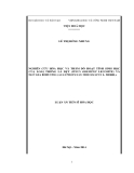
Figure 1: FLPA overview.
In this list, only the C55 is a low-power processor. This DSP is currently widely used in mobile devices, associated to the ARM7 or ARM9 in OMAP chips. The next generation of mobile devices however will inevitably require more power- ful processing capabilities, which will imply more complex processors. Indeed, the C55 is already aided by video co- processors for 2.5 G/3G applications. More complex DSPs will be used, like the C67/64/62, or low-power versions of these architectures (it is remarkable the C64 has already co- processors included in it). In this paper, we are presenting a methodology that was successfully applied, not only on the C55 and ARM7, but also on the more complex architectures of the C67/64 and 62. We thereby demonstrate the applica- bility of our methodology upon a large class of architectures, and we also guarantee that it will still be usable with the fu- ture generations of processors. In accordance with this idea, we also present some interesting applications of the method- ology not only on the C55, but also on the other processors for which we have developed a power model.
Provided that the power model of the processor is avail- able, there is no need for owning the processor itself to es- timate its consumption, nor for any specific development tool, since it is not even necessary to have the code com- piled. Thus, given an algorithm, a fast and cheap compari- son of different processors is possible. It is also possible to compare different algorithms, or different ways of writing an algorithm for a given application. The designer can locate which parts of the program are the most consuming, and fo- cus his/her optimization effort on these parts. Our method takes into account another very important parameter for the power consumption: the memory mapping. Indeed, the de- signer can place the data in external or internal memory, and can choose the internal bank where the data is stored. The place of data has a very strong impact on the consumption, and the designer is able to try and compare different data mappings with the help of our tool.
2. MODEL DEFINITION the architectural parameters. Algorithmic parameters indicate the activity level between every functional block in the pro- cessor (parallelism rate, cache miss rate, etc.). Architectural parameters depend on the processor configuration which is explicitly defined by the programmer (clock frequency, data mapping, etc.). Then, it is necessary to find how the func- tional blocks’ consumption varies with the parameters’ val- ues. We make the parameters vary with the help of elemen- tary assembly programs elaborated to stimulate each block or subblock separately. The variations of the processor’s supply current are measured on an evaluation board. A curve fitting of the graphical representation of these variations finally per- mits to determine the consumption rules by regression. The set of consumption rules for a given processor constitutes the so-called power model of this processor. The three main steps of the FLPA are summarized in Figure 1.
As stated before, we have developed a power model for five processors: the Texas Instrument C67, C64, C62, and C55, and the ARM7; and we have integrated these power models in our power and energy estimation tool SoftEx- plorer.
2.2. TI C62 and C67 power models 2.1. The functional-level power analysis Our estimation is based on the functional-level power anal- ysis (FLPA) of a processor. As stated before, the main advan- tage of this method compared to the ILPA is its simplicity, and the rapidity that it involves, both for building the model of a target, and for the estimation of a code. We recall here the FLPA general principle.
The TI C62 and C67 processors have complex architectures. Indeed, they both have a VLIW instructions set, a deep pipeline (up to 15 stages), and parallelism capabilities (up to 8 operations in parallel). Their internal program memory can be used like a cache in several modes, and an external memory interface (EMIF) is used to load and store data and program from the external memory [32]. Apart from the fact that the C62 operates in fixed point and the C67 in floating To perform a FLPA implies first to divide the processor in functional blocks. Functional blocks gather hardware re- sources that are activated together during a run. Obviously, relatively nonconsuming parts of the processor have to be discarded at that stage. Secondly, we have to find which fea- tures of the application impact the functional blocks’ activity, and thus the power consumption. These features are formal- ized in two sets of parameters: the algorithmic parameters and
Table 1: Sets of parameters.
PU
IMU FETCH/DP
Registers
Multiplexers
α
β
DC/ALU/MPY
CTRL
CTRL
τ
γ
1 − τ
1 − γ
DATA MEM.
PRG. MEM.
τ − ε
ε
MMU
DMA 1 EMIF
1
External memory
Parameters α β γ τ ε µ σ δ PSR W F
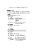
Figure 2: FLPA for the C62 and C67.
MM DM PM
C67 X X X X X — — — X X X X X —
C64 X X X — X X X X X X X X X —
C62 X X X X X — — — X X X X X —
C55 — X X — X — — — — X X X — X
ARM7 — — — — — — — — — — X X — —
2644 EURASIP Journal on Applied Signal Processing
point, they have very similar architectures. As a result, the functional analysis is identical for both of them, and leads to the block diagram in Figure 2.
whenever two data in the same internal memory bank are ac- cessed at the same time, the pipeline is stalled and that really changes the power consumption. Pipeline stalls are counted in the pipeline stall rate (PSR). Like τ, DM is included in the PSR in the power model. Table 1 summarizes the set of pa- rameters for the five considered processors.
Even if the C62 and C67 share the same set of parameters, the consumption rules that link these parameters to their actual power consumption are different. Indeed, the C62 is built upon a 0.25 µm process, and the C67 upon a 0.18 µm one. The supply voltage is 2.5 V for the C62, and 1.8 V for the C67. They therefore do not have identical static and dynamic power consumptions, and ought to have different consump- tion rules and hence, power models. Three blocks and five algorithmic parameters are iden- tified. The parallelism rate α assesses the flow between the FETCH stages and the internal program memory controller inside the IMU (instruction management unit). The process- ing rate β between the IMU and the PU (processing unit) represents the utilization rate of the processing units (ALU, MPY). The activity rate between the IMU and the MMU (memory management unit) is expressed by the program cache miss rate γ. The parameter τ corresponds to the ex- ternal data memory access rate. The parameter ε stands for the activity rate between the data memory controller and the direct memory access (DMA). The DMA may be used for fast transfer of bulky data blocks from the external to the internal memory (ε = 0 if the DMA is not used).
To the former algorithmic parameters four architectural parameters are added, that also strongly impact the proces- sor’s consumption: the clock frequency (F), the memory mode (MM), the data mapping (DM), and the data width during DMA (W). For these processors, no significant difference in power consumption was observed between an addition and a mul- tiplication, or a read and a write in the internal memory. Moreover, the effect of data correlation on the global power consumption appeared lower than 2%. More details on the consumption rules and their determination can be found in [31].
The influence of F is obvious. The C62 and C67 max- imum frequencies are respectively 200 MHz and 167 MHz, but the designer can tweak this parameter to adjust con- sumption and performances.
The memory mode MM illustrates the way the internal program memory is used. Four modes are available. All the instructions are in the internal memory in the mapped mode (MMM). They are in the external memory in the bypass mode (MMB). In the cache mode, the internal memory is used like a direct mapped cache (MMC), as well as in the freeze mode where no writing in the cache is allowed (MMF). Internal logic components used to fetch instructions (for instance tag comparison in cache mode) actually depend on the memory mode, and so the consumption.
2.3. TI C64 power model There are significant differences between the C64 and the C62/67 architectures. The internal program and data mem- ories have been replaced by two level-1 caches—the former memory modes have disappeared. A single level-2 cache is used both for the data and program. SIMD instructions can be used. The number of registers is doubled (2∗32 in place of 2∗16), as well as the number of DMA. Two coprocessors have been added (Viterbi + turbo decoder), and the C64 maxi- mum frequency goes from 600 MHz to 1 GHz. As a result, the power model is slightly different. As shown in Table 1, three new parameters were added. The miss rate for the level-1 data cache is µ. Even if µ = 0, the consumption may vary with the number of data reads or writes. In the C64, data are directly written into the level-2 cache and the power consumption is different for writes and reads. It is thus necessary to use two The data mapping impacts the processor’s consumption for two reasons. First, the logic involved to access a data in in- ternal or in external memory is different. Secondly, whenever a data has to be loaded or stored in the external memory, or
SoftExplorer: Power Estimation of a C Program for DSP and GPP 2645
different parameters: σ for the data read rate, and δ for the data write rate. The power consumption of the two copro- cessors has not been included in the power model yet. following principles. We will now explain these principles on the most complex architectures that we have studied yet, ac- cording to Table 1, the TI C62 and C67.
Before getting to the C-level, we will first observe what happens when an assembly program is executed on those processors. In the C6x, eight instructions are fetched at the same time. They form a fetch packet. In this fetch packet, operations are gathered in execution packets depending on the available resources and the parallelism capabilities. The parallelism rate α can be computed by dividing the number of fetch packets (NFP) by the number of execution packets (NEP) counted in the assembly code. However, the effective parallelism rate is drastically reduced whenever the pipeline stalls. Therefore, the final value for α must take the number of pipeline stalls into account. Hence, a pipeline stall rate (PSR) is defined, and α is computed as follows: 2.4. TI C55 power model The TI C55 is a low-power processor with a fixed-point ar- chitecture that can only execute two instructions in parallel; however, it only fetches one instruction at each clock cycle, and pipeline stalls never occur. Another characteristic of this processor is the possibility to automatically idle some parts of its architecture if unused. This is integrated in the param- eter PM (power management), which indicates the units in the sleep mode. The C55 internal program memory can be used in the same four modes as the C6x and it also contains a DMA and an EMIF. Because the C55’s architecture is less complex than the C6x’s, its power model has less parameters (see Table 1).
× (1 − PSR).
α = (1) NFP NEP
Identically, the PSR is considered to compute the process- ing rate β, with NPU the average number of processing units used per cycle (counted in the code), and NPUMAX the max- imum number of processing units that can be used at the same time in the processor (NPUMAX = 8 for the C6x):
×
× (1 − PSR).
β = (2) NPU NEP 1 NPUMAX
2.5. ARM7 power model The ARM7TDMI is the simplest processor that we have mod- eled yet. It has a scalar architecture and its internal program memory can be used in three modes (mapped, cache, and bypass). Previous works on the StrongArm have established that the power consumption essentially depends on the clock frequency and the supply voltage [33]. Our own consump- tion measurements on the ARM7TDMI have fully validated this trend: the power consumption variations corresponding to various programs are under 8% of the global consump- tion. No algorithmic parameter is then required to model the ARM7, as represented in Table 1.
The time necessary to complete the model of the C62 was about 30 days, and it took 15 days for the ARM7. It went faster for the C67 and C55 for we took benefit from the pre- vious study of the very similar C62 architecture. The use of an instruction-level method for such a complex architecture would have conducted to a prohibitive number of measure- ments. Indeed, with an ILPA approach, Bona et al. have char- acterized a simpler VLIW processor (the Lx) in 108 days [34].
3. ESTIMATION PROCESS
To determine α and β at the C-level, the three parameters NFP, NEP, and NPU must be predicted from the algorithm (instead of being counted in the assembly code). Indeed, even if our tool was initially designed to estimate the power con- sumption from an assembly code, the challenge here is to do it from the C program. It is clear that the prediction of NFP, NEP and NPU must rely on a model that anticipates the way the assembly code is executed on the target. This is actually related to the compiler behavior, and to the options chosen for the compilation. According to the processor’s architecture and with a little knowledge of the compiler, four prediction models were defined.
(i) The sequential model (SEQ) is the simplest one since it assumes that all the operations are executed sequentially. This model is only realistic for nonparallel processors. How- ever, it provides the absolute minimum bound of the algo- rithm’s power consumption.
(ii) The maximum model (MAX) corresponds to the case where the compiler fully exploits all the architecture possibil- ities. With this model, we assume that the maximum number of operations executable in parallel in a superscalar processor are indeed executed in parallel. In the C6x, 8 operations can be done in parallel; for example 2 loads, 4 additions, and 2 multiplications, in one clock cycle. This model gives a max- imum bound of the consumption. It will be also referred to as the “FULL parallel” model.
(iii) The minimum model (MIN) is more restrictive than the previous model since it assumes that load instructions, 3.1. Prediction models To compute the power consumption of an application, it is necessary to determine the parameters which are used in the target’s power model. To get the energy consumption, we will see later how to evaluate the execution time of the algorithm on the target. The process of finding the values of an applica- tion’s parameters gets difficult as the number of parameters in the power model increases. It is very simple for the ARM7 where only the frequency and memory mode are needed, but more difficult with the other processors. Determining the ar- chitectural parameters is straightforward since they are fixed by the programmer, or dependant on the architecture. To find the value of the algorithmic parameters implies a more precise knowledge of the processor’s behavior. However, the parameters we have proposed are general enough to be used for any pipeline and/or superscalar architecture when neces- sary, and are extracted from the application according to the
Table 2: Prediction models for the example.
α = β
EP2
EP3
EP4
Model EP1 MAX 2LD MIN 1LD DATA 2LD
2LD, 4OP 1LD 1LD
— 1LD 1LD, 4OP
— 1LD, 4OP —
0.5 0.25 0.33
2646 EURASIP Journal on Applied Signal Processing
3.2. Pipeline stalls As stated before, the pipeline stall rate PSR is needed to com- pute the values of the parameters α and β. To determine the PSR, we must evaluate the number of cycles where the pipeline is stalled (NPS) and divide it by the total number of cycles for the program to be executed (NTC):
PSR = . (3) NPS NTC
Pipeline stalls have several causes:
(i) a delayed data memory access: if the data is fetched in external memory (related to ε) or if two data are ac- cessed in the same internal memory bank (related to the data mapping DM);
or store instructions, are never executed at the same time— indeed, it was noticed on the compiled code that all paral- lelism capabilities were not always fully exploited for these instructions, depending on the compilation options. This is especially the case when the compiler is settled to min- imize the size of the assembly code. The data mapping is analyzed in this case only to assess the right value for the PSR (see Section 3.2). This model will be also referred to as the “SIZE optimal” model. It will give a more realistic lower bound for the algorithm’s power consumption than the se- quential model.
(ii) a delayed program memory access: in case of a cache miss for instance (related to the cache miss rate γ), or if the cache is bypassed or freezed (related to the memory mode MM);
(iii) a control hazard, due to branches in the code: we choose to neglect this contribution because only data- intensive applications are considered.
As a result, NPS is expressed as the sum of the number of cycles for stalls due to an external data access NPSτ, for stalls due to an internal data bank conflict NPSBC, and for stalls due to cache misses NPSγ:
NPS = NPSγ + NPSτ + NPSBC. (4) (iv) At last, the data model (DATA) refines the prediction for load and store instructions. The only difference from the MAX model is that it allows parallel loads and stores only if they involve data from different memory banks. In the C6x, for instance, there are two banks in the internal data memory which can be accessed in one clock cycle. It is thus possible to load two data in one cycle if one data is in the first bank, and the other data in the second one. The place of a data in the memory is found in the data mapping file, which, as before, will be also used to determine the PSR (Section 3.2). Such a behavior is observed when the compiler is settled to minimize the execution time of the code. This model will be also referred to as the “TIME optimal” model.
The prediction is performed by applying those models on all the program. As illustration, we present below a simple example:
For (i=0; i<512; i++) {Y=X[i]*(H[i]+H[i+1]+H[i-1])+Y;} Whenever a cache miss occurs, the cache controller, via the EMIF, fetches a full instruction frame (containing 8 in- structions) from the external memory. The number of cy- cles needed depends on the memory access time Taccess. As a result, where NFRAME is the number of frames causing a cache miss,
(5) NPSγ = NFRAME × Taccess.
Similarly, the pipeline is stalled during Taccess for each data access in the external memory. That gives, with NEXT being the number of data accesses in external memory,
(6) NPSτ = NEXT × Taccess.
In this loop nest, there are 4 loads (LD) and 4 other op- erations (OP): 1 multiplication and 3 additions. In our ex- ample, Y is stored in a register inside the processor. Here, our 8 operations will always be gathered in one single fetch packet, so NFP = 1. Because no NOP operation is involved, NPU = 8 and α and β parameters have the same value. In the SEQ model, instructions are assumed to be executed se- quentially. Then NEP = 8, and α = β = 0.125. Results for the other models are summarized in Table 2. X and H are supposed to be in distinct memory banks.
A conflict in an internal data bank is resolved in only one clock cycle. So, NPSBC is merely the number of bank conflicts NCONFLICT:
NPSBC = NCONFLICT. (7)
Of course, realistic cases are more elaborated: the param- eters prediction is done for each part of the program (loops, subroutines, etc.) for which local values are obtained. The global parameters values, for the complete C source, are com- puted by a weighted averaging of all the local values. Along with the global consumption, we indicate in SoftExplorer the consumption of every loop in the code (Section 4). Such an approach permits to spot “hot points” in the program. In the case of data-dependent algorithms, a statistic analysis may be performed to get those values (see Section 3.4). So, to calculate the PSR, we need the number of external data accesses NEXT, the number of internal data bank con- flicts NCONFLICT, and the number of instruction frames that involve cache misses NFRAME ((3), (4), (5), (6), and (7)). Those three numbers are directly extracted from the
Table 3: Relative error at the assembly level.
Maximal error Average error
C64 4.3% 2.6%
C62 4% 2.5%
C67 6% 2.4%
C55 2.5% 1.4%
ARM7 8% —
SoftExplorer: Power Estimation of a C Program for DSP and GPP 2647
assembly code when the estimation is performed at the as- sembly level. It is however remarkable that the two numbers NEXT and NCONFLICT can also be determined directly from the C program. Indeed, they are related to the data mapping which is actually fixed by the programmer by means of explicit compilation directives associated to the C sources, and only taken into account by the compiler during the link- age. The data mapping is integrated in the power model through the configuration parameter DM, which stands for the data mapping file. from the assembly code to obtain the former results at the as- sembly level, and the values that we can predict from the C program, according to our prediction models. In Table 4, the values of the power model parameters extracted from the as- sembly code, and from the C code assuming the DATA pre- diction model, are presented. We did not include the pre- dictions for the other prediction models since they provide higher and lower bounds that are naturally farther from the extracted value. For these applications, γ = 0 since the whole code is contained in the internal program memory, and ε = 0 since the DMA is not used. The PSR measured value (PSRm), obtained with the help of the TI development tool, is used for estimation at the assembly level (but the calculated value could be used as well). The average error between the pre- dicted (PSR) and the measured (PSRm) pipeline stall rates is 3.2%. It never exceeds 5.5% which indicates the PSR predic- tion accuracy.
External data accesses are fully taken into account through NEXT which participates in the calculation of the PSR. This is why the external data access parameter τ is said to be “included in the PSR” in the sets of parameters given in Table 1.
The power consumption of the algorithm is then esti- mated from the parameters that we have predicted from the C program. The relative error between the estimation and the measured consumption for the TI C62 at F = 200 MHz is given in Table 5. Results are given for the four prediction models at the C-level. We recall in the ASM column the pre- cision obtained at the assembly level.
Of course, the SEQ model gives the worst results since it does not take into account the architecture possibilities (par- allelism, several memory banks, etc.). In fact, this model was developed to explore the estimation possibilities without any knowledge about the architecture of the targeted processor. It seems that such an approach cannot provide enough accu- racy to be satisfying.
It is remarkable that, for the LMS in the bypass mode, ev- ery model overestimates the power consumption with close results. This exception can be explained by the fact that, in this marginal memory mode, every instruction is loaded from the external memory and thus pipeline stalls are dom- inant. As the SEQ model assumes sequential operations, it is the most accurate in this mode.
The number of instruction frames that involve cache misses NFRAME, as well as the cache miss rate γ, can be de- termined statically if the memory mode MM is mapped, by- pass, and freeze, or dynamically in cache mode. The assem- bly code size (with the total number of instruction frames) is needed for comparison with the cache size; a compilation is necessary. In this case, it is not possible to predict NFRAME at the C-level. However, since the assembly code for digital signal processing applications generally fits in the program memory of the processors, γ is most of the time equal to zero (as well as NFRAME). Whenever NFRAME and γ are not known in the early step of the design process, SoftExplorer will provide the designer with consumption maps to guide him through the code writing, as shown in Section 4.1 [35]. The number of DMA accesses can be determined from the assembly code or from the C program. Indeed, accesses to the DMA are explicitly programmed. The programmer knows exactly the number of DMA accesses; it is therefore easy to calculate the DMA access rate ε without compilation. It is computed by dividing the number of DMA accesses by the total number of data accesses in the program. For all the other algorithms, the MAX and the MIN mod- els always respectively overestimate and underestimate the application power consumption. Hence, the proposed mod- els need a restricted knowledge of the processor’s architec- ture; but they guaranty to bound the power consumption of a C algorithm with reasonable errors. 3.3. Estimation versus measures
The DATA model is the most accurate since it provides a maximum error of 8% against measurements. After compi- lation, the estimation can be performed at the assembly level where the maximum error is decreased to 3.5%.
The accuracy of our power and energy estimation at the as- sembly level has already been investigated [30]. For each of the five processors in our library of models, the power esti- mation was performed on a set of various algorithms—FIR filter, LMS filter, discrete wavelet transform (DWT) with dif- ferent image sizes, fast Fourier transform (FFT) 1024 points, enhanced full-rate (EFR) Vocoder for GSM, and MPEG-1 decoder. The power consumption was also measured for all these algorithms and processors. The relative errors between measures and estimations are reported Table 3.
Eventually, the estimation possibilities at the C-level are summarized. According to the results obtained with the SEQ model, it seems unrealistic to determine precisely the power consumption without any knowledge about the tar- geted processor. A coarse grain prediction model, includ- ing only the architecture possibilities in terms of parallelism, number of processing units, and so forth, provides the max- imum and minimum bounds of the algorithm’s power con- sumption with an average error of 7.3% and 15.2%, respec- tively. The fine grain prediction model, with both elementary Our aim in this section is to demonstrate the precision of power estimation at the C-level. We first perform some com- parisons with the values for α, β, and PSR that were extracted
Table 4: C-level parameters prediction versus ASM-level parameters extraction.
Configuration
Application
Assembly level β
α
PSRm
α
C-level β
PSR
MM
DM
FIR FFT LMS-1 LMS-2 DWT-1 (64 ∗ 64) DWT-2 (64 ∗ 64) DWT-3 (512 ∗ 512) EFR MPEG
MMM MMM MMB MMC MMM MMM MMM MMM MMM
INT INT INT INT INT EXT EXT INT INT
0.492 0.099 — 0.625 0.362 0.0915 0.088 0.594 0.706
0 0.64 0.93 0.25 0.027 0.755 0.765 0.225 0.108
0.454 0.08 0.029 0.483 0.287 0.0723 0.0695 0.472 0.715
0.5 0.119 — 0.76 0.365 0.105 0.1 0.669 0.682
0.5 0.113 0.0312 0.475 0.324 0.0932 0.089 0.479 0.568
0 0.604 0.95 0.24 0.0269 0.713 0.726 0.219 0.09
Table 5: C-level power estimation versus measurements.
Application
2648 EURASIP Journal on Applied Signal Processing
FIR FFT LMS-1 LMS-2 DWT-1 DWT-2 DWT-3 EFR MPEG
Measurements P(W) 4.5 2.65 4.97 5.66 3.75 2.55 2.55 5.07 5.83
In the case of dynamic loops, the number of iterations is not known in advance. SoftExplorer takes into account the algorithm’s dynamic behavior thanks to pragma directives added to the program: the user indicates a probability for the control structures (if, then, else, etc.) and the dynamic loops. A 50% probability is assumed whenever a pragma is miss- ing. A dynamic profiling may be necessary; specific analysis tools are usable for this purpose. The user could also give the maximum limit for the number of iterations to get a maxi- mum for the execution time and energy. At last, SoftExplorer considers the delays for division and function calls, to further increase the precision in estimating the execution time.
Estimation vs. measure. (%) ASM SEQ MAX MIN DATA 5.5 2.3 −38 2.87 2.5 −10 2.8 1.4 3.5 6.4 −1.8 −50 4.7 1.9 −27 3.4 −0.2 −10 2.4 −1 −10.4 −2.8 −50 1.5 0.7 −54 −33 −8 4.2 13.5 27.8 1.8
5.5 −24.3 28.5 −1 2.8 2 6.4 −15.2 4.7 −13.2 3.4 −4.2 2.4 −4.7 11.1 −24 10 8.3
Average errors
4. SOFTEXPLORER
4.1. Prediction types
information on the architecture and the data placement, of- fers a very accurate estimation with a maximum error of 8% against measurements.
3.4. Execution time prediction
A great part of the job for determining the execution time was already done for the PSR. In the previous section, we have indeed determined the number of pipeline stalls to- gether with their duration. The only remaining thing to do is to add the number of cycles for executing the program to the number of cycles where the pipeline is stalled, and to divide by the processor’s frequency. In fact, the algorithm is parsed loop by loop, and the data mapping is analyzed, to determine the number of memory conflicts which leads to the PSR.
All the previous estimations were performed with the help of SoftExplorer (v 5.0). SoftExplorer includes 17 000 lines of code and is written in C. When SoftExplorer is started, a configuration menu appears where it is possible to choose whether estimations will be performed at the C-level or at the assembly level. It is then necessary to choose the targeted processor’s power model among those available. As stated be- fore, there are currently 5 power models included (C67, C64, C62, C55, ARM7, though only the C62’s power model is pro- vided in the demo version). The input file (C code in our case, but could be also ASM code or PP-preprocessed file) is also indicated here. The data mapping file ought to be writ- ten in the same directory as the input file. Depending on the chosen power model, a configuration page for the C-level es- timation appears. In the case of the C6x and the C55, the pre- diction model (SEQ, MIN, DATA, MAX) must be indicated, together with the processor’s frequency. The memory mode (mapped, cache, freeze, bypass) is required for the C67, C62, and the C55. The prediction type has to be chosen as well. There are three prediction types.
We have estimated the execution time for the previously presented applications and compared it with the value given by the TI’s development tool: CodeComposer. This value is exact, for CodeComposer, after compilation, traces the as- sembly code on the evaluation board. We have then com- puted the energy from the estimated power consumption and execution time, and compared it with the energy com- puted from the measured power consumption and execution time. Errors less than 1% are observed. For example, the er- ror for the MPEG-1 decoder presented in the following sec- tion is 0.6%. Coarse prediction. There is no need for any further infor- mation from the user. The C code is parsed and the power consumption is computed with different values for γ and PSR from 0 to 100%. The result is a curve, or an area, dis- played on the “C curves results” or the “C area results” page.
)
W m
( r e w o P
)
4.2 3.8 3.4 3 2.6 2.2
90
0
10
20
30
40
50
60
70
80
90 100
W m
70
PSR (%)
30
( r e w o P
SoftExplorer: Power Estimation of a C Program for DSP and GPP 2649
m iss r ate
5.5 5 4.5 4 3.5 3 2.5
10
50 a c h e
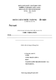
Figure 3: C curve: the power is a function of PSR (here) or γ.
C
0 10 20 30 40 50 60 70 80 90100
Pipeline stall rate
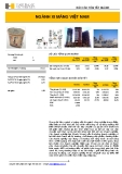
Figure 4: C area: the power is a function of PSR and γ.
Table 6: Power estimation in coarse prediction.
Pmax/Pmin (mW)
Mapped 4400/2200
Cache 5592/2353
Freeze 5690/2442
Bypass 5882/5073
Indeed, if the memory mode is bypass or mapped, then γ = 0, only the PSR varies, and a curve is computed. If the memory mode is cache or freeze, both the PSR and γ vary, and an area is drawn. These curves and areas are what we called consump- tion maps. The interest of the coarse prediction is to allow an estimation of an algorithm’s power consumption very early in the design process. Indeed, even if the data mapping is not settled (the data mapping is not considered in this mode), the programmer can have an idea of the power consumption, choose the processor, compare different algorithms, and be guided in the optimizations to be conducted on the code.
The power repartition in every functional part of the pro- cessor is also given (Figure 5). The DMA unit consumes no power for it is not used in this application. It is remarkable that a great part (47.4%) of the power consumption is due to the clock. The “loops” page display the power consumption, execution time, and α and β values, for each loop (Figure 6). These results are also presented in the form of a chronogram on the “graphics” page (Figure 7). The power consumption per functional part is also indicated on this graph. In the cache or freeze mode, the variations of the power consump- tion with γ are given on the “C curve” page.
Fine prediction. In this mode, the data mapping file is used to determine the data access conflicts (internal and ex- ternal) for each loop in the code. If γ = 0, which is the case for a large number of DSP applications, these conflicts permit to determine, for every loop, the precise number of pipeline stalls (i.e., the PSR) and the execution time. This local knowledge of every parameter in the power model of the target permits to compute, for each loop, the power con- sumption, the execution time, and the energy consumption. An accurate optimization of each portion of the code can be conducted that way.
An exact prediction is possible when the exact values for γ, PSR, and Texe are known. In our example, the TI’s devel- opment tool gives, after compilation, γ = 0, PSR = 0.2, and Texe = 40 microseconds. The power and energy estimations are displayed on the “results” page. The “loops” and “graph- ics” pages display local values for α, β, and the power con- sumption, assuming that pipeline stalls and cache misses are equally scattered in the algorithm. Exact prediction. The execution time, the cache miss rate, and the pipeline stall rate are no more predicted by SoftEx- plorer, but are instead provided by the user. They can be ob- tained with the help of the targeted processor’s development tools (e.g., TI’s CodeComposer for the C6x). C-level profilers can also be used for an estimation of the execution time.
For the ARM7, only the memory mode, operating fre- quency, and execution time are needed. There is no more need for distinct prediction models, nor for the three predic- tion types. Indeed, we measured that the program itself has only a slight influence on the consumption (see Section 2.5). To model the code, as well as the compiler, is therefore point- less. The estimation is performed directly from the parame- ters provided by the user.
4.2. Estimation time and complexity reduction
We show, on an example, the results that can be ob- tained with the three prediction types above. The applica- tion is the MPEG-1 decoder from MediaBench. Estimation is performed first in the coarse mode for the C62. Figure 3 shows the evolution of the power consumption P with the PSR (memory mode is mapped). The maximal value for P is 4400 mW when PSR = 0%, and its minimal value is 2200 mW for PSR = 100%. Figure 4 shows the evolution of the power consumption with both the PSR and γ (mem- ory mode is cache). This time, the max/min values for P are 5592/2353 mW. It can be observed that for the same PSR, the power consumption is always lower in the mapped mode. Table 6 indicates the max/min power consumption for the four memory modes.
A fine prediction takes into account the data mapping. In the mapped or bypass mode, the global power and energy consumptions are presented on the “results” page, with the execution time and the global values of parameters α and β. The time for SoftExplorer to parse a code and to perform an estimation is smaller at the C-level than at the assembly level. At the C-level, indeed, there is no need for compila- tion or a dynamic profiling. The C program has much less lines than the assembly code, and the overall process is faster even if it involves a little more computation to evaluate the consumption against the prediction model. At the assembly level, the estimation time varies from 3 seconds for an FIR
Table 7: Data mappings.
Mapping
a
b
c
e
f
1 2 3 4
EXT B0 B0 B0
EXT B0 B1 B1
EXT B0 B0 B2
EXT B0 B1 B3
EXT B0 B0 B4
2650 EURASIP Journal on Applied Signal Processing
5. APPLICATIONS
Figure 5: The “results” page also gives the power repartition.
Figure 6: The “loops” page presents the results for each loop.
×102
5.1. Influence of the data mapping
50 45 40 35 30 25 20 15 10 5 0
0
2
4
6
8
10 12 14 16 18 20 22 24 26
×102
We demonstrate on a simple example the influence of the data mapping on the power consumption and execution time. The algorithm that we use as a testbench manipulates at the same time 3 images of size 100 × 100 (a, b, c) and 2 vectors of size 10 (e, f) in 3 successively and differently imbri- cated loop nests. For the images and vectors are manipulated at the same time, their placement in memory has a strong influence on the number of access conflicts, and thus on the number of pipeline stalls. We show here that it is very quick and easy to try different placements, and to reach an optimal data mapping with the help of SoftExplorer. The four dif- ferent mappings that we tried are presented in Table 7. The results provided by SoftExplorer are presented in Table 8.
PLocale clock power PLocale fetch power PLocale processing unit power
Figure 7: A graphical display of the consumption per loop.
In the first mapping, all the data structures are placed in the external memory (EXT). As a result, there are as much external accesses as accesses to the memory, and for every access, the pipeline is stalled (during 16 cycles for the C6x). The relation between parameters α and β and the power con- sumption is obvious. When the pipeline is stalled, the num- ber of instructions that the processor executes in parallel (α) and the processing rate (β) decrease. As a result, the power consumption of the processor is reduced, but the execution time is lengthened and the energy consumption increases.
In the second mapping, all the structures are placed in the same bank in the internal memory (B0). There will be as much conflicts as before, but this time, the conflicts are in- ternal. The C6x’s pipeline is stalled during one cycle in case of an internal conflict. As a result, the time necessary to re- solve all the conflicts, expressed in number of cycles, equals the number of conflicts itself.
1024 or an LMS 1024, to 10 seconds for a DWT 512 × 512. We have compared this time with the estimation time ob- tained with the tool SimplePower [? ], which works cycle by cycle at the architectural level [29]. SoftExplorer appears to be thousands of times faster, since SimplePower treats the FIR 1024 in 4360 seconds, the LMS 1024 in 24 700 seconds, and the DWT 512 × 512 in 14 2000 s. SoftExplorer is even faster at the C-level: the estimation time is less than 1 second for every application that we have tested.
The interest of the last mapping 4 is to give a minimum bound in term of number of conflicts since every structure in the algorithm is in a different bank. This solution will also give the higher power consumption and the smaller execu- tion time. Indeed, since the pipeline is never stalled, the pro- cessor is used at its maximal capacity. The third mapping, which is achievable with a C6x, is as good as mapping 4 since it does not yield any conflict.
5.2. Choosing a processor and its operating frequency Even if it is easy to obtain the power consumption and the execution time of an algorithm with SoftExplorer, to actually find the right processor and its operating frequency is not straightforward. Indeed, the global energy consumed by the application depends not only on the energy consumed when the algorithm is executed, but also on the energy consumed To work on the C code is much more convenient for the user. Firstly, the code is smaller and more readable. Sec- ondly, the number of lines to be studied is drastically reduced once hot spots are located in the algorithm. Indeed, we have spotted, in the applications presented above, the consuming loops, and compared their length with the whole code [35]. Only 13% of the whole code, which represents only 10 lines, was significant for the FFT, 37% (17 lines) for the DWT, 31% (37 lines) for the EFR, 14% (4 lines) for the LMS, and 2% (30 lines) for the MPEG.
Table 8: SoftExplorer results with different mappings.
α
β
Mapping 1 2 3 4
0.0015 0.333 0.5 0.5
0.008 0.167 0.25 0.25
Texe (ms) 9.108 0.414 0.276 0.276
Current (mA) 870 1378 1644 1644
Power (mW) 2174 3444 4109 4109
Energy (mJ) 19.81 1.426 1.134 1.134
Conflicts 27 601 27 601 0 0
Tconflicts 441 616 27 601 0 0
Power
Pexe
) J (
l a b o
Active
l g
E
Pidle
4.5E − 5 4E − 5 3.5E − 5 3E − 5 2.5E − 5 2E − 5 1.5E − 5 1E − 5 5E − 6 0E + 0
0
50
150
200
Idle
100 F (MHz)
Time
Figure 9: Energy versus frequency for the C55.
Texe
Tconstraint
Figure 8: Power consumption and timing constraint.
) J (
SoftExplorer: Power Estimation of a C Program for DSP and GPP 2651
l a b o
l g
E
(cid:1)
(cid:2) .
when the processor is idle:
1.8E − 4 1.6E − 4 1.4E − 4 1.2E − 4 1E − 4 8E − 5 6E − 5 4E − 5 2E − 5 0E + 0
0
50
150
200
100 F (MHz)
Figure 10: Energy versus Frequency for the C62.
(8) Eglobal = Pexe × Texe + Pidle × Tconstraint − Texe
(cid:4) .
Figure 8 illustrates this equation. The timing constraint Tconstraint is the maximum bound for the execution time. Over this limit, the application’s data rate is not respected. Basically, if the frequency is high, the execution time is small and the active power (Pexe) increases. The idle time also in- creases with the frequency. On the other hand, as long as the execution time is lower than the timing constraint, it seems possible to slow down the processor to decrease Pexe. So, is it better to operate with a high or a low frequency? In fact, it actually depends on the application. C67. This minimum is 0.076 mJ for the C62 and 0.021 mJ for the C67, hence, the best processor/frequency couple among those two would be the C67 at 40 MHz. The shape of these two global energy curves is predictable when (8) is rewritten as
(cid:3) Tconstraint −
(10) Eglobal = (KF + C) × N F + K (cid:2)F × N F
= 1.01 ms.
We pursue a little farther the analysis with our preceding example, the MPEG-1 decoder (Section 4). This algorithm treats 4 macroblocs of a QCIF image in one iteration. A QCIF image (88 × 72) contains 396 macroblocs. Given a data rate of 10 images/s, the timing constraint is
× 4 396
(9) Tconstraint = 1 10
In this expression, Pexe is replaced with a dynamic term (KF), and a static one (C), while Texe is trivially replaced by N/F, where N is the number of cycles for one iteration. Pidle is given by the constructor as a product of F. When (10) is de- veloped, an F term and a 1/F term appear, and that explains the curves’ shape.
Then we use SoftExplorer to compute, at different fre- quencies, the execution time, power, and energy consumed by one iteration of the algorithm. Finally, we calculate with (8) the global energy consumed by the application at these frequencies. The results are presented in Figures 9, 10, and 11, respectively for the C55, C62, and the C67.
The two last curves (Figures 10 and 11) present a min- imum that gives the optimal operating frequency for this application: about 20 MHz for the C62 and 40 MHz for the Whenever Pidle does not vary with the frequency, it may be replaced with a constant term in (10), which, when de- veloped, includes only a 1/F term. The resulting curve does not present a minimum anymore; this is the case for the C55. For this processor, the frequency that gives the lower global energy consumption is the higher possible (200 MHz). How- ever, since the energy consumption is almost the same at 100 MHz, this last frequency will be preferred for it implies a
2652 EURASIP Journal on Applied Signal Processing
) J (
l a b o
l g
E
3E − 5 2.5E − 5 2E − 5 1.5E − 5 1E − 5 5E − 6 0E + 0
0
50
150
200
100 F (MHz)
Figure 11: Energy versus frequency for the C67.
caches (C64), and the floating-point VLIW (C67). Moreover, very important phenomena like pipeline stalls, cache misses, and memory accesses are taken into account.
To be able to perform an estimation at the assembly level, it was necessary to define two models: a model for the pro- cessor and a model for the algorithm. The model for the pro- cessor represents the way the processor’s consumption varies with its activity. The model for the algorithm links the algo- rithm with the activity it induces in the processor. Indeed, we showed that an algorithm has some intrinsic features like the parallelism rate or the processing rate.
lower power consumption: cooling devices will be lighter in this case. In fact, the global energy consumption for the C55 at 100 MHz is 0.015 mJ. As a result, the C55/100 MHz couple is definitely better than the two preceding.
We did not represent the wake-up time on Figure 8. In fact, we measured that this wake-up time is very small be- fore the execution time of the algorithm, and that the en- ergy consumption involved is negligible. Moreover, to avoid waking-up at each iteration, it is preferable to process a whole image with no interruption, and then to idle the processor until the next image. This decreases again the energy contri- bution of the waking-up. Of course, this can only be done if the application can bare a latency of one image. In a situa- tion where the wake-up time Twu could not be neglected, it is still possible to evaluate the global energy. Assuming that Twu is counted in processor’s cycles and that the wake-up power Pwu is proportional to the frequency F, one can write (with A and B constants)
(11) Pwu = B × F, Twu = A × 1 F ,
At the C-level, a third model is necessary: a model for the compiler. Indeed, given an algorithm, the processor’s activity actually depends on the compiler behavior. A programmer can set different options in the compiler to give the assembly code different features. Basically, the code can be optimized for performance (as fast as possible), or for size (as small as possible). Our model for the compiler is what we called the prediction model. We defined four prediction models. The DATA (TIME optimal) and MIN (SIZE optimal) mod- els represent the former compiler behaviors: respectively op- timization for performance and optimization for size. The MAX (FULL parallel) model gives a maximum bound for the power consumption and represents a situation where all the processing resources of the processor would be used rest- lessly. The SEQ (SEQuential) model stands for a situation where operations are executed one after the other in the pro- cessor. That gives an absolute minimum bound for the power consumption. In the case of the two first prediction models, the data mapping was taken into account. Indeed, we have demonstrated that the number of external accesses and the number of memory conflicts are directly related to the pro- cessor’s processing and parallelism rates, and to the pipeline stall rate (PSR), which have a great impact on the final power consumption and execution time. and the wake-up energy Ewu is a constant too:
(12) Ewu = Pwu × Twu = A × B.
As a result, the curves that give the global energy in func- tion of the frequency are shifted from the value of Ewu. The method to find the best processor and frequency remains the same.
6. CONCLUSION
We have developed a tool, SoftExplorer, which integrates our five power models, and can perform estimation both at the assembly and at the C-level. For DSP applications, and with elementary informations on both architecture and data placement, our C-level power estimation method provides accurate results together with the maximum and minimum bounds of the algorithm’s power consumption. The precision of SoftExplorer was evaluated by comparing estimations with measures for several representative DSP applications. The precision varies slightly from a processor to the other. For the C62, the maximal/average errors are 4/2.5% at the assembly level, and 8/4.2% at the C-level. This definitely demonstrates the possibility of performing an accurate power estimation of a C-algorithm.
We exhibit the influence of the data mapping and show how to use SoftExplorer to optimize the consumption and to reduce the complexity by focusing only on the most con- suming loops in the code. When the cache miss rate and/or pipeline stall rate are not defined, a consumption map al- lows to verify if the application constraints are respected. We present a methodology to determine the best proces- sor/frequency couple, for a given application. SoftExplorer is used to estimate the algorithm’s power consumption and We have introduced a new method for estimating the power and energy consumption of a DSP application directly from the C program. This method is build upon the functional- level power analysis (FLPA), which we designed initially to estimate the consumption from the assembly code. The ad- vantages of FLPA against instruction-level methods are a shorter delay to obtain a model of a processor, smaller time to achieve the estimation, and the ability to deal easily with complex architectures. Indeed, we have demonstrated our methodology on a wide range of architectures from the very simple general-purpose RISC processor (ARM7) to the more and more complex DSPs: the low-power (C55), the fixed- point VLIW (C62), the fixed-point VLIW with L1 and L2
[14] W.-T. Shiue, S. Udayanarayanan, and C. Chakrabarti, “Data memory design and exploration for low-power embedded systems,” ACM Transactions on Design Automation of Elec- tronic Systems, vol. 6, no. 4, pp. 553–568, 2001.
[15] Mentor Graphics Corporation: The EDA Technology Leader,
[Online]. Available: http://www.mentor.com/.
[16] Synopsys Corporation: EDA Solutions and Services, [Online].
SoftExplorer: Power Estimation of a C Program for DSP and GPP 2653
Available: http://www.synopsys.com/.
[17] D. Brooks, V. Tiwari, and M. Martonosi, “Wattch: a frame- work for architectural-level power analysis and optimiza- tions,” in Proc. 27th International Symposium on Computer Ar- chitecture (ISCA ’00), pp. 83–94, Vancouver, BC, Canada, June 2000.
execution time on several targets and at different frequencies. We show that the global energy consumed by the application depends on the frequency. With the timing constraint, the processor’s idle period of time is determined and the global energy computed. The frequency which yields the lowest consumption is adopted. The winning processor/frequency couple has the lowest energy consumption.
Future works include the development of new power models for the ARM9, the PowerPC, and the OMAP. A generic memory model will be added to include the external memory consumption in our power estimation. Power and energy estimation will be investigated at the system level.
[1] T. Hauser, “Convergence of two different worlds,” Electronic
[18] M. J. Irwin, M. Kandemir, N. Vijaykrishnan, and W. Ye, “The design and use of simple power: a cycle accurate energy esti- mation tool,” in Proc. 37th IEEE Conference on Design Automa- tion (DAC ’00), pp. 340–345, Los Angeles, Calif, USA, June 2000.
Design Europe, February 2003.
[2] H. Baaker, “Powering up the mobile phone,” Speech Technol-
ogy Journal, November/December 2001.
[19] D. Brooks, P. Bose, and M. Martonosi, “Power-performance simulation: design and validation strategies,” in ACM SIG- METRICS Performance Evaluation Review, 2004.
[3] S. Cordova, “Power management solutions for multimedia terminals,” in Proc. Batteries 2001 Conference, Paris, France, April 2001.
[20] D. Brooks, P. Bose, V. Srinivasan, M. K. Gschwind, P. G. Emma, and M. G. Rosenfield, “New methodology for early- stage, microarchitecture-level power-performance analysis of microprocessors,” IBM Journal of Research and Development, vol. 47, no. 5/6, 2003.
[4] M. Valluri and L. John, “Is Compiling for performance == compiling for power?” in Proc. the 5th Annual Workshop on Interaction between Compilers and Computer Architectures INTERACT-5, Monterrey, Mexico, January 2001.
[5] A. Fraboulet and A. Mignotte, “Source code loop transforma- tions for memory hierarchy optimizations,” in Proc. the Work- shop on Memory Access Decoupled Architecture MEDEA, Inter- national Conference on Parallel Architectures and Compilation Techniques (PACT ’01), pp. 8–12, Barcelona, Spain, September 2002.
[21] V. Zyuban, D. Brooks, V. Srinivasan, et al., “ Integrated analy- sis of power and performance for pipelined microprocessors,” IEEE Trans. Comput., vol. 53, no. 8, pp. 1004–1016, 2004. [22] J. S. Hu, N. Vijaykrishnan, S. Kim, M. Kandemir, and M. J. Ir- win, “Scheduling reusable instructions for power reduction,” in Proc. IEEE Conference and Exhibition on Design, Automa- tion and Test in Europe (DATE ’04), vol. 1, pp. 148–153, Paris, France, February 2004.
[6] S. Singhai and K. S. McKinley, “A parameterized loop fusion algorithm for improving parallelism and cache locality,” The Computer Journal, vol. 40, no. 6, pp. 340–355, 1997.
[23] V. Tiwari, S. Malik, and A. Wolfe, “Power analysis of embed- ded software: a first step towards software power minimiza- tion,” IEEE Trans. VLSI Syst., vol. 2, no. 4, pp. 437–445, 1994. [24] B. Klass, D. Thomas, H. Schmit, and D. Nagle, “Modeling inter-instruction energy effects in a digital signal processor,” in Proc. the Power Driven Microarchitecture Workshop in In- ternational Symposium on Computer Architecture (ISCA ’98), Barcelona, Spain, 1998.
[7] J. Ramanujam, J. Hong, M. Kandemir, and A. Narayan, “Re- ducing memory requirements of nested loops for embedded systems,” in Proc. 38th IEEE Conference on Design Automation (DAC ’01), pp. 359–364, Las Vegas, Nev, USA, June 2001. [8] T. V. Achteren, G. Deconinck, F. Catthoor, and R. Lauwere- ins, “Data reuse exploration techniques for loop-dominated applications,” in Proc. IEEE Conference and Exhibition on De- sign, Automation and Test in Europe (DATE ’02), pp. 428–435, Paris, France, March 2002.
[25] S. Steinke, M. Knauer, L. Wehmeyer, and P. Marwedel, “An ac- curate and fine grain instruction-level energy model support- ing software optimizations,” in Proc. IEEE International Work- shop on Power And Timing Modeling, Optimization and Sim- ulation (PATMOS ’01), pp. 3.2.1–3.2.10, Yverdon-Les-Bains, Switzerland, September 2001.
[9] L. Benini and G. De Micheli, “System-level power optimiza- tion: techniques and tools,” ACM Transactions on Design Au- tomation of Electronic Systems, vol. 5, no. 2, 2000.
[26] G. Qu, N. Kawabe, K. Usami, and M. Potkonjak, “Function- level power estimation methodology for microprocessors,” in Proc. 37th IEEE Conference on Design Automation (DAC ’00), pp. 810–813, Los Angeles, Calif, USA, June 2000.
[10] C. H. Gebotys, “Utilizing memory bandwidth in DSP embed- ded processors,” in Proc. 38th IEEE Conference on Design Au- tomation (DAC ’01), pp. 347–352, Las Vegas, Nev, USA, June 2001.
[11] C. Kulkarni, C. Ghez, M. Miranda, F. Catthoor, and H. De Man, “Cache conscious data layout organization for embed- ded multimedia applications,” in Proc. IEEE Conference and Exhibition on Design, Automation and Test in Europe (DATE ’01), pp. 686–691, Munich , Germany, March 2001.
[27] L. Benini, D. Bruni, M. Chinosi, C. Silvano, V. Zaccaria, and R. Zafalon, “A Power modeling and estimation framework for VLIW-based embedded systems,” in Proc. IEEE Interna- tional Workshop on Power And Timing Modeling, Optimization and Simulation (PATMOS ’01), pp. 2.3.1–2.3.10, Yverdon-les- Bains, Switzerland, September 2001.
[12] P. Panda, F. Catthoor, N. D. Dutt, et al., “Data and memory optimization techniques for embedded systems,” ACM Trans- actions on Design Automation of Electronic Systems, vol. 6, no. 2, pp. 149–206, 2001.
[28] C. H. Gebotys and R. J. Gebotys, “An empirical comparison of algorithmic, instruction, and architectural power predic- tion models for high performance embedded DSP proces- sors,” in Proceedings of International Symposium on Low Power Electronics and Design (ISLPED ’98), pp. 121–123, Monterey, Calif, USA, 1998.
[13] F. Catthoor, K. Danckaert, C. Kulkarni, and T. Omns, Data Transfer and Storage (DTS) Architecture Issues and Exploration in Multimedia Processors, Marcel Dekker, NewYork, NY, USA, 2000.
[29] J. Laurent, N. Julien, E. Senn, and E. Martin, “Functional level power analysis: an efficient approach for modeling the power
REFERENCES
consumption of complex processors,” in Proc. IEEE Confer- ence and Exhibition on Design, Automation and Test in Europe (DATE ’04), vol. 1, pp. 666–667, Paris, France, February 2004. [30] N. Julien, J. Laurent, E. Senn, and E. Martin, “Power con- sumption modeling and characterization of the TI C6201,” IEEE Micro, vol. 23, no. 5, pp. 40–49, 2003, Special Issue on Power- and Complexity-Aware Design.
[31] J. Laurent, E. Senn, N. Julien, and E. Martin, “High level en- ergy estimation for DSP systems,” in Proc. IEEE International Workshop on Power And Timing Modeling, Optimization and Simulation (PATMOS ’01), pp. 311–316, Yverdon-les-Bains, Switzerland, September 2001.
2654 EURASIP Journal on Applied Signal Processing
Eric Martin is a Professor at the Univer- sity of South Brittany in Lorient, and Direc- tor of the LESTER Laboratory. His research interests focus on advanced electronic de- sign automation dedicated to real-time sig- nal processing applications, including sys- tem specification, high-level synthesis, in- tellectual property reuse, low-power design, systems on a chip, and platform prototyp- ing. He has a Ph.D. degree from the Univer- sity of Paris XI, France. He is a Member of the IEEE, of the IEEE Computer Society, and of the IEEE Circuits and Systems Society.
[32] TMS320C6x User’s Guide, Texas Instruments Inc., 1999. [33] A. Sinha and A. P. Chandrakasan, “JouleTrack - A web based tool for software energy profiling,” in Proc. 38th IEEE Confer- ence on Design Automation (DAC ’01), pp. 220–225, Las Vegas, Nev, USA, June 2001.
[34] A. Bona, M. Sami, D. Sciuto, C. Silvano, V. Zaccaria, and R. Zafalon, “Energy estimation and optimization of embedded VLIW processors based on instruction scheduling,” in Proc. 39th IEEE Design Automation Conference (DAC ’02), pp. 886– 891, New Orleans, La, USA, June 2002.
[35] E. Senn, N. Julien, J. Laurent, and E. Martin, “Power estima- tion of a C algorithm on a VLIW processor,” in Proceedings of Workshop on Complexity-Effective Design (WCED ’02) (in conjunction with the 29th Annual International Symposium on Computer Architecture (ISCA ’02)), Anchorage, Alaska, USA, May 2002.