
112 J. FOR. SCI., 56, 2010 (3): 112–120
JOURNAL OF FOREST SCIENCE, 56, 2010 (3): 112–120
In the Czech forest typology and geobiocoenology,
the term vegetation tier has been introduced as an
analogue of more general terms altitudinal vegeta-
tion zone or vegetation belt (see Zlatník 1976a). Al-
titudinal zonation of vegetation has been known for a
long time (Huggett, Cheesman 2002). Altitudinal
vegetation zones (or belts) have been recognized and
studied in many regions in the world (Ellenberg
1986; Hegazy et al. 1998; Hemp 2006; Zhang et
al. 2006). Vegetation tiers represent superstructural
units in both typological systems for forest and land-
scape classification in the Czech Republic. The first
one, the typological system of Forest Management
Institute (FMI) (Randuška et al. 1986; Viewegh et
al. 2003), finds its use mainly in forestry. The second
one is the system of geobiocoenological typology
(Buček, Lacina 2007) which is used to classify the
whole landscape. Both systems characterize poten-
tial vegetation rather than the actual one.
Zlatník (1976a) defined vegetation tiers as “the
connection of the sequence of differences in vegeta-
tion with the sequence of differences in the climate
of different altitude and exposure climate”. Ten
vegetation tiers were distinguished in the former
Czechoslovakia (Zlatník 1976b). The first eight
tiers (1–8) were named after main woody species
growing naturally in particular tiers under normal
soil water content (oak, beech-oak, oak-beech,
beech, fir-beech, spruce-fir-beech, spruce and dwarf
mountain pine vegetation tier). Vegetation tiers are
mapped based on the occurrence of plant bioindi-
cators, site altitude, slope orientation, and terrain
relief. The characteristics of vegetation tiers used
in geobiocoenological typology were described by
Buček et al. (2005), Buček and Lacina (2007).
Differences in the typological system of FMI were
described by Randuška et al. (1986). Holuša and
Holuša (2008) described the detailed character-
Supported by the Higher Education Development Fund, Project No. 1130/2008/G4, and by the Ministry of Education, Youth
and Sports of the Czech Republic, Project No. MSM 6215648902.
Application of digital elevation model for mapping
vegetation tiers
D. Volařík
Department of Forest Botany, Dendrology and Geobiocoenology, Faculty of Forestry
and Wood Technology, Mendel University in Brno, Brno, Czech Republic
ABSTRACT: The aim of this paper is to explore possibilities of application of digital elevation model for mapping
vegetation tiers (altitudinal vegetation zones). Linear models were used to investigate the relationship between vegeta-
tion tiers and variables derived from a digital elevation model – elevation and potential global radiation. The model
was based on a sample of 138 plots located from the 2nd to the 5th vegetation tier. Potential global radiation was com-
puted in r.sun module in geographic information system GRASS. The final model explained 84% of data variability and
employed variables were found to be sufficient for modelling vegetation tiers in the study area. Applied methodology
could be used to increase the accuracy and efficiency of mapping vegetation tiers, especially in areas where such task
is considered difficult (e.g. agricultural landscape).
Keywords: altitudinal vegetation zones; digital elevation model; linear models; vegetation tiers

J. FOR. SCI., 56, 2010 (3): 112–120 113
istics of the 3rd and the 4th vegetation tiers of the
north-eastern Moravia and Silesia. Air and soil tem-
perature, precipitation amount and its distribution
are considered to be the main direct factors influ-
encing the altitudinal vegetation zonation (Zlatník
1976b; Randuška et al. 1986).
Digital Elevation Model (DEM) contains infor-
mation both on altitude and topography. DEM is
considered to be the main prerequisite map for
spatial modelling in ecology (Guisan, Zimmer-
mann 2000). It determines the spatial resolution
of all derived maps, such as a map of slope, aspect,
and curvatures. DEM has been used as a source of
variables in numerous vegetation studies (e.g. Del
Barrio et al. 1997; Gottfried et al. 1998; Guisan
et al. 1998).
Three types of environmental variables or gradi-
ents can be recognized: indirect gradients, direct
gradients, and resource gradients (Austin 1980).
Elevation, slope, and aspect represent indirect en-
vironmental gradients. The derivation of variables
which have a more obvious influence on vegetation
may help to elucidate the relations studied (Austin
et al. 2006). The aspect is a typical example which
is inapplicable to some analyses in its original ex-
pression (359° and 1° are far outlying values albeit
the real difference in exposure is only slight). The
aspect can be substituted by radiation which has
a more obvious impact on vegetation, and in addi-
tion, it includes the influence of slope steepness and
possibly other variables (terrain shading, latitude).
Relatively simple formulae for radiation have been
introduced e.g. by McCune and Keon (2002). More
sophisticated models are incorporated in geographic
information systems (Šúri, Hofierka 2004; Pierce
Jr. et al. 2005).
The aim of presented paper is to explore possibili-
ties of using DEM for mapping vegetation tiers. DEM
is considered to be a useful tool for transferring the
knowledge of vegetation tiers from easily classifi-
able sites to the sites that are not easily classifiable
(e.g. large areas of non-native spruce monocultures,
agricultural land).
MATERIAL AND METHODS
Study area
The study area is located in the Zlín Region,
around the towns of Valašské Klobouky and Bru-
mov-Bylnice, and between the towns of Uherský
Brod, Luhačovice, and Bojkovice. Both sites cover
an area of approximately 10,000 ha in total. The area
lies within the Natural Forest Area Bílé Karpaty and
Vizovické vrchy (Plíva, Žlábek 1986). The altitude
ranges from 250 to 835 m a.s.l., with Průklesy being
the highest point. The soil parent material is sand-
stone and claystone of flysch layers (Chlupáč 2002).
The main soil type is Cambisol (Czech Geological
Survey 2003). Mean annual temperature (for the
period 1961–2000) ranges from 6 to 9°C, depending
on the altitude; mean annual precipitation varies
from 650 to 1,000 mm (Tolasz 2007).
Data collection
Phytosociological relevés were recorded in 2007 to
2008 using standard methods. Relevés were record-
ed in square geobiocoenological plots (20 × 20 m),
located in 2007 in various forest stands so as to cap-
ture the variability of vegetation. In 2008, the plots
were supplemented by plots selected by a stratified
random sampling design, in which altitude, aspect,
predominant tree species, and historical land-use
were considered. Trees were classified into several
vertical strata using Zlatník’s adjusted scale; the
cover for each species in the layer was determined
using the abundance-dominance scale (Zlatník
1976b). A total of 200 relevés were recorded. All
relevés were classified into the system of geobio-
coenological typology (Buček, Lacina 2007). The
relevés from the nutrient-poor soils were excluded
(trophic range A and AB according to Buček,
Lacina 2007), as well as the relevés from the tufa
mounds and waterlogged sites.
The locations of phytosociological relevés were
determined by GPS. In 2007, GPS receiver Garmin
GPSMAP 76S was used; recorded data were trans-
ferred to GRASS GIS (GRASS Development Team
2009). In 2008, Trimble Juno ST GPS receiver with
ArcPad 7.1.1 (ESRI) software and Trimble GPSCor-
rect 2.40 (Trimble) extension was employed. Data
were transferred to ArcGIS 9.2 (ESRI) with Trimble
GPS Analyst 2.10 (Trimble) extension. Phytoso-
ciological relevés were stored in TURBOVEG 2.75
program (Hennekens, Schaminee 2001).
Determining vegetation tiers
Geobiocoenological plots were classified into veg-
etation tiers of the geobiocoenological classification
system (Buček et al. 2005; Buček, Lacina 2007)
while the species combination of herb-, shrub- and
tree-layer, altitude and aspect were taken into ac-
count. Bioindicator values of plant species associ-
ated with vegetation tiers were used according to
Zlatník (1963) and Ambros and Štykar (2001).
At low altitude sites, relatively few relevés were re-

114 J. FOR. SCI., 56, 2010 (3): 112–120
corded, therefore 7 supplementary plots were estab-
lished. Supplementary plots were similarly classified
into vegetation tiers although no phytosociological
relevés were performed.
Digital elevation model and derived maps
DEM was interpolated from contour lines using
the RST (regularized spline with tension) method.
Contour line data were obtained from the Fundamen-
tal Base of Geographic Data of the Czech Republic
(ZABAGED) provided by the Czech Office for Sur-
veying, Mapping and Cadastre. Klimánek (2006)
found ZABAGED as the best generally available
source of elevation data in the Czech Republic. Maps
of slope, aspect, and annual sum of potential global
radiation (hereinafter referred to as potential global
radiation) were derived. All the above-mentioned
calculations were processed within GRASS GIS en-
vironment. Potential global radiation was calculated
in r.sun module. This module can be used to compute
direct, diffuse and reflected solar radiation for a par-
ticular day in the year, based on latitude, type of sur-
face and atmospheric conditions (Hofierka, Šúri
2002; Neteler, Mitasova 2008). For the purposes
of analysis, global radiation was calculated as the sum
of direct and diffuse radiation; impact of atmospheric
conditions was omitted from the calculation, while
the effect of terrain shading was included. The resolu-
tion of raster maps was 5 m, except for the maps of
potential global radiation (10 m resolution).
Data analyses
The influence of the variables on the herb layer spe-
cies composition was evaluated by indirect ordina-
tion method – non-metric multidimensional scaling
(NMDS; using 2 dimensions) and by fitting the vari-
ables as vectors to the ordination plot. The influence
of DEM-derived variables (elevation, potential global
radiation, and slope steepness), vegetation tiers and
percent tree canopy cover was assessed. The smooth
surface for vegetation tiers was also fitted to the
ordination plot (using generalized additive models
– GAM). Before the analyses, data were edited using
the JUICE 6.5 (Tichý 2002) program – the nomen-
clature was unified and the data set was divided into
3 subsets for analyses. The first subset contained all
relevés in which at least 2 species per plot occurred
in the herb layer (188 relevés), the second subset
consisted of all records with at least 8 herb-layer
species (170 relevés), and the third subset included
all records with at least 14 herb-layer species (131 re-
levés). The species cover values were transformed
using square root transformation; data were stan-
dardized; Jaccard index of dissimilarity was used for
the purposes of NMDS. Statistical significance of the
impact of each variable was tested by permutation
tests; the impact of variables was compared using the
coefficient of determination (R2).
A linear model for vegetation tiers was developed,
using vegetation tiers determined by a field survey
as dependent variables, and elevation and potential
global radiation as independent variables. The model
was based on data from geobiocoenological plots in
which more than 14 herb layer species were found
and from supplementary plots (in total 138 plots).
The cross-correlation between elevation and poten-
tial global radiation was weak (R = –0.1471). Vegeta-
tion tiers represent an ordinal variable (values 2, 3, 4
and 5 in model area). However, when developing the
model they were considered as a continuous variable.
Model values are therefore continuous and the limits
between vegetation tiers had to be set for them. The
limits were set so as to achieve the minimum number
of plots differently classified by the model.
Comparison of model vegetation tiers and
vegetation tiers obtained from the Regional
Plans of Forest Development (RPFD)
The map of model vegetation tiers was compared
with the map of vegetation tiers classified by the
typological system of FMI obtained from the Re-
gional Plans of Forest Development (RPFD, Forest
Management Institute in Brandýs nad Labem 2003).
The comparison was carried out only for forest land
within the boundaries of the study area. Error matrix
and the percentage of correctly classified pixels were
calculated in the GRASS GIS environment (about
error matrix e.g. in Campbell 2002).
RESULTS
Classification of plots into vegetation tiers
based on a field survey
Out of 131 geobiocoenological plots in which at
least 14 herb layer species were found, 5 were classi-
fied into the 2nd vegetation tier, 50 into the 3rd, 62 into
the 4th, and 14 into the 5th tier. All supplementary
plots were classified into the 2nd vegetation tier. The
second vegetation tier is found at the lowest eleva-
tions (240–380 m a.s.l.), the 3rd tier at elevations of
330–550 m, the fourth at 500–740 m, and the fifth
above 650 m (Fig. 1). Plots located in the third and
fourth tiers are evenly distributed along the gradi-
ent of potential global radiation, plots in the fifth

J. FOR. SCI., 56, 2010 (3): 112–120 115
tier have mainly shady aspect with lower potential
global radiation, while plots in the second tier have
mainly sunny aspect (with higher potential global
radiation) (Fig. 2).
Variability of vegetation
Phytosociological relevés were classified into
9 groups of geobiocoene types after removing
those from the nutrient-poor soils, tufa mounds
and waterlogged sites. In the 2nd vegetation tier
there were Fagi-querceta typica, Fagi-querceta
aceris, Fagi-querceta tiliae, in the 3rd vegetation
tier Querci-fageta typica, Querci-fageta aceris,
Querci-fageta tiliae, in the 4th ve-getation tier
Fageta typica, Fageta aceris and in the 5th ve-
getation tier Abieti-fageta typica and Abieti-fageta ace-
ris inferiora. Phytosociological relevés were re-
Vegetation tier
2 3 4 5
Altitude (m a.s.l.)
800
700
600
500
400
300
Vegetation tier
2 3 4 5
Potential global radiation (MWh.m–2 per year)
2.0
1.6
1.2
Table 1. Coefficients of determination (R2) and significances based on permutation tests (1,000 permutations) for
variables fitted as vectors to the NMDS ordination. (The analysis was performed for 3 subsets of data: subset I included
all phytosociological relevés in which at least 2 species per plot occurred in the herb layer, subset II (at least 8 herb-layer
species per plot) and subset III (at least 14 herb-layer species per plot))
Variable R2 (significance)
subset I (≥ 2 species) subset II (≥ 8 species) subset III (≥ 14 species)
Cover of tree layer 0.0898 (***) 0.2210 (***) 0.3335 (***)
Elevation 0.2457 (***) 0.3247 (***) 0.4062 (***)
Slope 0.0638 (**) 0.0551 (**) 0.0391 (.)
Radiation 0.1706 (***) 0.1487 (***) 0.1486 (***)
Vegetation tiers 0.2380 (***) 0.3168 (***) 0.4670 (***)
Significance levels: ***α = 0.001. **α = 0.01. *α = 0.05. (.) α = 0.1
Fig. 2. Box-and-whisker plots showing the distribution of po-
tential global radiation in vegetation tiers determined through
field survey. Center line and outside edge (hinges) of each box
represent the median and range of inner quartile around the
median; vertical lines on the two sides of the box (whiskers)
represent values falling within 1.5 times the absolute value
of the difference between the values of the two hinges; circle
represents outside values
Fig. 1. Box-and-whisker plots showing the distribution of eleva-
tion in vegetation tiers determined through field survey. Center
line and outside edge (hinges) of each box represent the median
and range of inner quartile around the median; vertical lines on
the two sides of the box (whiskers) represent values falling within
1.5 times the absolute value of the difference between the values
of the two hinges; circle represents outside values
116 J. FOR. SCI., 56, 2010 (3): 112–120
NMDS1
–1.0 –0.5 0.0 0.5
NMDS2
0.6
0.4
0.2
0.0
–0.2
–0.4
–0.6
–0.8
2nd vegetation tier
3rd vegetation tier
4th vegetation tier
5th vegetation tier
4
3.5
3
2.5
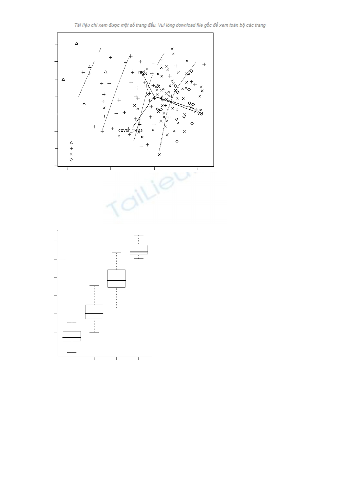
Fig. 3. NMDS ordination plot for subset of phytosociological relevés with more than 14 species. Only species from herb layer are
used for ordination. Environmental variables (rad – potential global radiation, elev – elevation), cover of tree layer (cover_trees) and
vegetation tiers (VS) are fitted as vectors on the ordination. Vegetation tiers are fitted also as surface using GAM (grey isolines)
Fig. 4. Box-and-whisker plots showing the distribution of model
values of vegetation tiers in vegetation tiers determined through
field survey. Center line and outside edge (hinges) of each box
represent the median and range of inner quartile around the
median; vertical lines on the two sides of the box (whiskers)
represent values falling within 1.5 times the absolute value
of the difference between the values of the two hinges; circle
represents outside values
Vegetation tier
2 3 4 5
Model values
5.0
4.5
4.0
3.5
3.0
2.5
2.0
corded in forest stands with the near natural tree
species composition (mainly with Quercus petraea,
Fagus sylvatica, Carpinus betulus and Abies alba)
as well as in forest stands hardly influenced by
human activities (Picea abies and Pinus sylvestris
monocultures).
Influence of variables on vegetation
Elevation, potential global radiation, tree canopy
cover and vegetation tiers are variables which signifi-
cantly influence the herb layer species composition.
Significances and coefficients of determinations
(R2) for variables fitted to NMDS ordination for all
subsets of plots are shown in Table 1. Elevation and
potential global radiation fitted as vectors to NMDS
ordination are significant with P value < 0.001.
R2 for elevation is highest in the subset of plots with at
least 14 species of herb layer (R2 = 0.4062) and lowest
in the subset of plots with at least 2 species of herb
layer (R2 = 0.2457). R2 for potential global radiation is
almost the same for all 3 analyzed subsets. Another
DEM-derived variable is slope. Its influence on the
herb layer species composition is lower; it is not
statistically significant (at α = 0.05) for the subset of
records with at least 14 herb layer species per plot. The
variable ‘tree canopy cover’ is significant with P value
< 0.001 and it has the highest influence in the subset of
records with at least 14 herb layer species per plot.


%20--%3e%3cdefs%3e%3cstyle%3e%20.st0%20{%20fill:%20%23fff;%20}%20.st1%20{%20fill:%20%237800fa;%20}%20%3c/style%3e%3c/defs%3e%3cpath%20class='st1'%20d='M117.78,12.18H43.11c2.9,3.47,4.65,7.94,4.65,12.82,0,5.6-2.3,10.66-6.01,14.29h76.02l7.22-13.56-7.22-13.56Z'/%3e%3cg%3e%3cpath%20class='st0'%20d='M53.58,26.17h-.59v-1.46h.59v-4.96h2.83c1.78,0,2.67.94,2.67,2.82v5.76c0,1.87-.89,2.81-2.67,2.81h-2.83v-4.96ZM55.36,21.37v3.34h1.1v1.46h-1.1v3.34h1.01c.61,0,.91-.37.91-1.1v-5.93c0-.74-.3-1.1-.91-1.1h-1.01Z'/%3e%3cpath%20class='st0'%20d='M65.99,31.14h-1.8l-.31-2.07h-2.19l-.31,2.07h-1.64l1.82-11.39h2.62l1.82,11.39ZM65.28,18.04c-.25.46-.51.77-.75.94-.21.15-.47.22-.79.22-.26,0-.57-.07-.92-.22l-.38-.15c-.14-.05-.26-.07-.37-.07-.3,0-.53.18-.71.54l-.91-.68c.25-.46.51-.77.75-.94.21-.14.48-.21.79-.21.26,0,.57.07.92.21l.38.15c.14.05.26.07.37.07.3,0,.53-.18.71-.54l.91.68ZM61.91,27.52h1.73l-.87-5.76-.87,5.76Z'/%3e%3cpath%20class='st0'%20d='M74.53,26.89v1.52c0,1.91-.89,2.86-2.67,2.86s-2.67-.95-2.67-2.86v-5.93c0-1.91.89-2.86,2.67-2.86s2.67.95,2.67,2.86v1.11h-1.69v-1.22c0-.75-.31-1.12-.93-1.12s-.93.37-.93,1.12v6.15c0,.74.31,1.11.93,1.11s.93-.37.93-1.11v-1.63h1.69Z'/%3e%3cpath%20class='st0'%20d='M81.4,31.14h-1.8l-.31-2.07h-2.19l-.31,2.07h-1.64l1.82-11.39h2.62l1.82,11.39ZM75.9,19.2l1.52-1.91h1.71l1.51,1.91h-1.61l-.76-.95-.75.95h-1.61ZM77.32,27.52h1.73l-.87-5.76-.87,5.76ZM83.1,15.99l-1.76,1.91h-1.26l1.17-1.91h1.86Z'/%3e%3cpath%20class='st0'%20d='M84.86,19.75c1.78,0,2.67.94,2.67,2.82v1.48c0,1.87-.89,2.81-2.67,2.81h-.85v4.28h-1.79v-11.39h2.64ZM84.01,21.37v3.86h.85c.58,0,.87-.36.87-1.08v-1.71c0-.71-.29-1.07-.87-1.07h-.85Z'/%3e%3cpath%20class='st0'%20d='M93.51,19.75c1.78,0,2.67.94,2.67,2.82v1.48c0,1.87-.89,2.81-2.67,2.81h-.85v4.28h-1.79v-11.39h2.64ZM92.66,21.37v3.86h.85c.58,0,.87-.36.87-1.08v-1.71c0-.71-.29-1.07-.87-1.07h-.85Z'/%3e%3cpath%20class='st0'%20d='M98.8,31.14h-1.79v-11.39h1.79v4.88h2.03v-4.88h1.83v11.39h-1.83v-4.88h-2.03v4.88Z'/%3e%3cpath%20class='st0'%20d='M105.36,24.55h2.46v1.62h-2.46v3.34h3.09v1.63h-4.88v-11.39h4.88v1.63h-3.09v3.18ZM108.17,17.29l-1.76,1.91h-1.26l1.17-1.91h1.86Z'/%3e%3cpath%20class='st0'%20d='M112.2,19.75c1.78,0,2.67.94,2.67,2.82v1.48c0,1.87-.89,2.81-2.67,2.81h-.85v4.28h-1.79v-11.39h2.64ZM111.35,21.37v3.86h.85c.58,0,.87-.36.87-1.08v-1.71c0-.71-.29-1.07-.87-1.07h-.85Z'/%3e%3c/g%3e%3ccircle%20class='st1'%20cx='25'%20cy='25'%20r='20'/%3e%3cpath%20class='st0'%20d='M32.78,19.27c2.92,0,4.43,2.55,5.28,5.33l.71,2.17c.14.38-.33.75-.71.75h-5.61c.19-.33.24-.71.09-1.08l-.75-2.45c-.43-1.32-.99-2.64-1.79-3.77.75-.57,1.65-.94,2.78-.94h0ZM25,18.38c3.25,0,4.9,2.78,5.89,5.89l.76,2.45c.14.42-.33.8-.8.8h-11.69c-.42,0-.94-.38-.8-.8l.75-2.45c.99-3.11,2.64-5.89,5.89-5.89h0ZM25,11.35c1.74,0,3.11,1.37,3.11,3.11s-1.37,3.11-3.11,3.11-3.11-1.41-3.11-3.11,1.41-3.11,3.11-3.11h0ZM17.27,19.27c1.08,0,1.98.38,2.73.94-.8,1.13-1.37,2.45-1.74,3.77l-.8,2.45c-.14.38-.05.75.09,1.08h-5.56c-.42,0-.9-.38-.75-.75l.71-2.17c.9-2.78,2.41-5.33,5.33-5.33h0ZM17.27,12.91c1.51,0,2.78,1.27,2.78,2.83s-1.27,2.83-2.78,2.83-2.83-1.27-2.83-2.83,1.27-2.83,2.83-2.83h0ZM32.78,12.91c1.56,0,2.78,1.27,2.78,2.83s-1.23,2.83-2.78,2.83-2.83-1.27-2.83-2.83,1.27-2.83,2.83-2.83h0ZM27.07,28.56v.09c0,.57-.24,1.08-.61,1.46h0v.05c-.38.33-.9.57-1.46.57s-1.08-.24-1.46-.61h0c-.38-.38-.61-.9-.61-1.46v-.09h1.41v.09c0,.19.05.38.19.47v.05c.09.09.28.19.47.19s.38-.09.47-.19v-.05c.14-.09.24-.28.24-.47t-.05-.09h1.41ZM30.99,28.56v.09c0,1.65-.66,3.16-1.74,4.24-1.08,1.08-2.59,1.79-4.24,1.79s-3.16-.71-4.24-1.79l-.05-.05c-1.04-1.08-1.7-2.55-1.7-4.2v-.09h1.41v.09c0,1.27.47,2.4,1.27,3.25h.05c.85.85,1.98,1.37,3.25,1.37s2.4-.52,3.25-1.37c.85-.8,1.37-1.98,1.37-3.25v-.09h1.37ZM34.99,28.56v.09c0,2.78-1.13,5.28-2.92,7.07-1.79,1.79-4.29,2.92-7.07,2.92s-5.23-1.13-7.07-2.92c-1.79-1.79-2.92-4.29-2.92-7.07v-.09h1.41v.09c0,2.4.94,4.53,2.5,6.08,1.56,1.56,3.72,2.5,6.08,2.5s4.52-.94,6.08-2.5c1.56-1.56,2.5-3.68,2.5-6.08v-.09h1.41Z'/%3e%3c/svg%3e)