
96 DISCRETE-SIGNAL ANALYSIS AND DESIGN
adjust scaling factors (Chapter 1) as needed to assure “adequate” cover-
age and resolution of time and frequency. The smoothing and windowing
methods in Chapter 4 are helpful in reducing time and frequency require-
ments without deleting important data. This is where the “art” of approx-
imation and “practical” engineering get involved, and we delay the more
advanced mathematical considerations for consideration “down the road.”
Also, small quantities of noise can very quickly take us into the com-
plexities of statistical analysis. We are for the most part going to avoid
this arena because it is does not suit the limited purposes of this book.
For this reason we are going to be somewhat less than rigorous in some
of the embedded-noise topics to be covered. However, we will have brief
contacts that will give us a “feel” for these topics.
PROPERTIES OF A DISCRETE SEQUENCE
Expected Value of x(n)
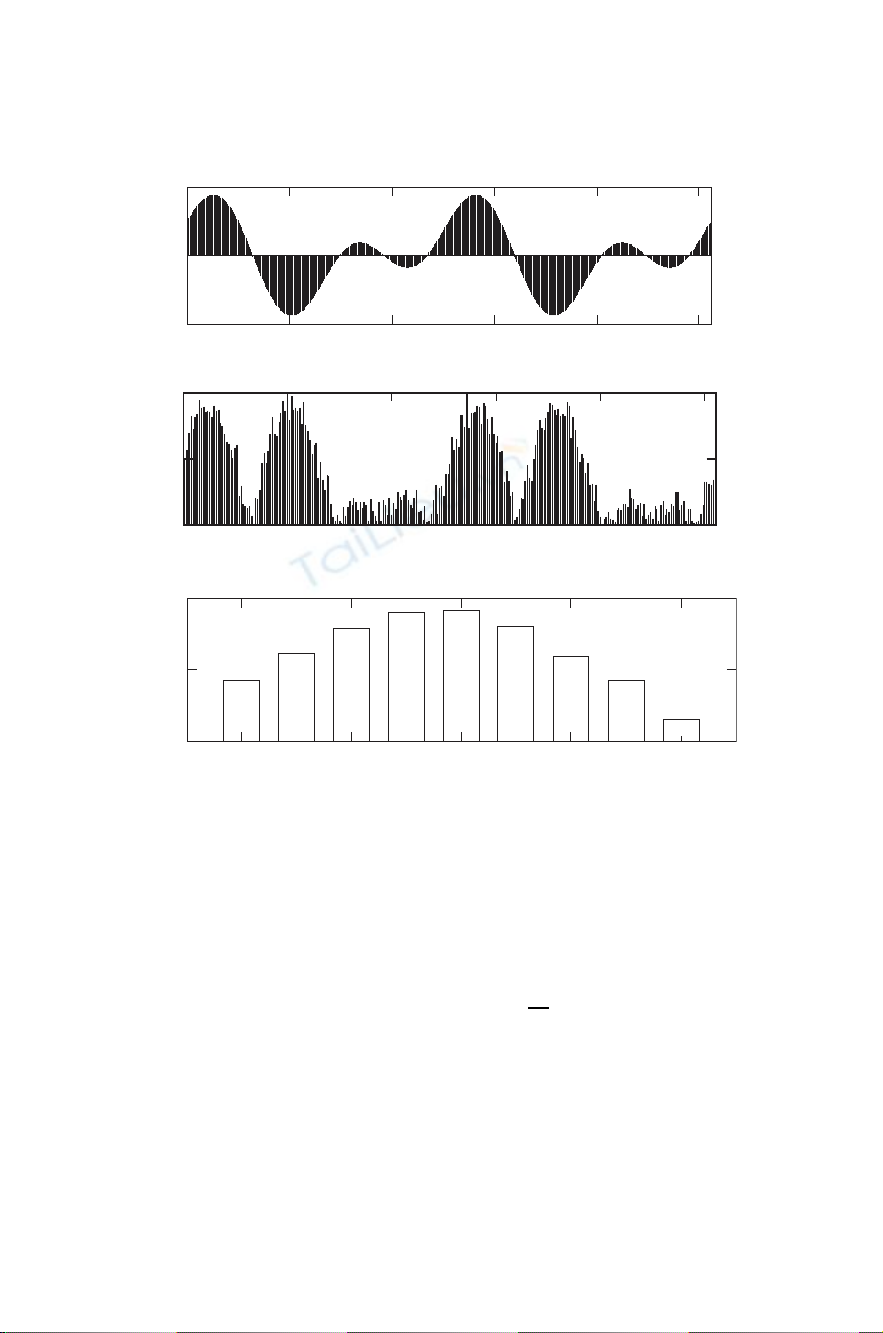
In Fig. 6-1a, a discrete time sequence (256 points) is shown from n=0
to N−1. The Þrst (positive) half is from 0 to N/2−1, and the second
(negative) half is from N/2 to N−1, as we saw in Figs. 1-1d and 1-2b.
ForaninÞnite x(n) sequence, the quantity E[x(n)], the statistical expected
value, also known as the Þrst moment [Meyer, 1970, Chap. 7], is
E[x(n)]=∞
n=−∞
x(n)p(x(n)) (6-1)
where p(x(n)istheprobability, from 0.0 to +1.0, of occurrence of a
particular x(n)ofaninÞnite sequence. In deterministic sequences from
0toN−1 such as Fig. 6-1a each x(n) is assumed to have an equal
probability 1/Nfrom 0 to N−1 of occurrence, the amplitudes of x(n)
can all be different, and Eq. (6-1) reverts to the time-average value x(n)
from 0 to N−1, which we have been calling the time-domain dc value,
and which is also identical to the zero frequency X(0) value for the X(k)
frequency-domain sequence. Note that the angular brackets in x(n)refer
to a time average. We have reasonably assumed that expected value and
PROBABILITY AND CORRELATION 97
−2
0
0
(a)
(b)
(c)
2
255
−0.4 −0.2 0 0.2 0.4
1
10
100
Noise count (vertical) vs. noise amplitude (horizontal) for 256 total counts
7
13
45 55 63
46
17
7
3
050 100 150 200 250
0
1
2
Figure 6-1 Signal without noise (a), with noise and envelope detected
(b), and a sample histogram of the envelope-detected noise alone (c).
time-average value are the same for a repetitive deterministic sequence
with little or no aliasing:
X(0)=E[x(n)]=x(n)= 1
N
N−1
n=0
x(n) (6-2)
all of which are zero in Fig. 6-1a.
Figure 6-1b introduces a small amount of additive noise voltage ε(n)
to each x(n), so called because each x(n) is the same as in Fig. 6-1a but
with noise ε(n) that is added to x(n), not multiplied by x(n) as it would
be in various nonlinear applications. The noise voltage itself, as found
98 DISCRETE-SIGNAL ANALYSIS AND DESIGN
dB
dB
Linear
Plot
0.4
0.3
0.2
0.1
0
s = 1
−5−4−3−2−1012345
−10 −8−6−4−20246810
0
−20
−40
−60
−80
−100
−120
0
−20
−40
−60
−80
−100
−120
−140
−4−3−2−101234
s = 2
s = 1
s = 2
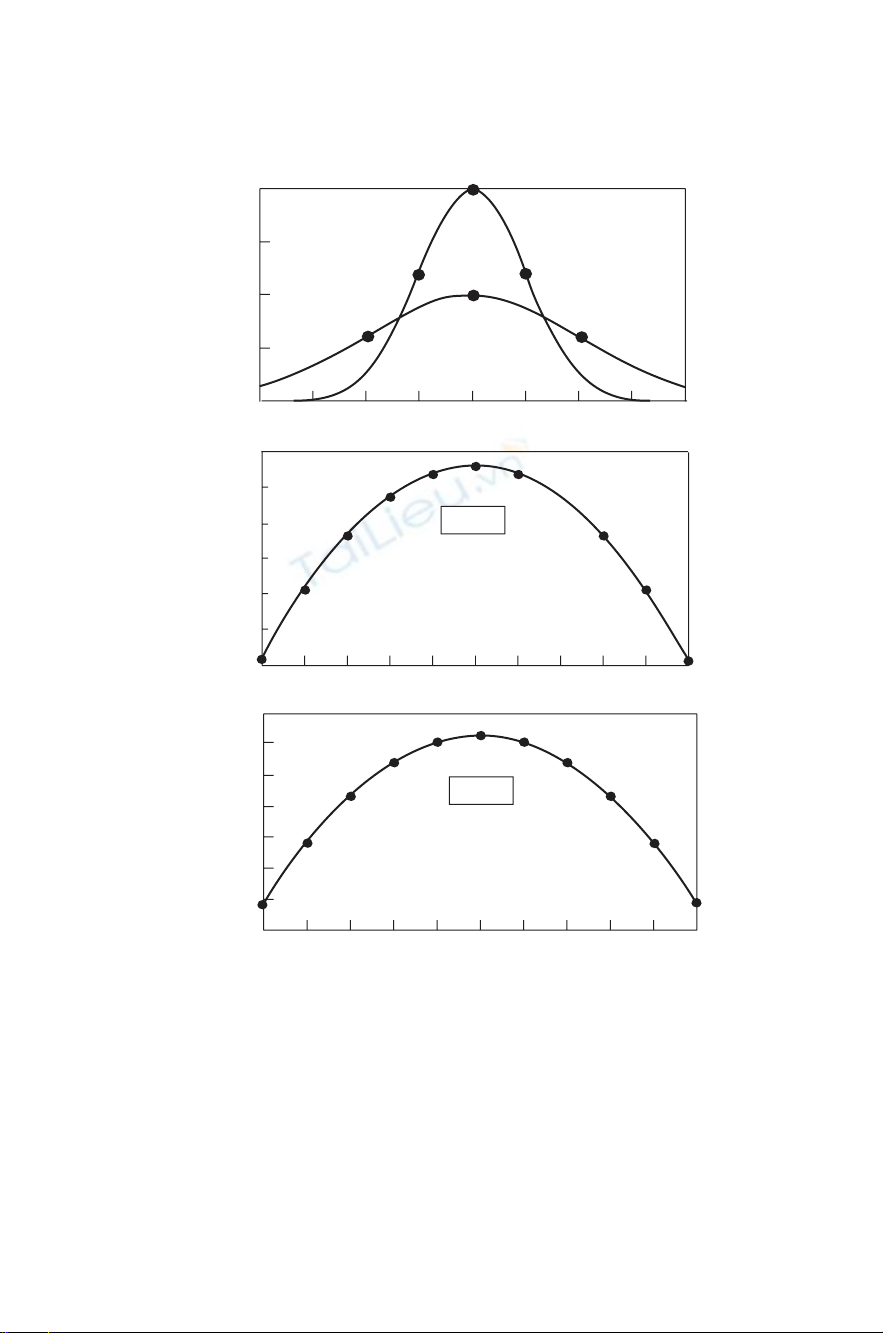
Figure 6-2 Normal distribution for σ= 1 and 2.
in communications systems, is assumed to have the familiar bell-shaped
Gaussian (also called) amplitude density function shown in the histogram
in Fig. 6-1c and in more detail in Figs. 6-2 and 6-3 [Schwartz, 1980,
Chap. 5]. See also Chapter 7 of this book for a more detailed discussion
of noise and its multiplication.

PROBABILITY AND CORRELATION 99
The noise has random amplitude. For this discussion, the signal plus
noise [x(n)+ε(n)] is measured by an ideal (linear) full-wave envelope
detector that delivers the value |x(n)+ε(n)|at each (n), where the vertical
bars imply the positive magnitude. In Fig. 6-1b the ε(n) noise voltage is
a small fraction of the signal voltage. In each calculation of the sequence
x(n) a new sequence εx(n) is also generated. Equation (6-3) Þnds the
positive magnitude of [x(n)+ε(n)].
E[|(x +ε)n|]≈|(x +ε)n| ≈ 1
N
N−1
n=0
[|(x +ε)n|] (6-3)
This is an example of the wide-sense stationary process, in which the
expected value and the time average of a very long single record or the
average of many medium-length records are the same and the autocorre-
lation value (discussed later in the chapter) depends only on the time shift
τ[Carlson, 1986, Chap. 5.1].
The contribution of the sequence ε(n) to the detector output is a ran-
dom variable that ßuctuates with each solution of Eq. (6-3). The histogram
approximation in Fig. 6-1c for one of the many solutions shows a set of
amplitude values of ε(n), arranged in a set of discrete values on the hor-
izontal scale, with the number of times that value occurs on the vertical
scale. The total count is always 256, one noise sample for each value
of nfrom 0 to 255. The count within each rectangle, divided by 256,
is the fraction of the total occurring in that rectangle. This is a sim-
ple normalization procedure that we will use [see also Schwartz, 1980,
Fig. A-9]. The averaging of a large number of these data records leads to
an ensemble average. A single very long record such as N=216 =65,536
using Mathcad is also a very good approximation to the expected value.
Average Power
The average power, also known as the expected value of x(n)2and also
as the time-average value x(n)2of the deterministic (no noise) sequence
in Fig. 6-1a is 1.00 W into 1.0 ohm, found in Eq. (6-4)
Pav =E[x(n)]2=x(n)2=1
N
N−1
n=0
x(n)2=1.00 W (6-4)

100 DISCRETE-SIGNAL ANALYSIS AND DESIGN
This includes any power due to a dc component in x(n), which in
Fig. 6-1a is zero. The power in the envelope-detected signal is also
1.00 W. The total power in both cases must be identical because this
ideal full-wave envelope detector is assumed to be 100% efÞcient. In Fig.
6-1b with added noise, the power is
Pav ≈1
N
N−1
n=0
[x(n) +ε(n)]2
≈1
N
N−1
n=0(x(n))2+2x(n)ε(n) +(ε(n))2(6-5)
≈1
N
N−1
n=0(x(n))2+(ε(n))2≈1.024 W (on average)
and the additional 0.024 W is due to noise alone.
In most situations, the expected value of the product [2x(n)ε(n)] is
assumed to be zero because these two are, on average, statistically inde-
pendent of each other. In this example with additive noise and full-wave
ideal envelope detection we will be slightly more careful. Comparing
noise and signal within the linear envelope detector, and assuming that
the signal is usually much greater than the noise, the noise and signal are,
as a simpliÞcation, in phase half of the time and in opposite phase half
of the time. P(n) can then be approximated as
P(n) ≈[x(n) +ε(n)]2=x(n)2+2x(n)ε(n) +ε(n)2
≈[x(n) −ε(n)]2=x(n)2−2x(n)ε(n) +ε(n)2(6-6)
average value of P(n) ≈x(n)2+ε(n)2
which is the same as Eq. (6-5).
Individual calculations of this product in Eq. (6-5) vary from about
+20 mW to about −20 mW, and the average approaches zero over many
repetitions. A single long record N=216 =65,536 produces about ±1.0
mW, and Pav ≈1.024 W.
The Pav result is then the expected value of signal power plus the
expected value of noise power. This illustrates the interesting and useful


![Giáo trình Thiết kế logo căn bản (Ngành Thiết kế đồ họa Trung cấp) - Trường Cao đẳng Xây dựng số 1 [Mới nhất]](https://cdn.tailieu.vn/images/document/thumbnail/2024/20240624/gaupanda039/135x160/3561719229819.jpg)

![Giáo trình Design thị giác (Thiết kế đồ họa Trung cấp) - Trường Cao đẳng Xây dựng số 1 [Mới nhất]](https://cdn.tailieu.vn/images/document/thumbnail/2024/20240624/gaupanda039/135x160/7481719229857.jpg)


![Giáo trình AutoCAD Pro Design: Phần 2 - Dương Đức Cảnh [Full]](https://cdn.tailieu.vn/images/document/thumbnail/2022/20221214/phuongnguyen0520/135x160/1030337256.jpg)
![Giáo trình AutoCAD Pro Design: Phần 1 - Dương Đức Cảnh [Hướng dẫn chi tiết]](https://cdn.tailieu.vn/images/document/thumbnail/2022/20221214/phuongnguyen0520/135x160/1724121258.jpg)