THE HILBERT TRANSFORM 131
0 16 32 48 64 80 96 112 128
0
−1
1
x(n)
n
(a)
N := 128 n := 0, 1.. N
k := 0, 1.. N
x(n) :=0
−1 if n>
1 if n> 0
0 if n=N
0 if n=
N
2
N
2
(
c
)
XH(k) :=−j⋅X(k) if k < N
2
N
2
0 if k=
N
2
j⋅X(k) if k>
0 163248648096112128
−1
−0.5
0
0.5
1
Im(X(k))
k
(b)
Imaginary
X(k) :=∑
N−1
n= 0
1
N
n
N
x(n)⋅exp −j⋅2⋅π⋅ ⋅k
⋅
Figure 8-1 Example of the Hilbert transform.
132 DISCRETE-SIGNAL ANALYSIS AND DESIGN
0 16 32 48 64 80 96 112 128
−1
−0.5
0
0.5
1
Re(XH(k))
k
Real
(d)
0 20 40 60 80 100 120
−4
−3
−2
−1
0
1
2
3
4
(xh(n))
x(n)
n
(f)
xh1(n) := 0.25⋅xh(n− 1) + 0.5⋅xh(n)+ 0.25⋅xh(n+ 1)
xh2(n) := 0.25⋅xh1(n− 1) + 0.5⋅xh1(n)+ 0.25⋅xh1(n+ 1)
(g)
−4
−3
−2
−1
0
1
2
3
4
0 20 40 60 80 100 120
xh2(n)
x(n)
n
(
h
)
(e)
xh(n) :=∑
N−1
k= 0
k
N
(XH(k))⋅exp j⋅2⋅π⋅ ⋅n
Figure 8-1 (continued)

THE HILBERT TRANSFORM 133
chapter we will continue to use DFT and IDFT and stay focused on the
main objective, understanding the Hilbert transform.
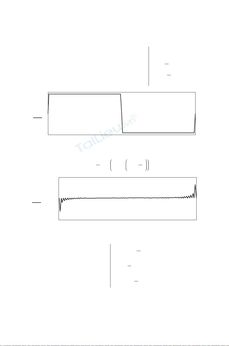
Why do the samples in Fig. 8-1f and h bunch up at the two ends and
in the center to produce the large peaks? The answer can be seen by
comparing Fig. 8-1b and d. In Fig. 8-1b we see a collection of (sine)
wave harmonics as deÞned in Fig. 2-2c. These sine wave harmonics are
the Fourier series constituents of the symmetrical square wave in Fig.
8-1a. In Fig. 8-1d we see a collection of ( −cosine) waves as deÞned
in Fig. 2-2b. These ( −cosine) wave harmonic amplitudes accumulate at
the endpoints and the center exactly as Fig. 8-1f and h verify. As the
harmonics are attenuated, the peaks are softened. The smoothing also
tends to equalize adjacent amplitudes slightly. The peaks in Fig. 8-1h rise
about 8 dB above the square-wave amplitude, which is almost always too
much. There are various ways to deal with this. One factor is that the
square-wave input is unusually abrupt at the ends and center. Smoothing
(equivalent to lowpass Þltering) of the input signal x(n), is a very useful
approach as described in Chapter 4. This method is usually preferred in
circuit design.
It is useful to keep in mind, especially when working with the HT,
that the quadrature of θ, which is θ±90◦, is not always the same thing
as the conjugate of θ. If the angle is +30◦, its conjugate is −30◦, but its
quadrature is +30◦±90◦=+120◦or −60◦. The HT uses θ◦±90◦.For
example, Fig. 8-1b shows +j0.5 at k =127. The HT multiplies this by +j
to get a real value of −0.5 in part (d) at k=127. This is a quadrature
positive phase shift at negative frequency k=127. A similar event occurs
at k=1. Also, at k=0andNthe phase jump is 180◦from ±jto ∓j,
and the same, although barely noticeable, at N/2. (Use a highly magniÞed
vertical scale in Mathcad.)
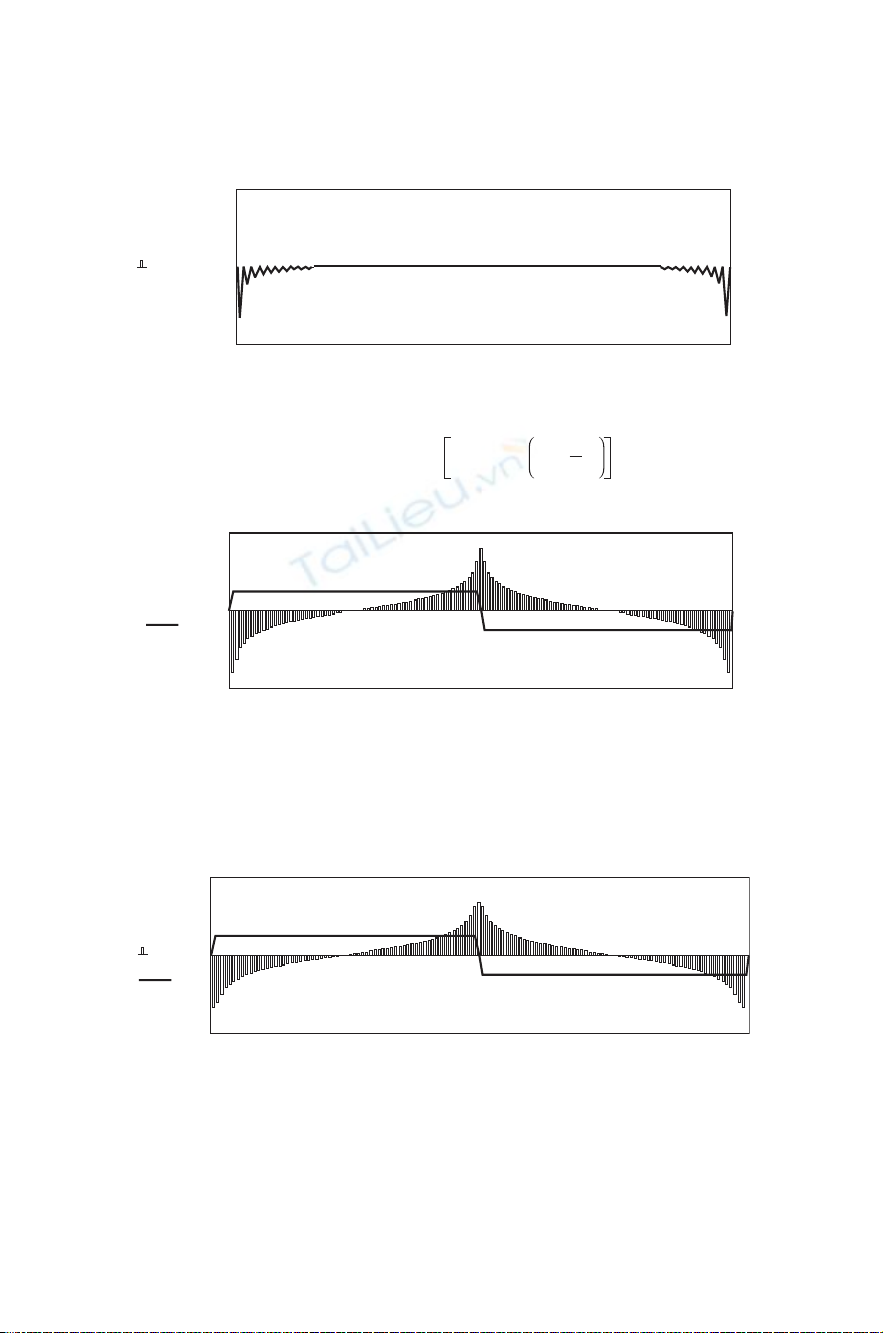
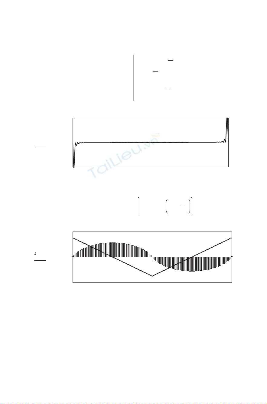
A different example is shown in Fig. 8-2. The baseband signal in
part (b) is triangular in shape, and this makes a difference. The abrupt
changes in the square wave are gone, the baseband spectrum (d) contains
only real cosine-wave harmonics, and the Hilbert transform (f) contains
only sine-wave harmonics. The sharp peaks in xh(n) that we see in
Fig. 8-1g disappear in Fig. 8-1h. However, for equal peak-to-peak ampli-
tude, the square wave of Fig. 8-1 has 4.8 dB more average power than
the triangular wave of Fig. 8-2. It is not clear what practical advantage

134 DISCRETE-SIGNAL ANALYSIS AND DESIGN
0 16324864
n
80 96 112 128
−4
−2
0
2
x(n)
−0.5
0.5
0
1
1.5
Re(X(k))
x(n):=
N:= 128 n:= 0, 1 .. Nk:= 0, 1 .. N
3 if n= 0
3− if n≥ 1
3 if n=N
(a)
(b)
0 16324864
k
80 96 112 128
(d)
(c)
∑
N−1
n= 0
X(k) :=1
Nx(n)⋅exp n
N
−j⋅2⋅π⋅ ⋅k
12·n
N
−9+ 12· if n >
n
N
N
2
⋅
Figure 8-2 Hilbert transform using a triangular waveform.
the triangular wave would have. The importance of peak amplitude limits
and peak power limits in circuit design must always be kept in mind.
BASIC PRINCIPLES OF THE HILBERT TRANSFORM
There are many types of transforms that are useful in electronics work. The
DFT and IDFT are well known in this book because they transform back
THE HILBERT TRANSFORM 135
xH(k):= −j⋅ X(k) if k<
0 if k=
1
0.5
0
(e)
N
2
j⋅ X(k) if k>N
2
N
2
−1
−0.5
4
−4
−3
−2
−1
0
1
2
3
0 16324864
k
(f)
(g)
80 96 112 128
02040
n
(h)
60 80 100 120
Im(XH(k))
x
(n)
Re(xh(n))
∑
N−1
n= 0
xh(n) :=(XH(k)⋅exp k
N
j⋅2⋅π⋅ ⋅k
Figure 8-2 (continued)
and forth between the discrete time-domain signal x(n) and the discrete
frequency-domain spectrum X(k).
Another very popular transform converts a linear differential equation
into a linear algebraic equation. For example, consider the differential


![Giáo trình Thiết kế logo căn bản (Ngành Thiết kế đồ họa Trung cấp) - Trường Cao đẳng Xây dựng số 1 [Mới nhất]](https://cdn.tailieu.vn/images/document/thumbnail/2024/20240624/gaupanda039/135x160/3561719229819.jpg)

![Giáo trình Design thị giác (Thiết kế đồ họa Trung cấp) - Trường Cao đẳng Xây dựng số 1 [Mới nhất]](https://cdn.tailieu.vn/images/document/thumbnail/2024/20240624/gaupanda039/135x160/7481719229857.jpg)