156 DISCRETE-SIGNAL ANALYSIS AND DESIGN
N := 8 n := 0,1.. N
VC := 1.5 IL := 1.0 R := 3 L := 1 C := 0.5
x(n) :=
VC
IL
if n = 0
T . +
0
1
L
−1
C
R
L
1
0
0
1
x(n− 1) if n > 0
0 0.1 0.2 0.3 0.4 0.5 0.6 0.7 0.8
0
0.3
0.6
0.9
1.2
1.5
V(C)
I(L)
x(n)0
x(n)1
n.T
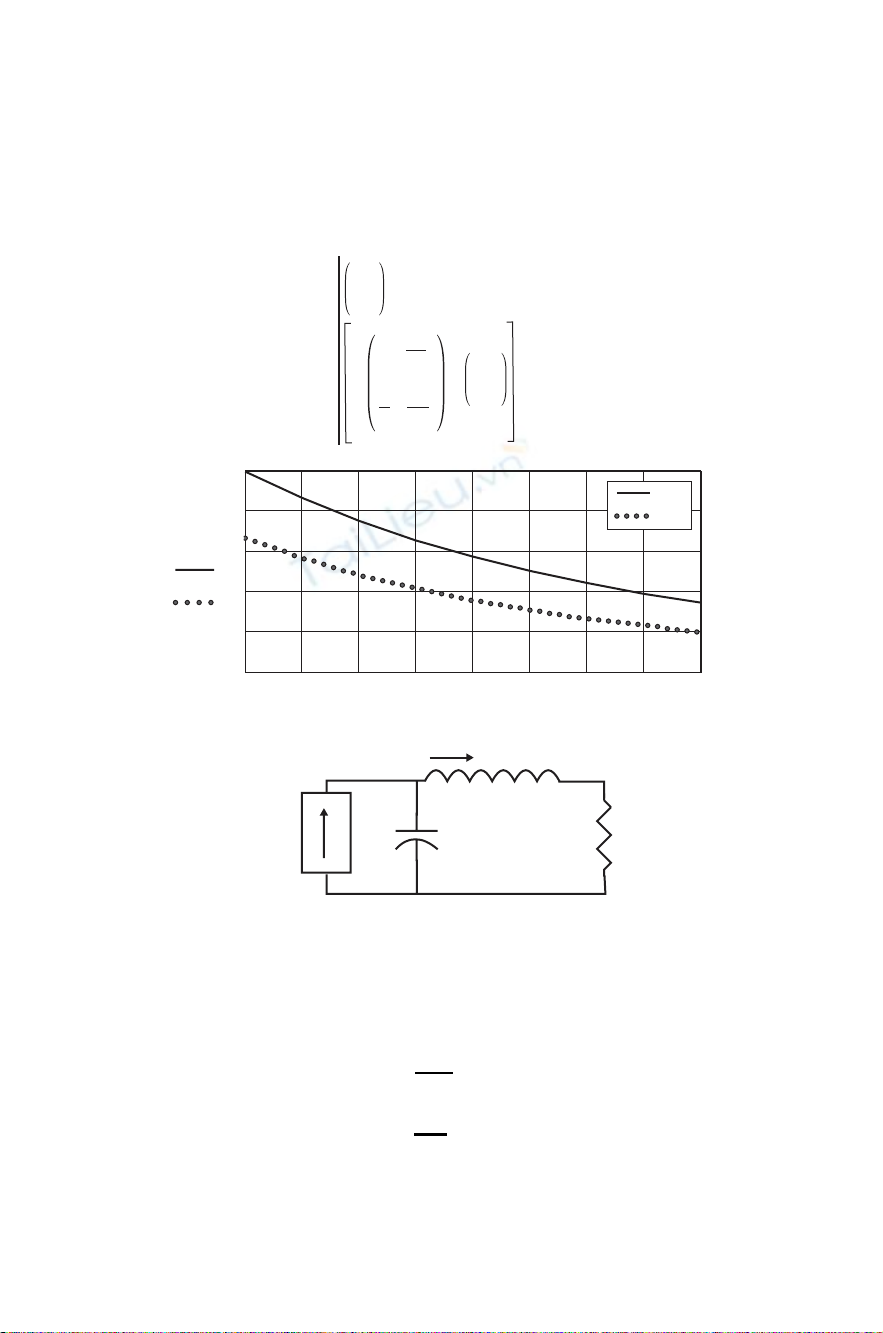
Solution to matrix differential equation for initial conditions of VC = 1.5, IL = 1.
0
C
L
R
IL
VC
VL
+
++
−
−
−
u(t) VOUT
T := 0.1
Figure A-2 LCR Circuit differential equation solution for initial values
of VCand IL,Igen =0.
iC=CdvC
dt =u−iL
vL=LdiL
dt =vC−RiL(A-3)
vOUT =RiL

ADDITIONAL DISCRETE-SIGNAL ANALYSIS AND DESIGN INFORMATION 157
Rewrite Eq. (A-3) in state-variable format:
v·
C=0vC−1
CiL+1
Cu
õ·
L=1
LvC−R
LiL+0u(A-4)
vO=RiL
A nodal circuit analysis conÞrms these facts for this example. R,L,
and Care constant values, but they can easily be time-varying and/or
nonlinear functions of voltage and current. The discrete analysis method
deals with all of this very nicely.
We now add in the initial conditions at time zero, VC0and IL0:
v·
C=0(vC+VC0)−1
C(iL+IL0)+1
Cu
õ·
L=1
L(vC+VC0)−R
L(iL+IL0)+0u(A-5)
vO=RiL
The two derivatives appear on the left side. Note that if (vC+VC0)is
multiplied by zero, the rate of change of vCdoes not depend on that term,
and the rate of change of iLdoes not depend on uif the uis multiplied
by zero. The options of Eqs. (A-4) and (A-5) can easily be imagined.
Description of ßow-graph methods in [Dorf and Bishop, 2004, Chaps.
2 and 3] and in numerous other references are excellent tools that are
commonly used for these problems. We will not be able to get deeply
into that subject in this book, but Fig. A-4 is an example.
The next step is to rewrite Eq. (A-5) in matrix format. Also, vCis now
called X1,andILis now called X2.
˙
X1
˙
X2=0−1
C
1
L−R
LX1
X2+1
C
0(u) (A-6)
VO=RX2

158 DISCRETE-SIGNAL ANALYSIS AND DESIGN
Now write the (A-6) equations as follows:
˙
X1=0X1−1
CX2+1
Cu
˙
X2=1
LX1−R
LX2+0u(A-7)
VO=RX2
Next, we will solve Eq. (A-6) [same as Eq. (A-7) for X1(=vc), X2
(=iL), and VO]. Component uis the input signal generator.
This general idea applies to a wide variety of practical problems (see
[Dorf and Bishop, 2004, Chap. 3] and many other references). The meth-
ods of matrix algebra and matrix calculus operations are found in many
handbooks (e.g., [Zwillinger, 1996]).
The general format for state-variable equations, similar to Eqs. (A-4)
and (A-5), is
˙
x=Ax +Bu
y=Cx +Du (A-8)
in which A, B, C,andDare coefÞcient matrices whose numbers may
be complex and varying in some manner with time, voltage, or current,
upertains to complex signal sources, and yis the complex output for a
complex input signal u. The boldface letters denote matrices speciÞcally.
Comparing Eq. (A-6) with Eq. (A-5), the general idea is clear. At any
time t,xis the collection (vector) of voltages vand currents iin the
circuit, and ˙
xis the collection (vector) of their time derivatives.
Matrix algebra or matrix calculus, using Mathcad, Þnds all the values
of xand yat each value of time twith great rapidity, and plots graphs
of the results. Starting at t= 0, from a set of initial values of Vand I,we
can trace the history of the network through the transient period and into
the steady state.
We will look more closely at the general method of matrix construc-
tion for our speciÞc example. Equations (A-6), (A-7), and (A-9) can be
Laplace-transformed. In this process the unit matrix [I]=10
01
,and
this work must be in accordance with the rules of matrix algebra and the

ADDITIONAL DISCRETE-SIGNAL ANALYSIS AND DESIGN INFORMATION 159
Laplace transform:
1.sX(s)−x(0)=AX(s) +BU(s)
2.sX(s)−AX(s) =x(0)+BU(s)
3.X(s)[sI −A]=x(0)+BU(s)
4.X(s)=[sI −A]−1x(0)+[sI −A]−1BU(s)
(A-9)
This can be inverse-Laplace-transformed to get x(t), a function of time
for each X(s) [Dorf and Bishop, 2004, Sec. 3], but we want to use the dis-
crete derivative of Eq. (A-2) as an alternative for discrete-signal analysis
and design [Dorf and Bishop, 2004, Sec. 3].
USING THE DISCRETE DERIVATIVE
We now replace the ˙xmatrix in Eq. (A-6) by incorporating Eq. (A-2).
Using the intermediate steps in Eq. (A-10) and using the sequence index
x(n) method that we are already very familiar with produces the following
Mathcad program, expressed in Word for Windows format.
1.(if n=0)x0(n)
x1(n)=VC0
IL0
2.(if n>0)x0(n)
x1(n)=T0−1
C
1
L−R
L+10
01
(A-10)
×x0(n−1)
x1(n−1)+Tb0
b1u(n)
Figure A-3 shows this equation in Mathcad program form. We can imme-
diately use three options:
1. Initial conditions x0(0) and x1(0) can be zero, u(n) can have a dc
value or a time function such as a step or sine wave, and in this
example [Eqs. (A-6) and (A-7)] b0=1, b1=0, T=0.1, u(n)=1.0.
2. u(n) can be zero, and the transient response is driven by x(0), an
initial value of capacitor voltage or inductor current or both.
160 DISCRETE-SIGNAL ANALYSIS AND DESIGN
N
:= 1000 n := 0,1.. N
b := u(n) := 100 sin
x(n) : = if n = 0
T+
0
1
L
−1
C
R
L
1
0
0
1
.x(n− 1) + T b u(n) if n > 0
T := 0.01 R := 0.01 L := 0.5 C := 0.5
1
0
2π 4mA
n
N
0
0
0 200 400 600 800 1000
−400
−200
0
200
400
V(C)
I(L)
n
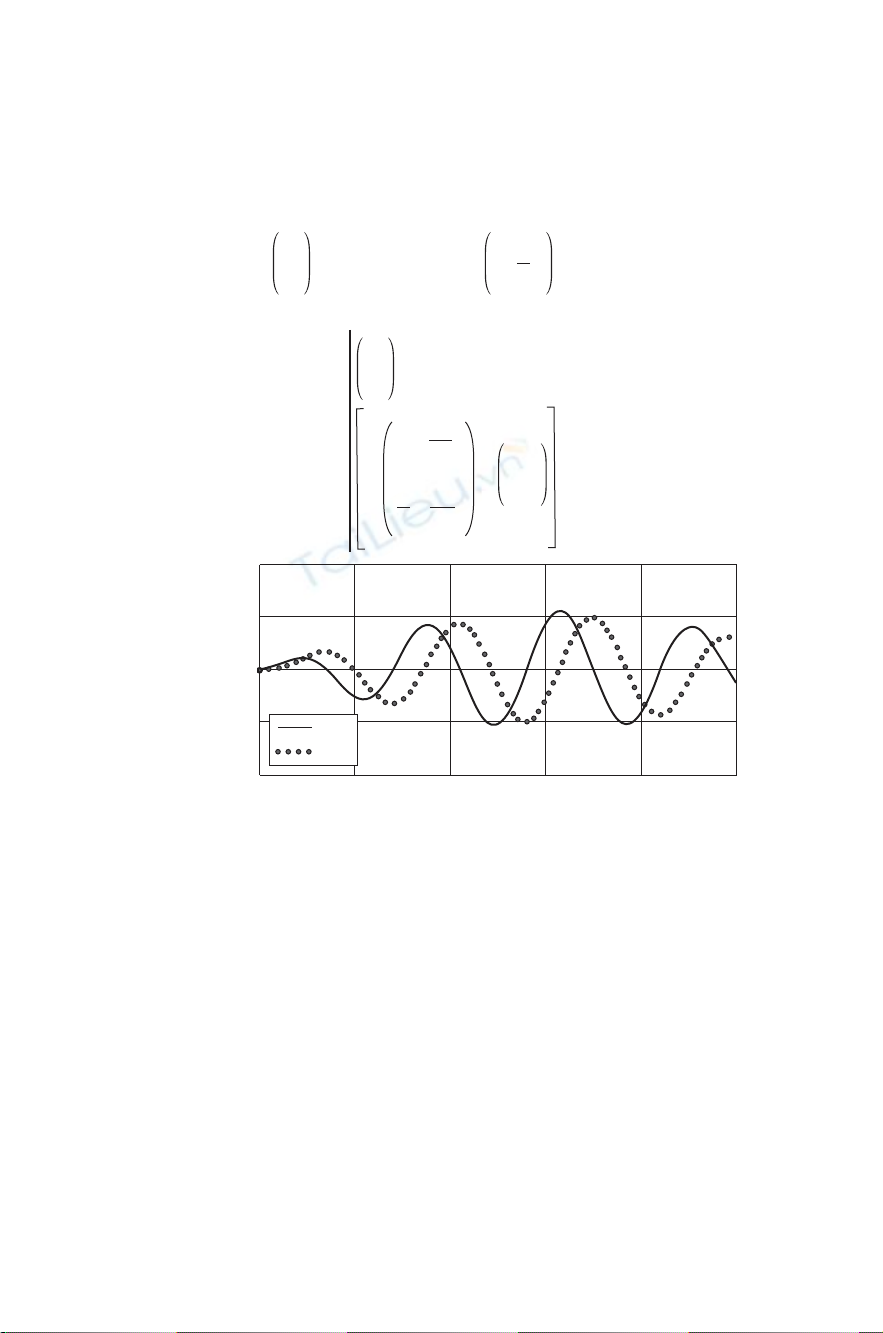
Figure A-3 Time response of the LCR network with zero initial condi-
tions and sine-wave current excitation.
3. x(0) and u(n) can both be operational at t=0 or later than zero.
There are a lot of options for this problem.
The Mathcad worksheet Fig. A-2 shows option 2 for initial condition
values of VCand IL,andu(n)=0. The values of x(n)0and x(n)1are
plotted.
Figure A-3 uses zero initial conditions and u(n)=100 mA sine wave,
frequency =4, b0=1.0, b1=0. The buildups from zero of x1(capacitor
volts) and x2(inductor amperes) are plotted. The lag of IL(peaks at a
later time) can be noticed.


![Ngân hàng đề thi trắc nghiệm Kiến trúc máy tính [mới nhất]](https://cdn.tailieu.vn/images/document/thumbnail/2026/20260514/hoahongxanh0906/135x160/49281779160279.jpg)


%20--%3e%3cdefs%3e%3cstyle%3e%20.st0%20{%20fill:%20%23fff;%20}%20.st1%20{%20fill:%20%237800fa;%20}%20%3c/style%3e%3c/defs%3e%3cpath%20class='st1'%20d='M117.78,12.18H43.11c2.9,3.47,4.65,7.94,4.65,12.82,0,5.6-2.3,10.66-6.01,14.29h76.02l7.22-13.56-7.22-13.56Z'/%3e%3cg%3e%3cpath%20class='st0'%20d='M53.58,26.17h-.59v-1.46h.59v-4.96h2.83c1.78,0,2.67.94,2.67,2.82v5.76c0,1.87-.89,2.81-2.67,2.81h-2.83v-4.96ZM55.36,21.37v3.34h1.1v1.46h-1.1v3.34h1.01c.61,0,.91-.37.91-1.1v-5.93c0-.74-.3-1.1-.91-1.1h-1.01Z'/%3e%3cpath%20class='st0'%20d='M65.99,31.14h-1.8l-.31-2.07h-2.19l-.31,2.07h-1.64l1.82-11.39h2.62l1.82,11.39ZM65.28,18.04c-.25.46-.51.77-.75.94-.21.15-.47.22-.79.22-.26,0-.57-.07-.92-.22l-.38-.15c-.14-.05-.26-.07-.37-.07-.3,0-.53.18-.71.54l-.91-.68c.25-.46.51-.77.75-.94.21-.14.48-.21.79-.21.26,0,.57.07.92.21l.38.15c.14.05.26.07.37.07.3,0,.53-.18.71-.54l.91.68ZM61.91,27.52h1.73l-.87-5.76-.87,5.76Z'/%3e%3cpath%20class='st0'%20d='M74.53,26.89v1.52c0,1.91-.89,2.86-2.67,2.86s-2.67-.95-2.67-2.86v-5.93c0-1.91.89-2.86,2.67-2.86s2.67.95,2.67,2.86v1.11h-1.69v-1.22c0-.75-.31-1.12-.93-1.12s-.93.37-.93,1.12v6.15c0,.74.31,1.11.93,1.11s.93-.37.93-1.11v-1.63h1.69Z'/%3e%3cpath%20class='st0'%20d='M81.4,31.14h-1.8l-.31-2.07h-2.19l-.31,2.07h-1.64l1.82-11.39h2.62l1.82,11.39ZM75.9,19.2l1.52-1.91h1.71l1.51,1.91h-1.61l-.76-.95-.75.95h-1.61ZM77.32,27.52h1.73l-.87-5.76-.87,5.76ZM83.1,15.99l-1.76,1.91h-1.26l1.17-1.91h1.86Z'/%3e%3cpath%20class='st0'%20d='M84.86,19.75c1.78,0,2.67.94,2.67,2.82v1.48c0,1.87-.89,2.81-2.67,2.81h-.85v4.28h-1.79v-11.39h2.64ZM84.01,21.37v3.86h.85c.58,0,.87-.36.87-1.08v-1.71c0-.71-.29-1.07-.87-1.07h-.85Z'/%3e%3cpath%20class='st0'%20d='M93.51,19.75c1.78,0,2.67.94,2.67,2.82v1.48c0,1.87-.89,2.81-2.67,2.81h-.85v4.28h-1.79v-11.39h2.64ZM92.66,21.37v3.86h.85c.58,0,.87-.36.87-1.08v-1.71c0-.71-.29-1.07-.87-1.07h-.85Z'/%3e%3cpath%20class='st0'%20d='M98.8,31.14h-1.79v-11.39h1.79v4.88h2.03v-4.88h1.83v11.39h-1.83v-4.88h-2.03v4.88Z'/%3e%3cpath%20class='st0'%20d='M105.36,24.55h2.46v1.62h-2.46v3.34h3.09v1.63h-4.88v-11.39h4.88v1.63h-3.09v3.18ZM108.17,17.29l-1.76,1.91h-1.26l1.17-1.91h1.86Z'/%3e%3cpath%20class='st0'%20d='M112.2,19.75c1.78,0,2.67.94,2.67,2.82v1.48c0,1.87-.89,2.81-2.67,2.81h-.85v4.28h-1.79v-11.39h2.64ZM111.35,21.37v3.86h.85c.58,0,.87-.36.87-1.08v-1.71c0-.71-.29-1.07-.87-1.07h-.85Z'/%3e%3c/g%3e%3ccircle%20class='st1'%20cx='25'%20cy='25'%20r='20'/%3e%3cpath%20class='st0'%20d='M32.78,19.27c2.92,0,4.43,2.55,5.28,5.33l.71,2.17c.14.38-.33.75-.71.75h-5.61c.19-.33.24-.71.09-1.08l-.75-2.45c-.43-1.32-.99-2.64-1.79-3.77.75-.57,1.65-.94,2.78-.94h0ZM25,18.38c3.25,0,4.9,2.78,5.89,5.89l.76,2.45c.14.42-.33.8-.8.8h-11.69c-.42,0-.94-.38-.8-.8l.75-2.45c.99-3.11,2.64-5.89,5.89-5.89h0ZM25,11.35c1.74,0,3.11,1.37,3.11,3.11s-1.37,3.11-3.11,3.11-3.11-1.41-3.11-3.11,1.41-3.11,3.11-3.11h0ZM17.27,19.27c1.08,0,1.98.38,2.73.94-.8,1.13-1.37,2.45-1.74,3.77l-.8,2.45c-.14.38-.05.75.09,1.08h-5.56c-.42,0-.9-.38-.75-.75l.71-2.17c.9-2.78,2.41-5.33,5.33-5.33h0ZM17.27,12.91c1.51,0,2.78,1.27,2.78,2.83s-1.27,2.83-2.78,2.83-2.83-1.27-2.83-2.83,1.27-2.83,2.83-2.83h0ZM32.78,12.91c1.56,0,2.78,1.27,2.78,2.83s-1.23,2.83-2.78,2.83-2.83-1.27-2.83-2.83,1.27-2.83,2.83-2.83h0ZM27.07,28.56v.09c0,.57-.24,1.08-.61,1.46h0v.05c-.38.33-.9.57-1.46.57s-1.08-.24-1.46-.61h0c-.38-.38-.61-.9-.61-1.46v-.09h1.41v.09c0,.19.05.38.19.47v.05c.09.09.28.19.47.19s.38-.09.47-.19v-.05c.14-.09.24-.28.24-.47t-.05-.09h1.41ZM30.99,28.56v.09c0,1.65-.66,3.16-1.74,4.24-1.08,1.08-2.59,1.79-4.24,1.79s-3.16-.71-4.24-1.79l-.05-.05c-1.04-1.08-1.7-2.55-1.7-4.2v-.09h1.41v.09c0,1.27.47,2.4,1.27,3.25h.05c.85.85,1.98,1.37,3.25,1.37s2.4-.52,3.25-1.37c.85-.8,1.37-1.98,1.37-3.25v-.09h1.37ZM34.99,28.56v.09c0,2.78-1.13,5.28-2.92,7.07-1.79,1.79-4.29,2.92-7.07,2.92s-5.23-1.13-7.07-2.92c-1.79-1.79-2.92-4.29-2.92-7.07v-.09h1.41v.09c0,2.4.94,4.53,2.5,6.08,1.56,1.56,3.72,2.5,6.08,2.5s4.52-.94,6.08-2.5c1.56-1.56,2.5-3.68,2.5-6.08v-.09h1.41Z'/%3e%3c/svg%3e)