Utilitarian Pricing of Annuities •111
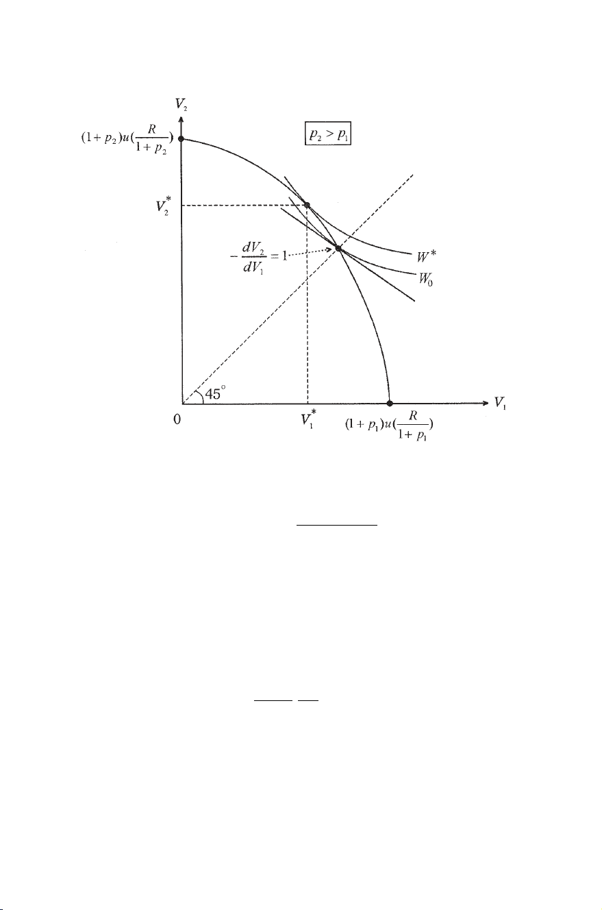
Figure 13.1. First-best allocation of utilities.
while
V∗
h=(1 +ph)uR
H
h=1(1 +ph).
Thus, the utilitarian first best has inequality in expected utilities but may
have equality in consumption levels (Arrow, 1992).
This result is similar to Mirrlees’ (1971) optimum income tax model
where individuals differ in productivity.2The first best allocation pro-
vides higher (expected) utility to those with a higher capacity to produce
utility.
In the appendix to this chapter it is shown that
0>1+pn
c∗
h
∂c∗
h
∂ph
>−1,(13.7)
while ∂c∗
h/∂pj0,for j= h,h,j=1,2,..., n.
2In Mirrlees’ model with additive utilities, the first best has all individuals with equal
consumption, and those with higher productivity, having a lower disutility for generating a
given income, are assigned to work more and hence have a lower utility.

112 •Chapter 13
Concavity of uand (13.7) imply
∂V∗
h
∂ph
=u(c∗
h)+(1 +pn)u′(cn)∂c∗
h
∂pn
>0,(13.8)
while ∂V∗
h/∂pj0,j= h,j=1,2,...,H.3Thus, with the given total
resources, an increase in one individual’s survival probability decreases
his or her optimum consumption, but the positive effect of higher survival
probability on expected utility dominates. The effect on the welfare
of other individuals facing only resource redistribution depends on the
shape of the social welfare function.
13.2Competitive Annuity Market with Full Information
In a competitive market with full information on the survival proba-
bilities of individuals and a zero rate of interest, the price of a unit of
second-period consumption, c2h, is equal to the survival probability of
each annuitant. Individuals maximize expected utility subject to a budget
constraint
c1h+phc2h=yhh=1,2,..., H,(13.9)
where yhis the given income of individual h. Demands for first- and
second-period consumption (annuities),
c1hand
c2h, are given by
c1h=
c2h=
ch=yh/(1 +ph).
The first-best allocation can be supported by a competitive annuity
market accompanied by an optimum income allocation. Equating con-
sumption levels under competition,
ch,to the optimum levels, c∗
h(p),
yields unique income levels,
yh=(1 +ph)c∗
h(p),that support the first-best
allocation. In particular, with an additive W, all individuals consume the
same amount:
c∗
h=R
H
h=1(1 +ph),
hence
yh=1+ph
H
h=1(1 +ph)R.(13.10)
3In the extreme case when W=min[V
1,V
2,...,VH], optimum expected utilities,
V∗
h=(1 +ph)u(c∗
h), are equal, and hence optimum consumption, c∗
h, strictly decreases
with ph(and increases with pj,j= h).

Utilitarian Pricing of Annuities •113
13.3Second-best Optimum Pricing of Annuities
Governments do not engage, for well-known reasons, in unconstrained
lump-sum redistributions of incomes. In contrast, most annuities
are supplied directly by government-run social security systems and
taxes/subsidies can, if so desired, be applied to the prices of annuities
offered by private pension funds. These prices can be used by govern-
ments to improve social welfare. Although deviations from actuarially
fair prices entail distortions (i.e., efficiency losses), distributional im-
provements may outweigh the costs.4
Suppose that individual hpurchases annuities at a price of qh.With
an income yh, his or her budget constraint is
c1h+qhc2h=yh,h=1,2...,H.(13.11)
Maximization of (13.2) subject to (13.11) yields demands
cih =
cih(qh,ph,yh), i=1,2,and h=1,2,...,H. Maximized expected utility,
V
h,is
V
h(qh,ph,yh)=u(
c1h)+phu(
c2h).
Assume that no outside resources are available for the annuity market,
hence total subsidies/taxes must equal zero,
H
h=1
(qh−ph)
c2h=0.(13.12)
Maximization of W(
V
1,
V
2,...,
VH) with respect to prices (q1,...,qH)
subject to (13.12) yields the first-order condition
∂W
∂
V
h
∂
V
h
∂qh
+λ
c2h+(qh−ph)∂
c2h
dqh=0,h=1,2,...,H,(13.13)
where λ>0 is the shadow price of constraint (13.12). In elasticity form,
using Roy’s identity (∂
V
h/∂qh=−(∂
V
h/∂yh)
c2h), (13.13) can be written
qh−ph
qh
=θh
εh
,(13.14)
where εh=−(qh/
c2h)(∂
c2h/dqh)istheprice elasticity of second-period
consumption of individual hand
θh=1−1
λ
∂W
∂
V
h
∂
V
h
∂yh
4In practice, of course, prices do not vary individually. Rather, individuals with similar
survival probabilities are grouped into risk classes, and annuity prices and taxes/subsidies
vary across these classes.

114 •Chapter 13
is the net social value of a marginal transfer to individual hthrough the
optimum pricing scheme. Equation (13.14) is a variant of the well-known
inverse elasticity optimum tax formula, which combines equity (θh) and
efficiency (1/εh) considerations.
The implication of (13.14) for the optimum pricing of annuities
depends on the welfare function, W, and on the joint distribution of
incomes, (y1,...,yH), and probabilities, (p1,..., pH).
To obtain some concrete examples, let Wbe the sum of expected
utilities. Then ∂W/∂
V
h=1,h=1,2,...,H. Assume further that
V
h=ln c1h+phln c2h. In this case, demands are
c1h=yh
1+ph
,
c2h=yh
1+ph
ph
qh
,(13.15)
and
V
h=(1+ph)ln yh
1+ph+phln ph
qh.(13.16)
Conditions (13.14) and (13.12) now yield the solution
qh=φβh
H
h=1βh,(13.17)
where
φ=
H
h=1
ph>0 and βh=phyh
1+ph
>0.
Consider two special cases of (13.17):
(a) Equal incomes: (yh=y=R/H;h=1,2,...,H)
Condition (13.17) now becomes qh=¯
φ(ph/(1 +ph)),where
¯
φ=H
h=1ph
H
h=1ph
1+ph(>1).(13.18)
It is seen (figure 13.2) that optimum pricing involves subsidization
(taxation) of individuals with high (low) survival probabilities.5
5In figure 13.2, it can be shown that ¯
φ/2<1.
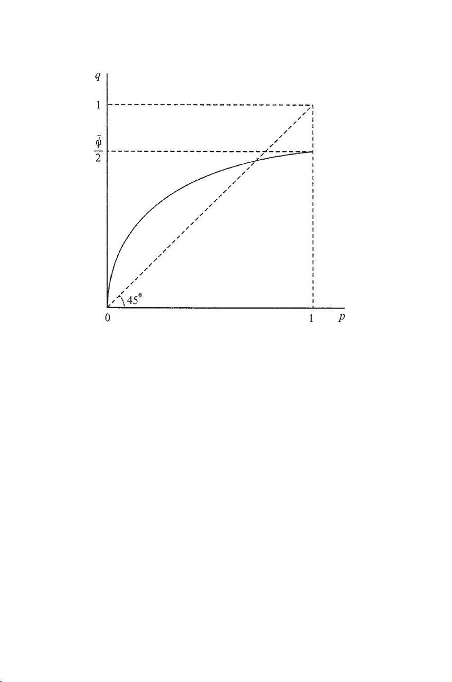
Utilitarian Pricing of Annuities •115
Figure 13.2. Optimum annuity pricing in a full-information equilibrium.
(b) yh=y(1 +ph)
This, one recalls, is the first-best utilitarian income distribution, and since
all price elasticities are equal to unity, we see from (13.17), as expected,
that qh=ph; that is efficiency prices are optimal.
More generally, it is seen from (13.17) that a higher correlation
between incomes, yh, and survival probabilities, ph, decreases—and
possibly eliminates—the subsidization of high-survival individuals.
In contrast, a negative correlation between incomes and survival
probabilities (as, presumably, in the female/male case) leads to subsidies
for high- survival individuals, possibly to the commonly observed
uniform pricing rule.


![Tín dụng trung-dài hạn: Những vấn đề cơ bản [chuẩn nhất]](https://cdn.tailieu.vn/images/document/thumbnail/2013/20131120/butmauden/135x160/6441384999291.jpg)


![Đề thi giữa học kì Tài chính tiền tệ: Tổng hợp [Năm]](https://cdn.tailieu.vn/images/document/thumbnail/2026/20260513/hoacattuong2026/135x160/81291778835177.jpg)


![320 câu hỏi trắc nghiệm Nghiệp vụ Ngân hàng có đáp án [Mới nhất]](https://cdn.tailieu.vn/images/document/thumbnail/2026/20260407/zinedinezidane06/135x160/49541776134685.jpg)

%20--%3e%3cdefs%3e%3cstyle%3e%20.st0%20{%20fill:%20%23fff;%20}%20.st1%20{%20fill:%20%237800fa;%20}%20%3c/style%3e%3c/defs%3e%3cpath%20class='st1'%20d='M117.78,12.18H43.11c2.9,3.47,4.65,7.94,4.65,12.82,0,5.6-2.3,10.66-6.01,14.29h76.02l7.22-13.56-7.22-13.56Z'/%3e%3cg%3e%3cpath%20class='st0'%20d='M53.58,26.17h-.59v-1.46h.59v-4.96h2.83c1.78,0,2.67.94,2.67,2.82v5.76c0,1.87-.89,2.81-2.67,2.81h-2.83v-4.96ZM55.36,21.37v3.34h1.1v1.46h-1.1v3.34h1.01c.61,0,.91-.37.91-1.1v-5.93c0-.74-.3-1.1-.91-1.1h-1.01Z'/%3e%3cpath%20class='st0'%20d='M65.99,31.14h-1.8l-.31-2.07h-2.19l-.31,2.07h-1.64l1.82-11.39h2.62l1.82,11.39ZM65.28,18.04c-.25.46-.51.77-.75.94-.21.15-.47.22-.79.22-.26,0-.57-.07-.92-.22l-.38-.15c-.14-.05-.26-.07-.37-.07-.3,0-.53.18-.71.54l-.91-.68c.25-.46.51-.77.75-.94.21-.14.48-.21.79-.21.26,0,.57.07.92.21l.38.15c.14.05.26.07.37.07.3,0,.53-.18.71-.54l.91.68ZM61.91,27.52h1.73l-.87-5.76-.87,5.76Z'/%3e%3cpath%20class='st0'%20d='M74.53,26.89v1.52c0,1.91-.89,2.86-2.67,2.86s-2.67-.95-2.67-2.86v-5.93c0-1.91.89-2.86,2.67-2.86s2.67.95,2.67,2.86v1.11h-1.69v-1.22c0-.75-.31-1.12-.93-1.12s-.93.37-.93,1.12v6.15c0,.74.31,1.11.93,1.11s.93-.37.93-1.11v-1.63h1.69Z'/%3e%3cpath%20class='st0'%20d='M81.4,31.14h-1.8l-.31-2.07h-2.19l-.31,2.07h-1.64l1.82-11.39h2.62l1.82,11.39ZM75.9,19.2l1.52-1.91h1.71l1.51,1.91h-1.61l-.76-.95-.75.95h-1.61ZM77.32,27.52h1.73l-.87-5.76-.87,5.76ZM83.1,15.99l-1.76,1.91h-1.26l1.17-1.91h1.86Z'/%3e%3cpath%20class='st0'%20d='M84.86,19.75c1.78,0,2.67.94,2.67,2.82v1.48c0,1.87-.89,2.81-2.67,2.81h-.85v4.28h-1.79v-11.39h2.64ZM84.01,21.37v3.86h.85c.58,0,.87-.36.87-1.08v-1.71c0-.71-.29-1.07-.87-1.07h-.85Z'/%3e%3cpath%20class='st0'%20d='M93.51,19.75c1.78,0,2.67.94,2.67,2.82v1.48c0,1.87-.89,2.81-2.67,2.81h-.85v4.28h-1.79v-11.39h2.64ZM92.66,21.37v3.86h.85c.58,0,.87-.36.87-1.08v-1.71c0-.71-.29-1.07-.87-1.07h-.85Z'/%3e%3cpath%20class='st0'%20d='M98.8,31.14h-1.79v-11.39h1.79v4.88h2.03v-4.88h1.83v11.39h-1.83v-4.88h-2.03v4.88Z'/%3e%3cpath%20class='st0'%20d='M105.36,24.55h2.46v1.62h-2.46v3.34h3.09v1.63h-4.88v-11.39h4.88v1.63h-3.09v3.18ZM108.17,17.29l-1.76,1.91h-1.26l1.17-1.91h1.86Z'/%3e%3cpath%20class='st0'%20d='M112.2,19.75c1.78,0,2.67.94,2.67,2.82v1.48c0,1.87-.89,2.81-2.67,2.81h-.85v4.28h-1.79v-11.39h2.64ZM111.35,21.37v3.86h.85c.58,0,.87-.36.87-1.08v-1.71c0-.71-.29-1.07-.87-1.07h-.85Z'/%3e%3c/g%3e%3ccircle%20class='st1'%20cx='25'%20cy='25'%20r='20'/%3e%3cpath%20class='st0'%20d='M32.78,19.27c2.92,0,4.43,2.55,5.28,5.33l.71,2.17c.14.38-.33.75-.71.75h-5.61c.19-.33.24-.71.09-1.08l-.75-2.45c-.43-1.32-.99-2.64-1.79-3.77.75-.57,1.65-.94,2.78-.94h0ZM25,18.38c3.25,0,4.9,2.78,5.89,5.89l.76,2.45c.14.42-.33.8-.8.8h-11.69c-.42,0-.94-.38-.8-.8l.75-2.45c.99-3.11,2.64-5.89,5.89-5.89h0ZM25,11.35c1.74,0,3.11,1.37,3.11,3.11s-1.37,3.11-3.11,3.11-3.11-1.41-3.11-3.11,1.41-3.11,3.11-3.11h0ZM17.27,19.27c1.08,0,1.98.38,2.73.94-.8,1.13-1.37,2.45-1.74,3.77l-.8,2.45c-.14.38-.05.75.09,1.08h-5.56c-.42,0-.9-.38-.75-.75l.71-2.17c.9-2.78,2.41-5.33,5.33-5.33h0ZM17.27,12.91c1.51,0,2.78,1.27,2.78,2.83s-1.27,2.83-2.78,2.83-2.83-1.27-2.83-2.83,1.27-2.83,2.83-2.83h0ZM32.78,12.91c1.56,0,2.78,1.27,2.78,2.83s-1.23,2.83-2.78,2.83-2.83-1.27-2.83-2.83,1.27-2.83,2.83-2.83h0ZM27.07,28.56v.09c0,.57-.24,1.08-.61,1.46h0v.05c-.38.33-.9.57-1.46.57s-1.08-.24-1.46-.61h0c-.38-.38-.61-.9-.61-1.46v-.09h1.41v.09c0,.19.05.38.19.47v.05c.09.09.28.19.47.19s.38-.09.47-.19v-.05c.14-.09.24-.28.24-.47t-.05-.09h1.41ZM30.99,28.56v.09c0,1.65-.66,3.16-1.74,4.24-1.08,1.08-2.59,1.79-4.24,1.79s-3.16-.71-4.24-1.79l-.05-.05c-1.04-1.08-1.7-2.55-1.7-4.2v-.09h1.41v.09c0,1.27.47,2.4,1.27,3.25h.05c.85.85,1.98,1.37,3.25,1.37s2.4-.52,3.25-1.37c.85-.8,1.37-1.98,1.37-3.25v-.09h1.37ZM34.99,28.56v.09c0,2.78-1.13,5.28-2.92,7.07-1.79,1.79-4.29,2.92-7.07,2.92s-5.23-1.13-7.07-2.92c-1.79-1.79-2.92-4.29-2.92-7.07v-.09h1.41v.09c0,2.4.94,4.53,2.5,6.08,1.56,1.56,3.72,2.5,6.08,2.5s4.52-.94,6.08-2.5c1.56-1.56,2.5-3.68,2.5-6.08v-.09h1.41Z'/%3e%3c/svg%3e)