
185
Array Beamforming
separation dwavelengths, by a pseudorandom step chosen within an interval
of width d−0.5, which ensures that the elements are at least half a wavelength
apart. Figure 7.10(a) shows the response in uspace for an array of 21 elements
at an average spacing of 2/3. A sector beam of width 40 degrees centered at
broadside was specified. A regular array would have a pattern repetitive at
an interval of 1.5 in u, and this is shown by the dotted response. The
irregular array ‘‘repetitions’’ are seen to degrade rapidly, but the pattern that
matters is that lying in the interval [−1, 1] in u. This part of the response
leads to the actual pattern in real space, shown in Figure 7.10(b). We note
that the side lobes are up to about −13 dB, rather poorer than for the
patterns from regular arrays shown in Figures 7.6, 7.8, and 7.9, though this
level varies considerably with the actual set of element positions chosen. The
integration interval I was chosen to be [−1, 1], to give the least squared
error solution over the full angle range (from −90 degrees to +90 degrees,
and its reflection about the line of the array).
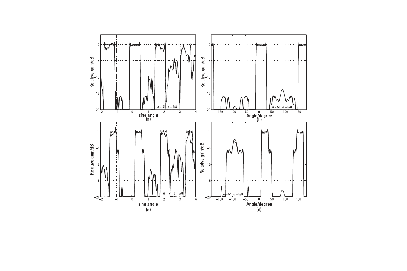
A second example is given in Figure 7.11 for an array of 51 elements,
but illustrating the effect of steering. In Figure 7.11(a, b) the 40-degree
beam is steered to 10 degrees, and again we see the rapid deterioration of
the approximate repetitions in uspace of the beam, and a nonsymmetric
side-lobe pattern, though the levels are roughly comparable with those of
the first array. The average separation is 0.625 wavelengths, giving a repetition
interval of 1.6 in u. If we steer the beam to 30 degrees [Figure 7.10(c, d)],
there is a marked deterioration in the beam quality. This is because one of
the repetitions falls within the interval I over which the pattern error is
minimized, so the part of this beam (near u=−1) that should be zero is
reduced. At the same time the corresponding part of the wanted beam (near
u=
1
⁄
2
) should be unity, so the solution tries to hold this level up. We note
that the levels end up close to −6 dB, which corresponds to an amplitude
of 0.5, showing that the error has been equalized between these two require-
ments. We note from the dotted responses that the result would be much
the same using a regular array. In fact, this problem would be avoided by
choosing I to be of width 1.6 (the repetition interval) instead of 2, preserving
the quality of the sector beam, but in this case the large lobe around −90
degrees would be the full height, near 0 dB. Even if this solution (with a
large grating lobe) were acceptable for the regular array, it is not so satisfactory
for the irregular array as the distorted repetitions start to spread into the
basic least squares estimation interval, as the array becomes more irregular,
creating more large side lobes.
Thus, although a solution can be found for the irregular array, its
usefulness is limited for two reasons; the set of nonorthogonal exponential
186 Fourier Transforms in Radar and Signal Processing
Figure 7.11 Sector patterns from a steered irregular linear array: (a) response in u-space, beam at 10 degrees; (b) beam pattern, beam at
10°; (c) response in u-space, beam at 30°; (d) beam pattern, beam at 30°.

187
Array Beamforming
functions (from the irregular array positions) used to form the required
pattern is not as good as the set used in the regular case, and if the element
separation is to be 0.5 wavelength as a minimum, an irregular array must
have a mean separation of more than 0.5 wavelength, leading to grating (or
approximate grating) effects.
7.5 Summary
As there is a Fourier transform relationship between the current excitation
across a linear aperture and the resultant beam pattern (in terms of u,a
direction cosine coordinate), there is the opportunity to apply the rules-and-
pairs methods for suitable problems in beam pattern design. This has the
now familiar advantage of providing clarity in the relationship between
aperture distribution and beam patterns, where both are expressed in terms
of combinations of relatively simple functions.
However, there is the complication to be taken into account that the
‘‘angle’’ coordinate in this case is not the physical angle but the direction
cosine along the line of the aperture. In the text we have taken the angle
u
to be measured from broadside to the aperture, and defined the corresponding
Fourier transform variable uas sin
u
, so that u=cos (
p
/2 −
u
), the cosine
of the angle measured from the line along the aperture. In this udomain,
beam shapes remain constant as beams are steered, while in real space
they become stretched out when steered towards the axis of the aperture.
Furthermore, the transform of the aperture distribution produces a function
that can be evaluated for all real values of u, but only the values of ulying
in the range −1 to 1 correspond to real directions.
Both continuous apertures and discrete apertures can be analyzed, the
latter corresponding to ideal antenna arrays, with point, omnidirectional,
elements. In this chapter we have concentrated on the discrete, or array,
case. The regular linear array, which is very commonly encountered, is
particularly amenable to the rules-and-pairs form of analysis. In this case,
the regular distribution (a comb function) produces a periodic pattern in u
space (a rep function). In the case of a directional beam, the repetitions of
this beam are potential grating lobes, which are generally undesirable, but
if the repetition interval is adequate, there will be no repetitions within the
basic interval in ucorresponding to real space and hence no grating lobes.
The condition for this (that the elements be no more than half a wavelength
apart) is very easily found by this approach. Two variations on the directional
beam for producing different low side-lobe patterns were studied in Section

188 Fourier Transforms in Radar and Signal Processing
7.3.1. These exercises, whether or not leading to useful solutions for practical
application, are intended to illustrate how the rules-and-pairs methods can
be applied to achieve solutions to relatively challenging problems with quite
modest effort. It was seen in Section 7.3.3 that very good beams covering
a sector at constant gain can be produced, again very easily, using the rules-
and-pairs method.
The case of irregular linear arrays can also be tackled by these methods.
However, the rules-and-pairs technique is not appropriate for finding directly
the discrete aperture distribution that will give a specified pattern when the
elements are irregularly placed. Instead, the problem is formulated as a least
squared error match between the pattern generated by the array and the
required one. In this case, the discrete aperture distribution is found to be
the solution of a set of linear equations, conveniently expressed in vector-
matrix form. The elements of both the vector and the matrix are obtained
as Fourier transform functions evaluated at points defined by the array
element positions. Again the sector pattern problem was taken and it was
shown that this approach gives the same solution as that given directly by
the Fourier transform in the case of the regular array, confirming that this
solution is indeed the least squared error solution. For the irregular array,
we obtain sector patterns as required, though with perhaps higher side-lobe
levels and with some limitations on the array (not too irregular or too wide
an aperture) and on the angle to which the beam can be steered away
from broadside. These limitations are not weaknesses of the method, but a
consequence of the irregular array structure that makes achieving a given
result more difficult.

Final Remarks
The illustrations of the use of the rules and pairs technique in Chapters 3
to 7 show a wide range of applications and how some quite complex problems
can be tackled using a surprisingly small set of Fourier transform pairs. The
method seems to be very successful, but on closer inspection we note that
the functions handled are primarily amplitude functions—the only phase
function is the linear phase function due to delay. Topics such as the spectra
of chirp (linear frequency modulated) pulses or nonlinear phase equalization
have not been treated, as the method, at least as at present formulated, does
not handle these. There may be an opportunity here to develop a similar
calculus for these cases.
A considerable amount of work, in Chapters 5 and 6, is directed at
showing the benefits of oversampling (only by a relatively small factor in
some cases) in reducing the amount of computation needed in the signal
processing under consideration. As computing speed is increasing all the time,
it is sometimes felt that little effort should go into reducing computational
requirements. However, apart from the satisfaction of achieving a more
elegant solution to a problem, there may be good practical reasons. Rather
analogously to C. Northcote Parkinson’s law, ‘‘work expands so as to fill
the time available for its completion,’’ there seems to be a technological
equivalent: ‘‘user demands rise to meet (or exceed) the capabilities of equip-
ment.’’ While at any time an advance in speed of computation may enable
current problems to be handled comfortably, allowing the use of inefficient
implementations, requirements will soon rise to take advantage of the
increased performance—for example, higher bandwidth systems, more real-
189
![Tập bài giảng Xử lý tín hiệu số [chuẩn nhất]](https://cdn.tailieu.vn/images/document/thumbnail/2021/20211119/cucngoainhan3/135x160/1203186432.jpg)


![Câu hỏi trắc nghiệm Lập trình C [mới nhất]](https://cdn.tailieu.vn/images/document/thumbnail/2025/20251012/quangle7706@gmail.com/135x160/91191760326106.jpg)