Journal of Cleaner Production 448 (2024) 141424
Available online 23 February 2024
0959-6526/© 2024 Elsevier Ltd. All rights reserved.
Review
Greenhouse gas accounting methodologies for wastewater treatment plants:
A review
Lailai Huang
a
,
b
, Hanxiang Li
a
,
b
,
**
, Yong Li
a
,
b
,
*
a
School of Environmental Science and Engineering, Suzhou University of Science and Technology, Suzhou, 215009, PR China
b
Jiangsu Provincial Key Laboratory of Environmental Science and Engineering, Suzhou University of Science and Technology, Suzhou, 215009, PR China
ARTICLE INFO
Handling editor: Jing Meng
Keywords:
Wastewater treatment
Greenhouse gas emissions
Emission factor method
Field monitoring method
Modeling method
ABSTRACT
Greenhouse gas (GHG) emissions from wastewater treatment plants (WWTPs) have become a major concern in
the efforts to mitigate climate change and reduce overall emissions. Carbon emission accounting methods are
direct strategies for obtaining carbon emission data from wastewater plants, but different accounting methods
have certain limitations. In this study, the development history, the scope of application, the advantages and
disadvantages of the emission factor, field monitoring, modeling methods, and machine learning methods were
discussed. The reliability and accuracy of different accounting methods for direct and indirect emissions were
compared and analyzed. In addition, the application progress of the accounting methods in developed and
developing countries was discussed. This study shows that the specificity of emission factors directly affects the
results obtained using the emission factor method. The field monitoring method is a relatively accurate approach,
but it relies on new technology and a monitoring cycle of more than one year. The results obtained from long-
term monitoring of the Anaerobic Oxic (AO) process are statistically greater (nitrous oxide (N
2
O) emissions
averaging 2.25% of the nitrogen loading) than those obtained from short-term monitoring (N
2
O emissions
averaging 0.032% of the nitrogen loading). The accuracy of the modeling approach relies on a good under-
standing of the pollutant fractions in the influent and the pollutant transformation mechanisms. In developed
countries, compared to developing countries, most of the studies were conducted using on-site monitoring and
modeling methods. In China, the emission factor method is used, which accounts for 44.4% of the total number of
publications. Future research could refine the various GHG calculation methods and improve the accuracy of the
calculations to meet the accounting needs of different wastewater treatment processes and different research
objectives. This study provides insight into developing low carbon wastewater treatment processes and routes. It
will also provide a reference for WWTPs to achieve carbon emission reduction.
1. Introduction
Global warming has increased the frequency and intensity of extreme
weather and natural disaster events. The global climate change tipping
point indicates that if not controlled, climate change is expected to cost
the global economy $178 trillion over the next 50 years (CPA Canada,
2023). In 2023, the Intergovernmental Panel on Climate Change (IPCC)
pointed out that greenhouse gas (GHG) emissions from human activities
contributed to global warming. Between 2011 and 2020, the global
surface temperature rose by 1.1 ◦C over 1850–1900 due to greenhouse
gas emissions. In addition, the report highlights the need for consider-
able, rapid, and sustained efforts to reduce GHG emissions across all
sectors (IPCC, 2023). Accurate accounting of GHG emissions is a top
priority when developing a GHG reduction strategy.
According to the United Nations, the global carbon emissions of
water treatment industries, such as wastewater treatment, account for
approximately 2% of global carbon emissions (Delanka-Pedige et al.,
2021). Rennert et al. (2022) have estimated that a metric tonne of car-
bon dioxide causes $185 worth of harm to society, taking into account
factors like energy, agriculture, sea levels, and mortality rates. Accord-
ing to recent estimates, the yearly emissions of greenhouse gases from
wastewater treatment facilities worldwide amount to around 1.43
billion metric tonnes, with a corresponding social cost of $264.5 billion
(X. He et al., 2023). Furthermore, Qadir et al. (2020) forecast a global
* Corresponding author. School of Environmental Science and Engineering, Suzhou University of Science and Technology, Suzhou, 215009, PR China.
** Corresponding author. School of Environmental Science and Engineering, Suzhou University of Science and Technology, Suzhou, 215009, PR China.
E-mail addresses: hanxiang_li@usts.edu.cn (H. Li), yongli69@163.com (Y. Li).
Contents lists available at ScienceDirect
Journal of Cleaner Production
journal homepage: www.elsevier.com/locate/jclepro
https://doi.org/10.1016/j.jclepro.2024.141424
Received 19 June 2023; Received in revised form 3 February 2024; Accepted 22 February 2024

Journal of Cleaner Production 448 (2024) 141424
2
increase in wastewater production by 24% by 2030 and 51% by 2050.
According to the International Energy Agency (IEA) 2018 report, if cities
around the world follow the modern typical technology blueprint for
centralised wastewater capacity, electricity consumption could increase
by over 680 TWh over the period to 2030. This increased demand for
electricity signifies a rise in energy production, particularly if the ma-
jority of this energy is derived from fossil fuels such as coal or natural
gas, leading to an increase in GHG emissions. Therefore, despite
wastewater treatment plants (WWTPs) substantially benefit urban en-
vironments, they continuously face challenges in terms of energy con-
sumption and GHG emissions. Controlling GHG emissions from
wastewater treatment facilities is therefore crucial.
The wastewater treatment process directly and indirectly emits GHG.
Methane (CH
4
) and nitrous oxide (N
2
O) are GHG that are produced and
directly emitted during wastewater and sludge treatment. The discharge
of CH
4
occurs in large quantities in wastewater transmission pipelines
and anaerobic treatment processes (Guisasola et al., 2008). N
2
O is
associated with the biological nitrogen transformation processes (Solis
et al., 2022). Massara et al. (2018) found that N
2
O emissions accounted
for 60–75% of GHG emissions in WWTPs. According to the Physical
Science Basis report released by the IPCC in 2021, the 100-year global
warming potentials of N
2
O and CH
4
are 27.9 and 273, respectively
(IPCC, 2021), indicating that the potential impact on global warming is
significant. However, Carbon dioxide (CO
2
) emissions from the degra-
dation of organic matter in wastewater sludge are considered part of the
natural carbon cycle and do not increase the relative concentration of
CO
2
in the atmosphere (IPCC, 2006). However, Gallego-Schmid and
Tarpani (2019) stated that not all emitted CO
2
should be considered a
biogenic source and that 10% of the total organic carbon in wastewater
might come from fossil carbon, thus increasing the relative concentra-
tion of CO
2
in the atmosphere (Law et al., 2013). Carbon isotope tech-
nology has been used to determine the proportion of fossil carbon in
total organic carbon in wastewater. Studies have shown that the pro-
portion of fossil carbon in raw wastewater is 21–27.9% (Griffith et al.,
2009; Law et al., 2013; Tseng et al., 2016). However, most of the GHG
calculations for wastewater treatment plants (WWTPs) so far have
excluded CO
2
(Goliopoulos et al., 2022; Iqbal et al., 2022; Marinelli
et al., 2021). To accurately obtain direct GHG emissions, it is necessary
to concentrate on the possible presence of fossil carbon components in
wastewater.
Indirect emissions from WWTPs are related to the consumption of
resources, including energy and chemicals. According to statistics, the
GHG emissions generated by electricity consumption alone in China’s
WWTPs account for 60–90% of total GHG emissions in WWTPs (Wang
et al., 2022), and the operation of major electrical equipment (e.g.,
influent pumps and blowers) directly impacts GHG emissions. To ensure
that the effluent quality is met, a variety of chemicals need to be added,
but the production and transportation of these chemicals consume en-
ergy and emit GHG. Q. He et al. (2023) evaluated the GHG emissions of
three WWTPs in Beijing, China, and found that the proportion of GHG
generated and emitted by chemicals was 19–28%. In summary, the use
of electricity and chemicals in wastewater treatment has a significant
impact on GHG emissions. When calculating direct and indirect GHG
emissions, the GHG generated by different emission sources could be
fully considered to have reference significance and improve the accu-
racy of the results.
Relevant scholars have estimated GHG emissions from WWTPs in
various countries. For instance, Solis et al. (2022) employed a dynamic
mechanism model to assess the GHG emissions of a WWTP in Spain,
revealing an annual emission of 6913 t CO
2
-eq. In Italy, Marinelli et al.
(2021) investigated the GHG emissions of 12 WWTPs through field
monitoring, finding an average emission of 2129 t CO
2
-eq/yr. Makta-
bifard et al. (2022a) estimated the GHG emissions of seven WWTPs in
Poland and Finland using the emission factor method, with average
emissions of 2595 t CO
2
-eq/yr and 7071 t CO
2
-eq/yr, respectively. Zhou
et al. (2022) applied the emission factor method to estimate the GHG
emissions of 38 WWTPs in Beijing, China, averaging 6781 t CO
2
-eq/yr.
Santos et al. (2015) used the emission factor method to reveal the
average GHG emissions of 73 WWTPs in Brazil, as 13,251 t CO
2
-eq/yr.
The above results show differences in GHG emitted by WWTPs in
different countries, which may be related to the process, scale, treatment
method, influent water quality, and power generation technologies of
each country. In addition, the choice of GHG accounting method and
data source may also affect the results. The accounting methods of GHG
emissions in wastewater treatment plants can be roughly divided into
emission factor, field monitoring, model, and machine learning
methods. Compared with machine learning methods, emission factors,
field monitoring, and modeling methods have a long history of appli-
cation in wastewater treatment research. The application of these
methods ranges from the initial exploration of the sources and genera-
tion pathways of GHG emissions during wastewater treatment (Bruins
et al., 1995; Czepiel et al., 1993; Kampschreur et al., 2008; Liu et al.,
2009; Ren et al., 2013) to deepen the study of factors influencing GHG
emissions (Baresel et al., 2016; Daelman et al., 2015; Pascale et al.,
2017; Rong et al., 2023) and evaluate the GHG emission potential of
WWTP and assessing the impact on GHG emissions under different
abatement strategies (Aghabalaei et al., 2023; Lv et al., 2022; Vasilaki
et al., 2019; Zhou et al., 2022). However, the different methods have
limitations. For example, the emission factor method is based on
empirical data and can only obtain generalized results, and the field
monitoring method is expensive to operate and requires specialized
equipment and operating techniques (Wang et al., 2022). Additionally,
the accuracy of the modeling method depends on parameter selection
and calibration, which requires a large amount of data to be supported
(Mannina et al., 2016). Therefore, the limitations of the above methods
can lead to overestimation or underestimation of GHG emission ac-
counting results in WWTPs. Accurately applying the accounting method
is a challenging aspect of evaluating the GHG emission results of
wastewater treatment plants.
This paper provides an overview of the development history of the
field monitoring method, emission factor method, modeling methods,
and machine learning method in the WWTPs. It also discusses the lim-
itations of different accounting methods in calculating direct and indi-
rect GHG emissions, compares the progress of their application in
developed and developing countries, and discusses the difficulties in
standardizing GHG accounting methods. This study aims to provide
guidance and suggestions for accurately accounting emissions of GHG in
WWTPs.
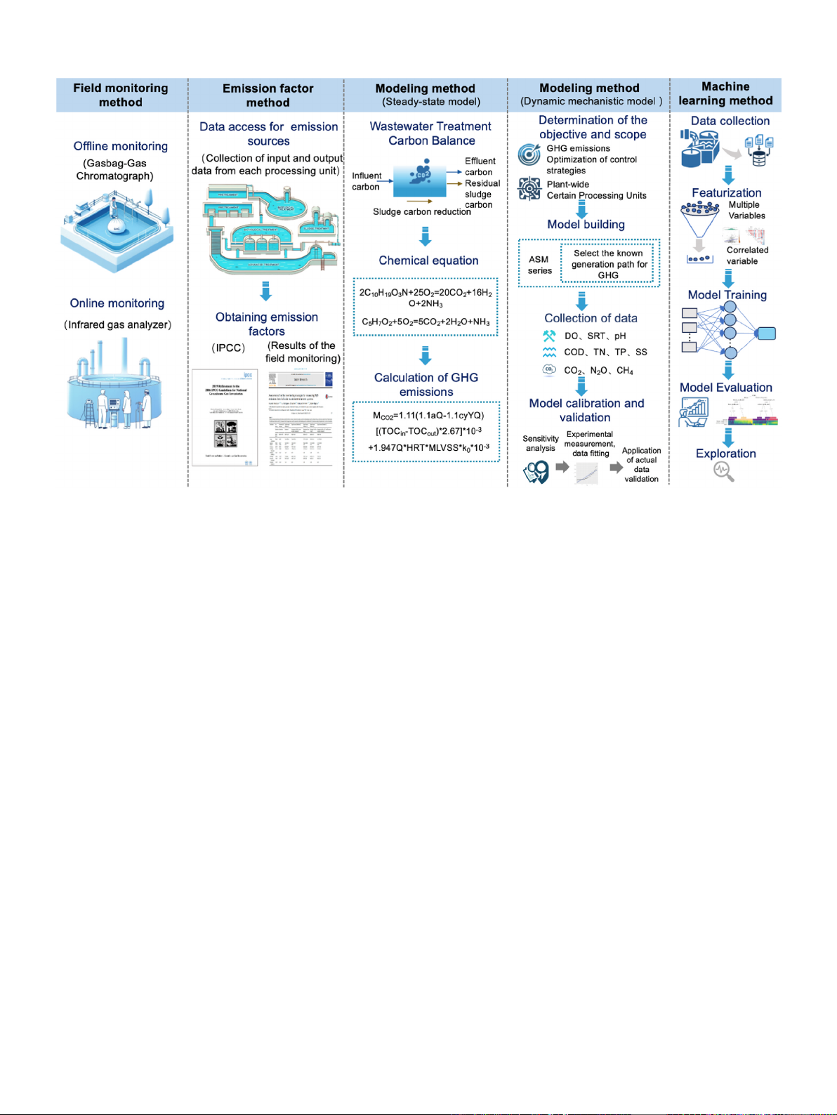
2. Methodologies of GHG emissions accounting
With each section outlining the features and operational procedures
of the various methods, Fig. 1 illustrates how the emission factor
method, the field monitoring method, the modeling methods, and the
machine learning method account for GHG emissions from WWTPs.
2.1. Field monitoring method
Field monitoring methods obtain GHG emission results by collecting
and analyzing data in situ. At present, there are offline monitoring and
online monitoring methods. The offline monitoring method involves
collecting gas samples in a designated area using airbags (Foley et al.,
2010) and static boxes and then using gas chromatography in the lab-
oratory to determine the gas samples (Parvan et al., 2020). This method
is manually conducted; consequently, the sample collection and pro-
cessing is characterized by numerous challenges, such as poor sample
representativeness and measurement accuracy. These challenges can
interfere with the results, further decreasing the accurate capturing of
greenhouse gas emissions and the evolution time (Vasilaki et al., 2019).
The online monitory method is more commonly used to monitor carbon
emissions using infrared gas analyzers and microelectrode sensors.
These devices can inscribe second-granularity time-series carbon
L. Huang et al.
Journal of Cleaner Production 448 (2024) 141424
3
emission inventories but are expensive (Liu et al., 2014). In addition,
they are suitable for monitoring emission sources in small areas to study
the characteristics of GHG emissions. Information on specific methods is
detailed in Supplementary Information Table S1.
In the early nineties, as the global climate change problem gradually
attracted attention, the GHG emissions during the wastewater treatment
process were also taken into account to mainly monitor the GHG emis-
sions produced in activated sludge (Bruins et al., 1995; Czepiel et al.,
1993; Sfimer and Weiske, 1995). Subsequently, offline monitoring
methods have been mainly used since the 21st century to understand the
emission mechanism of GHG in different processes (Aboobakar et al.,
2013; Kampschreur et al., 2008; Liu et al., 2009; Ren et al., 2013; Ye
et al., 2014). In addition, offline monitoring methods are mainly to
assess the effects of different operating conditions, design parameters,
and environmental factors (e.g., temperature, pH, and oxygen concen-
tration) on GHG emissions (Baresel et al., 2016; Daelman et al., 2015;
Pascale et al., 2017; Rong et al., 2023). However, these methods are only
applied in enclosed sites or enclosed WWTPs with ventilation systems
(Samuelsson et al., 2018). In the past decade, devices, including infrared
gas analyzers, microelectrode sensors, and remote sensing, have been
applied to real-time monitoring of GHG emissions in WWTPs
(Samuelsson et al., 2018). These efforts aim to explore ways of achieving
a balance between enhancing operational efficiency and conserving
energy without increasing GHG emissions (Aboobakar et al., 2013).
Furthermore, these devices can provide spatial and daily variability data
to investigate the impacts of sudden parameter changes on GHG emis-
sions (Jia et al., 2019; Ribera-Guardia et al., 2019).
2.2. Emission factor method
The emission factor method involves the multiplication of the ac-
tivity data by the emission factor to estimate carbon emissions from
various emission sources:
Emissions =AD ×EF ×GWP (1)
Where Emissions represent the mass flux of GHG released into the at-
mosphere for one year, kg CO
2
-eq/yr. AD stands for activity data, which
refers to the specific usage and input quantities directly related to carbon
emissions from an individual emission source within one year. EF is the
emission factor (the amount of greenhouse gases emitted per unit of use
of a given source) and GWP is the global warming potential (the relative
radiative impact of a given substance compared to carbon dioxide over a
given time-integrated range). Emission factors can be adopted from
recommended valuable resources, including IPCC reports, international
emission factor databases, national lifecycle inventory data, journal data
from public reports, and other specific research outputs (such as census,
survey, and monitoring data).
The emission factor method can not only calculate the CO
2
, CH
4
, and
N
2
O emissions generated during the wastewater treatment process but
also calculate the indirect GHG emissions caused by electricity, chemical
agents, and transportation consumption. The commonly adopted
method for calculating indirect GHG emissions at present is the emis-
sions factor method (Chai et al., 2015; Maktabifard et al., 2022a; Pang
et al., 2022; Wu et al., 2022; Zib et al., 2021). This involves taking into
account factors such as electricity consumption, chemical usage, and
transportation distances, and then multiplying them by the respective
emissions factors to obtain the results.
Before the adoption of the IPCC’s approach to emission factors, the
researchers conducted preliminary measurements and data collection on
GHG emissions using field monitoring methods. Based on extensive
measurements and studies, some scientists began to establish GHG
emission factors for specific processes in wastewater treatment, such as
N
2
O emissions from nitrification-denitrification and CH
4
from anaerobic
digestion process (Bruins et al., 1995; Cakir and Stenstrom, 2005;
Fig. 1. Procedures of different GHG emission accounting methods. The steady-state model for aerobic wastewater treatment system is depicted in the figure and the
GHG emission model for anaerobic wastewater treatment system can be referred to the study of Cikar et al. (2005). c: constant, oxygen equivalent of bacterial cells;
2.67: the amount of oxygen needed to consume one TOC unit; TOC
in
: total carbon content at the inlet of the aerobic tank; TOC
out
: total carbon content at the outlet of
the aerobic tank; MLVSS: mixed liquor volatile suspended solids; y: MLVSS/MLSS; Y: sludge yield coefficient.
L. Huang et al.

Journal of Cleaner Production 448 (2024) 141424
4
Kampschreur et al., 2008; Sfimer and Weiske, 1995). Subsequently,
research on emission factors has become more comprehensive and sys-
tematic on a global scale. In 2006, the IPCC formally released the 2006
IPCC Guidelines for National Greenhouse Gas Inventories and provided
detailed accounting methods and an emission factor inventory (IPCC,
2006). Building on the previous foundation, the IPCC released added
accounting methods for N
2
O emissions from industrial wastewater
treatment and the corresponding emission factors, among other content
(IPCC, 2019). However, some studies did not adopt the recommended
values provided by the IPCC inventory guidelines because the guidelines
offer general methods and default emission factors that do not apply to
most situations and countries (Maktabifard et al., 2022a; Marinelli et al.,
2021). Khalil et al. (2023) found that the N
2
O emission factor provided
by the IPCC in 2019 was 3–4 times that of the emission factor measured
using sensors at a Danish WWTP.
2.3. Modeling method
The modeling method is based on the wastewater treatment process
and involves using various parameters and variables to simulate GHG
emissions under different scenarios (Henze et al., 2015; Lu et al., 2023;
Solís et al., 2022). The commonly used models for calculating green-
house gas emissions include steady-state and dynamic mechanistic
models.
2.3.1. Steady-state model
The steady-state model is based on the principle of mass balance,
which entails subtracting the content of the output material from the
content of the input material to obtain the emission equivalent. In
wastewater treatment, the operating state is often considered a steady
state, with the fugitive GHG equal to the carbon content in the influent
minus the carbon content in the effluent and the effluent sludge. Steady-
state models are commonly used to calculate CO
2
and CH
4
produced
through biological treatment processes. Although the main pathways for
the GHG in wastewater treatment have not been identified, an accurate
carbon emission model can be established based on the wastewater
treatment process and combined with the mass balance, stoichiometric
equations, and on-site energy and material consumption (Bani Shaha-
badi et al., 2010). Monteith et al. (2005) used this idea to design a GHG
emission model for WWTPs in Canada and found that the GHG emissions
from the conventional activated sludge method were 0.26 kg
CO
2
-eq/m
3
. Cakir and Stenstrom (2005) modeled the CO
2
and CH
4
emissions in anaerobic wastewater treatment systems and investigated
the differences from aerobic wastewater treatment systems, the analysis
shows that for very low strength wastewater (less than 300 mg/L BOD
u
),
aerobic processes will emit less GHG emissions. Bani Shahabadi et al.
(2009) assessed CO
2
and CH
4
emissions from aerobic, anaerobic, and
mixed treatments based on specific kinetic relationships and mass bal-
ances, the overall on-site emissions were 1952, 1992, and 2435 kg
CO
2
-eq/d. Gori et al. (2011) proposed a simplified model based on COD
equilibrium and biochemical reaction equations to analyze the effect of
COD and primary sedimentation tanks on the carbon and energy foot-
prints of WWTPs. The result shows that an increase in the proportion of
soluble COD increases carbon emissions and energy demand, and an
increase in particulate COD decreases. However, an unintended removal
of COD may be required for downstream nutrients. Gori et al. (2013)
used the Activated Sludge Model No. 3 (ASM3) by Henze et al. (2015)
and the Anaerobic Digestion Model 1 (ADM1) by Batstone et al. (2002)
to couple the active sludge and digestion processes. They discussed the
role of primary sedimentation tanks in energy recovery and carbon
footprint, demonstrating the interconnections and interactions between
treatment units.
The development of steady-state models has continuously evolved,
providing important references for GHG emissions in the wastewater
treatment sector. For instance, Koutsou et al. (2018) used the
steady-state model to study the on-site and off-site GHG emissions of 220
WWTPs in Greece. Iqbal et al. (2020) combined the steady-state model
with life cycle assessment (LCA) to examine the impact of treating food
waste at Hong Kong’s largest wastewater treatment facility, including
design, operational capacity, and GHG emissions. Zhang et al. (2021)
established a comprehensive steady-state model for energy saving and
emission reduction in urban wastewater treatment systems based on
carbon emissions, used for calculating the effects of energy saving and
emission reduction and their impact on environmental carbon
emissions.
2.3.2. Dynamic mechanistic model
Based on the biochemical reaction process and kinetics of substances
in wastewater, the dynamic mechanistic model describes the impact of
different control strategies (including operating conditions and water
inflow) on greenhouse gas emissions by obtaining experimental data,
calibrating the model, and exploring the greenhouse gas formation
process. Moreover, the dynamic mechanistic model can be evaluated at
the activated sludge treatment unit level and applied to the whole plant
while considering their interactions, which is important for assessing the
N
2
O of WWTPs.
An in-depth understanding of the emission pathways of N
2
O has
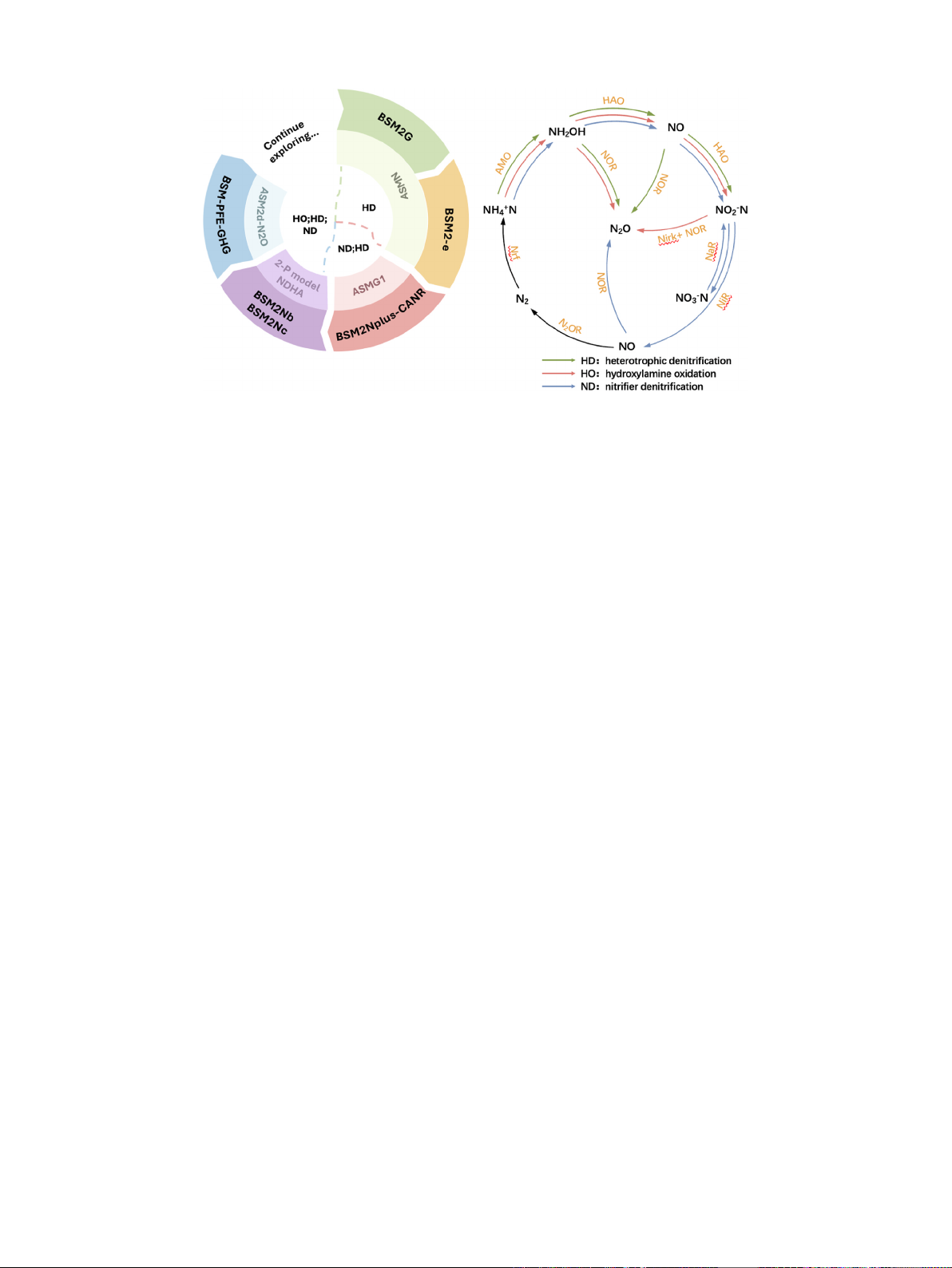
facilitated the ongoing development of dynamic mechanistic models.
The development of related models and the N
2
O generation paths are
shown in Fig. 2.
Hiatt and Grady (2008) introduced the Activated Sludge Model for
Nitrogen (ASMN), which accounted for intermediate products (such as
nitrite, nitric oxide, and nitrous oxide) produced during nitrification and
denitrification processes, previously overlooked in traditional activated
sludge models. They modeled the denitrification process using four
separate rate equations, enabling more accurate calculations of N
2
O
production. Samie et al. (2011) found that the half-saturation co-
efficients for electron acceptors and donors, as well as the oxygen in-
hibition coefficients in the Activated Sludge Model for Nitrogen
(ASMN), were derived from reference literature and the Activated
Sludge Model No. 1 (ASM1). They modified ASM1 to simulate N
2
O
production in the four-step denitrification process, and calibrated the
model at a wastewater treatment plant in Paris, France, over a year,
resulting in a simulated average N
2
O emission of 4.95 kg N
2
O–N/d,
consistent with experimental estimates. Ni et al. (2011, 2013), recog-
nizing the lack of in-depth understanding of N
2
O production driven by
ammonia-oxidizing bacteria (AOB) in previous studies, simulated the
dynamic changes of N
2
O during the autotrophic nitrification process of
AOB and the incomplete oxidation process of hydroxylamine.
As research into nitrogen metabolism deepened, the mechanisms of
N
2
O production were investigated, and subsequent studies have started
to integrate singular pathways to enhance the accuracy of N
2
O predic-
tion. Guo and Vanrolleghem (2014) combined the AOB denitrification
model proposed by Mampaey et al. (2013) with ASMN to establish the
Activated Sludge Model for Greenhouse Gas No. 1 (ASMG1). Through
calibration and validation, ASMG1 was refined to more accurately
predict the N
2
O emissions under different temperatures and control
strategies. Domingo-F´
elez and Smets (2016) combined biological (hy-
droxylamine oxidation, autotrophic denitrification, and heterotrophic
denitrification) and abiotic pathways (chemical reactions driven by
NH
2
OH) to establish an integrated model (NDHA). Pocquet et al. (2016)
integrated hydroxylamine oxidation and autotrophic denitrification
pathways to establish a dual-path model for AOB (2-P model). Massara
et al. (2018) developed the Activated Sludge Model 2 d - Nitrous Oxide
(ASM2d-N
2
O), which incorporates biological pathways (AOB
nitrification-denitrification, hydroxylamine oxidation, and heterotro-
phic denitrification). This model can describe N
2
O emissions from urban
WWTPs under dynamic conditions and offers in-depth insights into the
impact of dissolved oxygen (DO) on nitrification processes and N
2
O
emissions. The simulations indicate that at high DO levels (>3 mg/L),
the N
2
O emission factor significantly decreases, falling below 2%. High
DO levels are beneficial in reducing N
2
O emissions, but this comes with
L. Huang et al.
Journal of Cleaner Production 448 (2024) 141424
5
a corresponding increase in energy consumption.
In wastewater treatment systems, N
2
O is primarily produced during
the biological nitrogen removal process, especially in the nitrification-
denitrification by AOB, hydroxylamine oxidation, and heterotrophic
denitrification processes. Subsequently, N
2
O is emitted into the atmo-
sphere from the water-air interface. N
2
O is a gas relatively soluble in
water and, in the absence of active stripping (the process of removing
gas from liquid), can accumulate in water to relatively high concentra-
tions (Weiss and Price, 1980). Law et al. (2011) noted that intense
aeration processes enhance the activity of nitrifying bacteria, leading to
the stripping of dissolved N
2
O from the water phase. In dynamic
mechanistic models, the gas stripping equation (Foley et al., 2010) or the
gas emission rate (Schulthess and Gujer, 1996) can calculate the transfer
of gases from the liquid phase to the gas phase. The gas stripping models
have evolved over time. Foley et al. (2010) proposed a simplified N
2
O
stripping equation based on the principles of liquid-gas mass transfer.
Additionally, Flores-Alsina et al. (2011) incorporated this stripping
equation into the BSM2G model to simulate N
2
O emissions. Moreover,
Massara et al. (2018) introduced a stripping effectiveness coefficient to
the stripping equation established by Foley et al. (2010). This involved
setting different stripping effectiveness factors under various conditions
to assess their impact on N
2
O emissions. The N
2
O emission rate, pro-
posed by Schulthess and Gujer (1996), has been widely adopted
(Blomberg et al., 2018; Guo and Vanrolleghem, 2014) and includes
methods for calculating emissions in aerated and non-aerated zones. The
volumetric oxygen transfer coefficient (KLa) in both the stripping
equation and gas emission rate is a key factor influencing liquid-gas
transfer outcomes. KLa can be determined through various methods
including the surface gas velocity method (Foley et al., 2010), empirical
approaches based on the Higbie penetration model (Khudenko and
Shpirt, 1986), the empirical method of Dudley (1995), and the oxygen
transfer rate method (Massara et al., 2018).
To assess the impact of different control strategies on GHG emissions,
Benchmark Simulation Models (BSMs) have incorporated GHG emis-
sions as a performance indicator and underwent a series of enhance-
ments (such as improving the dynamic simulation of N
2
O) to more
accurately describe GHG emissions under various strategies. For
example, Flores-Alsina et al. (2011) for the first time incorporated GHG
emissions into a plant-wide dynamic mechanistic model by proposing
Benchmark Simulation Model no. 2 Greenhouse gas (BSM2G) that pre-
dicts the production of N
2
O by heterotrophic denitrifying bacteria,
BSM2G is based on the simulation of ASMN and ADM1 for 4 step
denitrification of N
2
O and the dynamic production of CO
2
and CH
4
from
anaerobic digestion of sludge. The diffusive emissions estimation model
(DEEM) model proposed by Rodriguez-Garcia et al. (2012), considers
the possibility of converting NO
2
to N
2
O through heterogeneous deni-
trification and also the accumulation of N
2
O by NO-related inhibition in
heterotrophic denitrification, was applied to assess the GHG emissions
in WWTPs in Spain. In addition, the DEEM model can be easily applied
to LCA compared with the other models. Because the DEEM model ap-
plies the ASMN and activated sludge/anaerobic digestion models and
considers sufficient design and operating parameters, it is possible to
fully estimate the CO
2
, CH
4
, and N
2
O emissions of each structure and
provide critical environmental impact data for life cycle assessment.
Sweetapple et al. (2013) proposed the Benchmark Simulation Model
No.2-extended (BSM2-e) to analyze parameter sensitivity. In the appli-
cation of BSM2-e, the main sources of uncertainty in direct N
2
O emis-
sions were found to include half-saturation coefficients for nitrate, NO
2,
and NO reduction by biodegradable substrates, and further reductions in
the uncertainty in the values of these parameters would help to reduce
the uncertainty in total GHG emissions.
In considering greenhouse gas (GHG) emissions from novel biolog-
ical nitrogen removal processes, Boiocchi et al. (2015) proposed the
Benchmark Simulation Model No.2 for Nitrous Oxide and Complete
Autotrophic Nitrogen Removal (BSM2NplusCANR). This model in-
tegrates the mainstream process of ASMG1 with the sidestream process
of Complete Autotrophic Nitrogen Removal (CANR) (Vangsgaard et al.,
2012) to describe both mainstream and sidestream partial nitritatio-
n/Anammox (PN/A) wastewater treatment processes. The results indi-
cate that the strategy for controlling N
2
O production in mainstream
processes can focus on the activity of AOB. The adoption of a new PN/A
reactor can increase the total nitrogen removal efficiency by approxi-
mately 10% and save about 16% of the oxygen demand (Boiocchi et al.,
2015). Boiocchi et al. (2017) developed three models: Benchmark
Simulation Model No. 2 for Nitrous Oxide a (BSM2Na), Benchmark
Simulation Model No. 2 for Nitrous Oxide (BSM2Nb), and Benchmark
Simulation Model No. 2 for Nitrous Oxide c (BSM2Nc), based on the
ASMG1, the 2-P Model, and the NDHA. These models were designed to
Fig. 2. Dynamic mechanistic model and N
2
O generation path. Note: (i) The figure on the left shows the development of a model of the dynamic mechanistic of
greenhouse gases clockwise. (ii) HD represents the pathways of N
2
O production simulated with ASMN. ASMN is a sub-model included in models BSM2G and BSM2-e.
ND and HD represent the pathways of N
2
O production simulated by ASMG1. ASMG1 is a sub-model in the BSM2Nplus-CANR. HO, HD, and ND are the pathways of
N
2
O production simulated using the 2 P-model, NDHA, ASM2d-N
2
O. The 2 P-model and NDHA are sub-models of BSM2Nb and BSM2Nc, respectively. ASM2d-N
2
O is
a sub-model within the BSM-PFE-GHG model. (iii) AMO: ammonia monooxygenase, HAO: hydroxylamine oxidoreductase, NOR: nitrite oxidoreductase, NOB: nitrite-
oxidizing bacteria, Nirk: copper-containing nitrite reductase, NaR: membrane-bound nitrate reductase, Nrf: cytochrome c nitrite reductase, Nod: nitric
oxide dismutase.
L. Huang et al.


![Công nghệ xử lý bụi: Tìm hiểu về các công nghệ [Mới nhất]](https://cdn.tailieu.vn/images/document/thumbnail/2013/20130712/sunshine_5/135x160/5501373640741.jpg)