REGULAR ARTICLE
Hydraulic and statistical study of metastable phenomena
in PWR rod bundles
Florian Muller
*
CEA Saclay, DEN/DANS/DM2S/STMF/LMSF, 91191 Gif-sur-Yvette, France
Received: 30 October 2019 / Accepted: 15 November 2019
Abstract. The analysis of fuel rod bundle ows constitutes a key element of Pressurized-Water Reactors
(PWR) safety studies. The present work aims at improving our understanding of nefarious reorganisation
phenomena observed by numerous studies in the ow large-scale structures. 3D simulations allowed identifying
two distinct reorganisations consisting in a sign change for either a transverse velocity in rod-to-rod gaps or for a
subchannel vortex. A Taylor frozen turbulencehypothesis was adopted to model the evolution of large-scale
3D structures as transported-2D. A statistical method was applied to the 2D eld to determine its
thermodynamically stable states through an optimization problem. Similarities were obtained between the
PWR coherent structures and the stable states in a simplied 2D geometry. Further, 2D simulations allowed
identifying two possible ow bifurcations, each related to one of the reorganisations observed in 3D simulations,
laying the foundations for a physical explanation of this phenomenon.
1 Introduction
Insufcient ow thermal mixing in the rod bundles within a
Pressurized-Water Reactor (PWR) can lead to a boiling
crisis, which is nefarious for the reactor operational safety.
Mixing grids are typically used to enhance the thermal
mixing inside fuel arrays, mostly through the intensica-
tion of the secondary ows. These secondary ows have a
tendency to organize into large-scale structures in the plane
normal to the tube axes. Numerous experimental or
numerical studies have shown the existence of reorganisa-
tion phenomena in the transverse ow large-scale struc-
tures (see the review in appendix A from Kang and Hassan
[1]). In particular, the AGATE experimental results [2]
featured a global 90°rotation of the cross-ow pattern
between the near and the far wake of a mixing grid. This
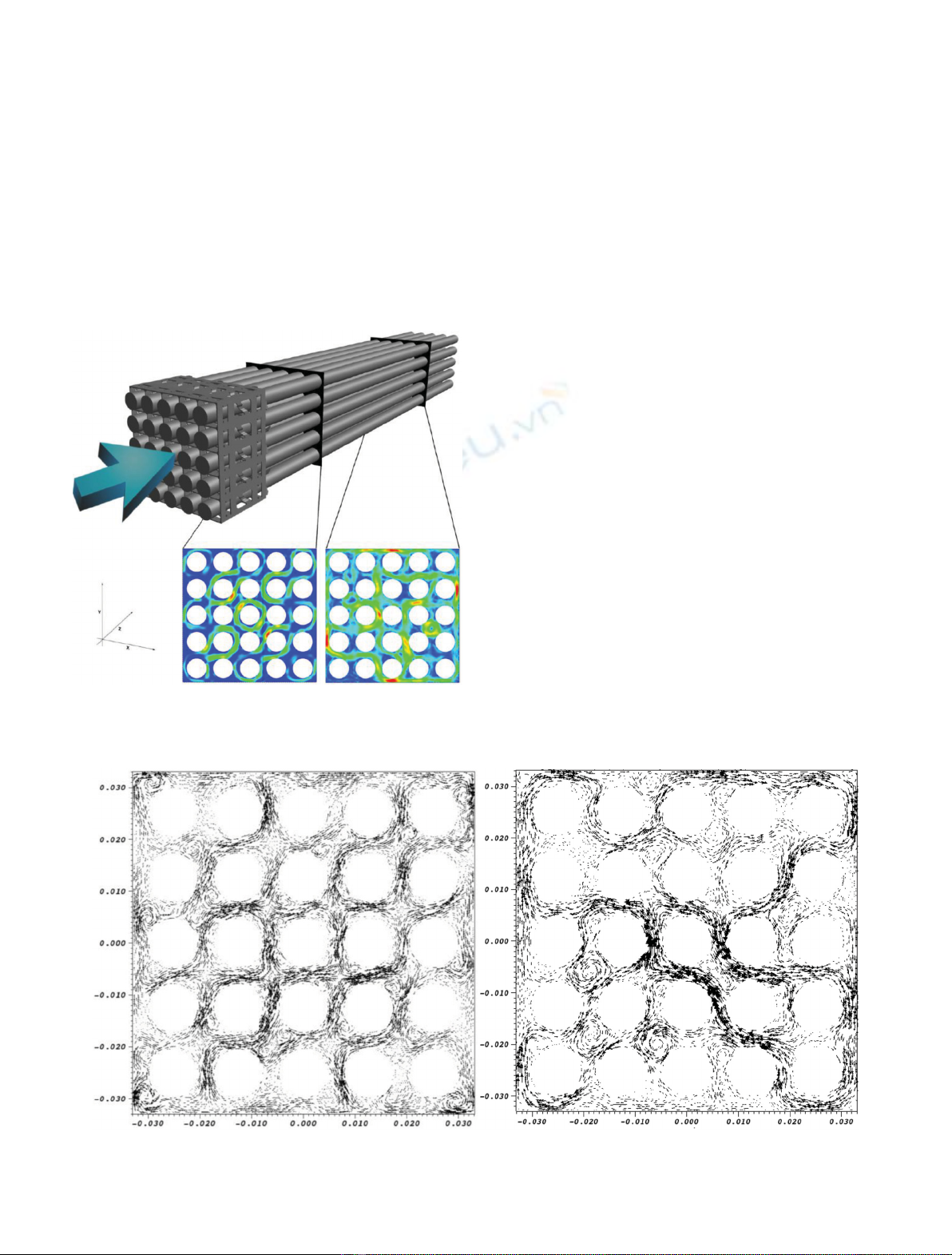
reorganisation is shown in Figure 1: a sketch of a 5 5 rod
bundle tted with a mixing grid, as well as colour plots of
the transverse ow downstream a mixing grid are shown.
The cross-ow is aligned with a 45°angle in the rst one,
but has rotated by 90°in the second one.
Such reorganisations are very signicant for reactor
safety studies: due to the points with zero cross-ow they
induce, they lead to drops in the thermal mixing as
demonstrated by Shen et al. [3], which can pose a serious
risk to the PWR reactor operational safety. This work
aimed at improving our understanding of these phenomena,
both for enhancing their characterization and for identifying
their origin, with the long-term goal of developing small-scales
models suited for this type of ow.
Little concrete information can be found in the
literature on the reorganisation phenomenon. This is due
to the lack of high-quality experiment where the
phenomenon typically occurs, and to the fact that, among
the variety of Computational-Fluid Dynamics (CFD)
numerical simulations performed for rod bundle ows,
few were conducted for the entire rod bundle axial span and
with high-delity turbulence models. Attempting a new
method, we focused on a physical approach to the
reorganisation phenomenon by proposing an original
method for the study of the rod bundle ow. A similarity
was noticed between PWR rod bundle ow reorganisations
and some phenomena typically experienced by quasi-2D
geophysical ows, such as the Jupiter Red Spot or the Gulf
Stream [4]. Indeed, the latter sometimes display important
changes in their structure, leading to oscillations between
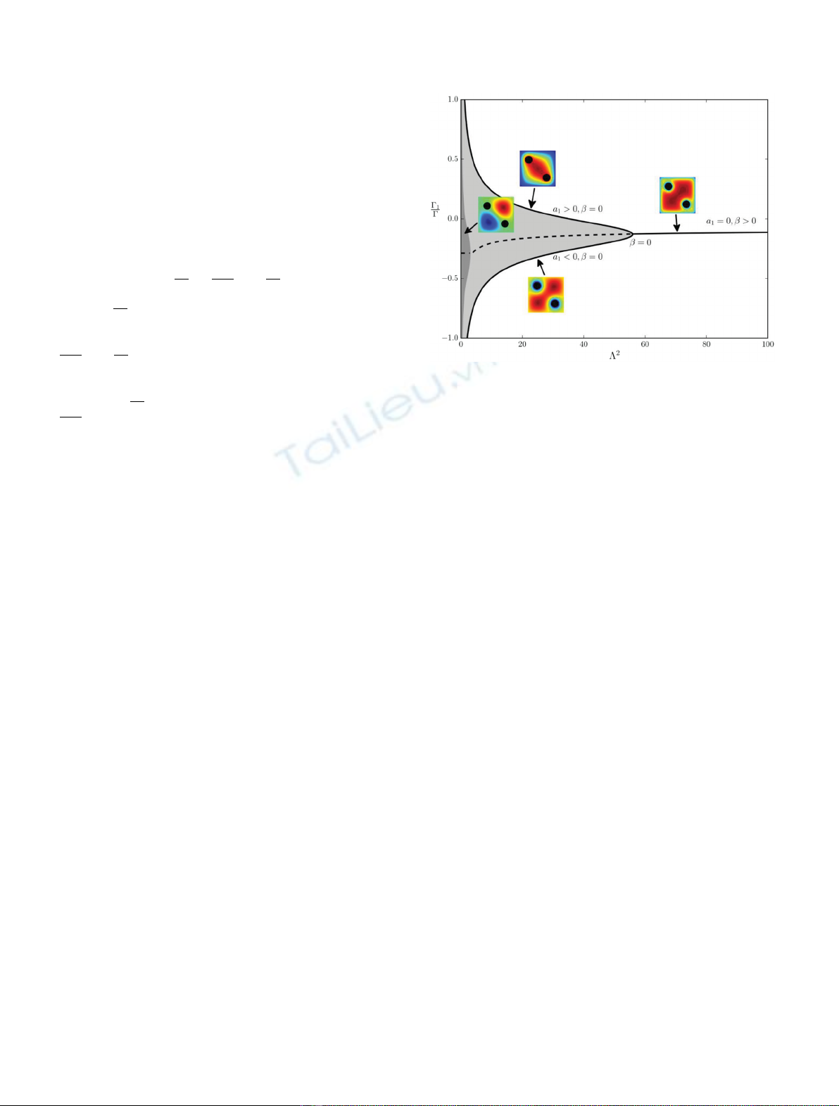
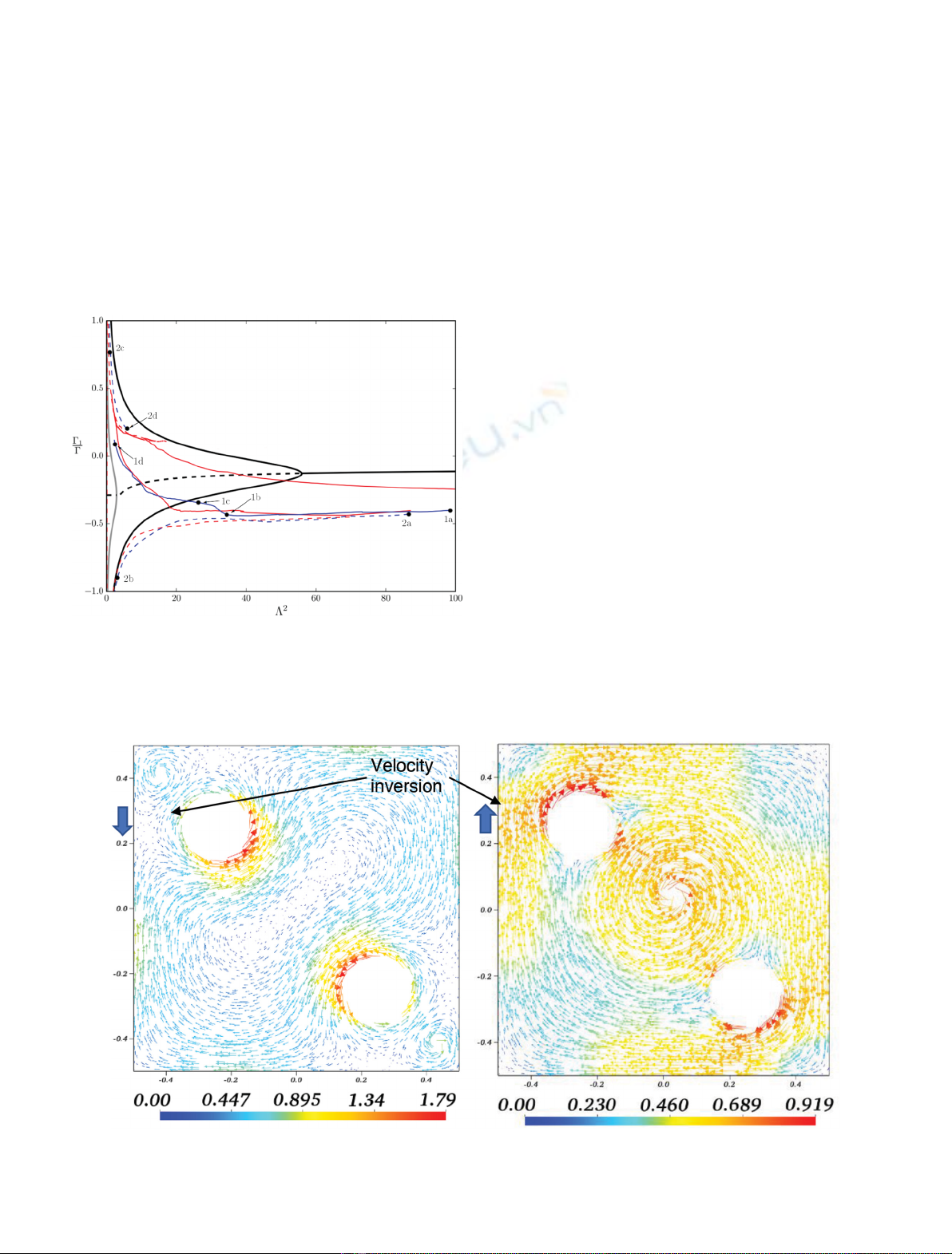
very distinct solutions. These phenomena can be inter-
preted as phase transitions between different equilibrium
states which become metastable.
In order to study the reorganisation phenomena from
the perspective of this similarity with 2D ows, the following
steps were taken. 3D simulations were rst performed in
order to decompose the large-scale reorganisations into
local inversions, and to justify a Taylor frozen turbulence
hypothesis, as described in Section 2.Section 3 details the
2D statistical method that was applied in simplied
geometries with obstacles based on this hypothesis. The
*e-mail: orian.muller99@gmail.com
EPJ Nuclear Sci. Technol. 6, 6 (2020)
©F. Muller, published by EDP Sciences, 2020
https://doi.org/10.1051/epjn/2019057
Nuclear
Sciences
& Technologies
Available online at:
https://www.epj-n.org
This is an Open Access article distributed under the terms of the Creative Commons Attribution License (https://creativecommons.org/licenses/by/4.0),
which permits unrestricted use, distribution, and reproduction in any medium, provided the original work is properly cited.
stable states obtained through this method are then used
in 2D free decay simulations in Section 4, highlighting
similarities between their phase transitions and the 3D
reorganisation phenomenon. Section 5 provides a conclu-
sion on the physicality of the reorganisation phenomenon.
2 3D CFD simulations
We performed 3D CFD simulations in rod bundles using
the TrioCFD [5] code along with a WALE sub-grid scale
turbulence model, in a tetrahedral mesh of 34.4 million cells
and using in parallel 1000 CPU cores. Details on the
numerical performance of this code were discussed by
Angeli et al. [6]. The ow was characterized by a Reynolds
number Re = 96 000. Cross-ow reorganisations were
observed in the simulation results, as depicted in Figure 2:
the averaged transverse ow at 30 mm downstream the
mixing grid in the rst plot displays a 45°orientation, while
that at 150 mm in the second plot is aligned with the 135°
diagonal. A signicant impact of the numerical schemes
used was also noted, which is a topic still under
investigation by the community. Most importantly, we
could distinguish two particular types of local cross-ow
reorganisations.
The cross-ow can undergo an inversion of the
transverse velocity between two rods, or a sign change
for a vortex in the centre of a subchannel (the vacant space
between four rods). Different combinations of velocity
inversionsaround a subchannel (e.g. one to four
inversions) can lead to a variety of pattern changes, one
of which is a global 90°rotation of the cross-ow pattern.
This type of inversion was already noted in previous work
by Shen et al. [3].
Besides, we also observed in the 3D simulation results
multiple sub-channels featuring a cross-ow pattern
change without any gap ow inversion. Instead, the
circulation inside these sub-channels seemed to vary
greatly. This increase consisted either in a sign change
for the subchannel vortex if one was present, or the
apparition of a vortex in a pure shear ow. One of the
possible large-scale pattern changes obtained was the 90°
rotation of the subchannel cross-ow pattern.
Remarkably, the same nal patterns can be obtained
after each of these two reorganisations through two
different ow evolutions, providing a more nuanced view
of the possible reorganisations in rod bundle cross-ows.
Fig. 1. Sketch of a rod bundle and colour plots of the transverse
velocity eld downstream the mixing grid.
Fig. 2. Averaged transverse velocity eld from a LES simulation of the ow in a 5 5 rods fuel assembly, at 30 mm (left) and 150 mm
(right) downstream a mixing grid.
2 F. Muller: EPJ Nuclear Sci. Technol. 6, 6 (2020)
In order to tackle the reorganisation phenomenon, it
was decided to adopt an approach based on a statistical
uid mechanics point of view and relying on a Taylor
frozen turbulencehypothesis. This hypothesis is com-
monly used in meteorological ows (see Higgins et al. [7])
where local turbulent eddies are advected by a mean wind
and are considered frozenat a xed position. Under this
hypothesis, one can consider that a rod bundle cross-ow
behaves as a quasi-2D ow transported by the axial
component of the velocity eld. This hypothesis allows
decomposing the 3D velocity eld u(x,y,z,t) into:
ux;y;z;tðÞ¼
uzzþux;yx;y;uztðÞþu0x;y;z;tðÞ:
Here uzis a uniform axial component, and u
0
(x,y,z,t)
denotes the 3D turbulent uctuations. The (x,y)
components form a purely advected transverse 2D part
ux;yx;y;uztðÞthat is assumed to abide by the 2D Navier
Stokes equations. In order to verify this hypothesis, the
ow must display very small variations of the axial
component uzcompared to that of the transverse ow eld
ux;y, and a high scale difference between the axial and
transverse components.
These criteria were mostly fullled outside of boundary
layers and past the near wake of the mixing grid, notably
with a scale ratio between the axial and transverse
components of up to 30. Although deviations from the
hypothesis are observed and should be investigated further,
such a decomposition allowed us to apply statistical
methods inspired by geophysical ow studies to the
transverse 2D part.
3 2D statistical approach
Past studies on 2D turbulent ows through the lens of
statistical uid mechanics have tackled a broad set of
physical elds, from thin oceanic layers to the Red Spot in
the Jovian atmosphere and experimental soap lms. A
crucial part of the study of such 2D ows is the prediction of
the steady stable structures emerging from given initial
characteristics and depending on the domain geometry. In
the framework of PWR rod bundle ows, this prediction
consists in the determination of stable patterns for the
transverse ow, following initial conditionsset by its
passage through the mixing grid.
Instead of an exhaustive application of a dynamical
stability criterion to the innite set of steady solutions to
the 2D Euler equations, an equivalence can be used
between such a dynamical stability criterion and a
constrained optimization problem, usually on a measure
of the entropy with conservation of a varying set of Euler
invariants, following the work from Miller et al. [8,9]. This
allows for the use of several tools coming from mathemati-
cal optimization theory, and to directly calculate the
expected steady state in a given 2D physical conguration.
Multiple theories have been devised to determine these
stable states, leading to various constrained optimization
problems. We have focused on the Minimum-Enstrophy-
Principle (MEP) due to its relative simplicity and the
linear equations it leads to. This principle was proposed
from phenomenological considerations (see Bretherton and
Haidvogel [10]), and it states that the stable ow regimes
minimize the enstrophy of the system under constant
energy and circulation. The enstrophy is dened as
G2¼
V
v2dr, with vthe ow vorticity eld and Vthe
physical domain.
A resolution method for this problem was devised and
proposed by Naso et al. [11], applicable to simply-
connected domain geometries. We adapted this method
to geometrical domains with internal obstacles in order to
allow the consideration of typical rod bundle cross-section
geometries. Each obstacle adds the conservation of the ow
circulation around itself and thus another degree of
freedom to the problem.
The minimization of the enstrophy under multiple
constraints leads to a variational problem solved in our
method through a projection on the Laplace eigenbasis.
Scanning the parameter space and interpolating for
constant energy, circulation and circulation around the
obstacles allows determining the stable solutions for any
combination of the integral constraints. Details on the
derivation of the solutions and on the method followed to
explore the solution ensemble are available in Muller et al.
[12].
Our method has been validated rst through numerical
convergence studies and recovery of literature results [13],
before being applied in the case of a square domain with
two diagonally opposed obstacles. This simple geometry
was designed as a basic model for a PWR rod bundle cross-
section. In order to reduce the number of degrees of freedom
in the problem, we assumed equal circulations around the
two obstacles, justied by the typical cross-ow patterns
observed downstream mixing grids in PWR rod bundle
ows and shown in Figure 1.
This approach resulted in the stability map shown in
Figure 3. Therein, L
2
=G
2
/(2E) with Ethe total ow
energy combines the energy and circulation into one
Fig. 3. Stability map obtained in a square geometry with two
obstacles, following the application of the Minimum-Enstrophy
Principle. Depending on the value of the parameter L
2
, one or two
ow regimes can be stable in the domain.
F. Muller: EPJ Nuclear Sci. Technol. 6, 6 (2020) 3
parameter, while G
1
is the circulation around the obstacles
in this geometry. The thick black line indicates the
minimal-enstrophy state, solution of our multiply-
constrained optimization problem. Under the MEP, this
solution is a stable ow for given values of the parameters
(G,E,G
1
). The light and dark grey areas, respectively,
indicate areas of lower-enstrophy for 1- and 2-vortices
solutions, but their enstrophy is systematically higher than
that of the solutions on the black line. In the graph, bis
related to the energy Eand a
1
to the boundary condition on
the obstacles. Interestingly, a single solution is stable
forL2>L2
crit, while two branches are stable forL2<L2
crit.
Further, the single branch features a central vortex aligned
with the diagonal without obstacles and one vortex around
each obstacle, while the upper branch for L2<L2
crit
displays a single vortex around both obstacles on the
opposite diagonal.
Therefore, two stable regimes differing by a 90°angle
were obtained, which recalls the pattern reorganisations
observed in PWR rod bundle cross-ows. Although in the
2D statistical approach, the parameters (G,E,G
1
) are xed
due to their conservation by the Euler equations, they can
be dissipated by viscosity in physical systems, leading to
changes in the minimal-enstrophy solution and thus stable
states. Phase transitions can thus occur between these
states, which were investigated further in our study.
4 2D free-decay CFD simulations
To further validate the methodology and the computa-
tional code for the statistical approach and check if a link
could be established between the statistical approach and
the CFD calculations, the case of the free relaxation of
turbulent 2D ows has been studied afterwards. The
objective was to compare the ow reached in the long-run
of a 2D CFD simulation and the stable state predicted by
the statistical approach, from initial conditions either
random or designed to investigate particular ow regimes.
The simulations were set up to feature as little diffusion
as possible in order to conserve energy relatively well when
compared to the spontaneous enstrophy dissipation.
Similarly to the 3D simulations, the 2D simulations
conducted in this study were based on the code TrioCFD
[5]. They did not use any turbulence model. In order to
allow the capture of most ow scales, moderate Reynolds
numbers were chosen (Re = 3000). When choosing the
numerical schemes, we opted as much as possible for the
less dissipative ones: only slightly upstream convection
schemes, a third-order Runge-Kutta time advancement
method and a resolution of the pressure equation through a
Cholesky method [6]. Regarding the boundary conditions,
we used stress-freeboundary conditions, which in
practice amounted to a nullity condition on the normal
velocity component at the boundary. We found this
method to be the closest one to the physical framework of
the statistical approach, where the existence of a non-zero
circulation G
1
around the internal obstacles requires in turn
the tangential velocity at the boundary of the obstacles to
be non-zero.
We rst validated the process by recovering nal states
in square and rectangular domain geometries in accordance
with statistical mechanics literature results, and by
capturing plausible turbulent cascades for the kinetic
energy. The decay process obtained in a square geometry is
shown in Figure 4. In this geometry, the Minimum-
Enstrophy Principle approach (see Chavanis et al. [13])
leads to a single central vortex as the only stable solution.
Having initiated our simulation with an array of Taylor-
Green vortices, it underwent a phase of strong mixing,
before converging towards the expected single-vortex
stable state.
In the case of the square domain with two obstacles, the
simulations were tailored to have initial conditions
spanning the (L
2
,G
1
/G) parameter space. This was
performed through the initialization of the simulations
with carefully designed analytical functions. Let (O, e
r
,e
u
)
dene a polar coordinate system with O the square center
as origin point, e
r
a unitary vector along the position vector
rand e
u
a unitary vector orthogonal to r. The analytical
functions for the simulation initial conditions were built
through the addition of the following terms:
a rigid body rotation term u=Vre
u
(with Van arbitrary
angular velocity and r the distance to the origin O)
leading to a background vortex in the entire square
domain;
a single vortex around each obstacle, built for each one
from the combination of a 2 2 array of Taylor-Green
vortices with damping functions depending on the
distance from the obstacle centre.
Fig. 4. Colour plot of the vorticity eld along a free decay 2D simulation in a square, from an array of Taylor-Green vortices to a
minimal-enstrophy single vortex.
4 F. Muller: EPJ Nuclear Sci. Technol. 6, 6 (2020)
The rotation sign of the obstacle vortices were set
opposite to that of the central vortex, and the relative
intensity of the two counter-rotating phenomena was
varied between the different tests in order to adjust the
initial value of G
1
/G. The simulations were performed
using two mesh renements, both with 21 000 or 237 000
triangular cells. These limited resolutions were imposed by
the limited resources available due to the large number of
cases tested and the long simulated time required in each
case. The starting points were all placed in the right-hand
side of the stability map shown in Figure 3, i.e. in the zone
where the system should only present one stable solution.
We thus hoped to observe the ow select either of the two
branches when following the free decay process and having
a decreasing L
2
.
The energy, total circulation and circulation around the
obstacles were calculated in order to observe the evolution
of the freely-decaying 2D simulations in the (L
2
,G
1
/G)
stability map. The resulting evolutions are superimposed
on the stability map in Figure 5. Note that the ow
remained quite symmetrical during the simulations, to the
extent that the circulations around the two obstacles
remained about equal. This allowed a comparison with the
similar case of the square with two obstacles of equal
circulations in Section 3.
Among the 30 simulations tested from various initial
points, two types of bifurcations were observed, respec-
tively displayed as continuous and dashed lines in Figure 5.
Either the central vortex of negative vorticity was
conserved while the vortices around the rods switched
their rotation direction, implying a better conservation of
Gthan G
1
. This bifurcation is displayed in the velocity
vector elds in Figure 6, and is annotated from 1ato
1din Figure 5. Such a bifurcation implies a sign change
for the velocity between obstacles and walls, recalling the
velocity inversionphenomenon observed in our simu-
lations in Section 2 or from the work of Shen et al. [3].
Or the central vortex switched its rotation direction,
forcedby the vortices around the obstacles which in this
case are conserved. This bifurcation is displayed in the
velocity vector elds in Figure 7 (with a near-zero
vorticity for the initial central vortex), and is annotated
Fig. 5. Decay processes (red and blue plots) in a square geometry
with two obstacles, within the related stability map (Fig. 3). Two
possible bifurcation paths were identied.
Fig. 6. Decay process in a square geometry with two obstacles and with a type 1 inversion; each vortex around an obstacle switches its
sign. The left and right plots correspond, respectively, to points 1band 1din Figure 5.
F. Muller: EPJ Nuclear Sci. Technol. 6, 6 (2020) 5