Lecture note Data visualization - Chapter 23

Chia sẻ: Minh Nhật | Ngày: | Loại File: PPTX | Số trang:51

Thêm vào BST

Báo xấu

10
lượt xem 1
download

Download Vui lòng tải xuống để xem tài liệu đầy đủ

This chapter presents the following content: Chapter 5 “plotting”, two dimensional plots, simple x-y plots, titles, labels and grids, multiple plots, plots with more than one line, plots of complex arrays, line, color and mark style, axis scaling and annotating plots,...

Chủ đề:

Bình luận(0) Đăng nhập để gửi bình luận!

Lưu

Nội dung Text: Lecture note Data visualization - Chapter 23

Lecture 23
Recap Chapter 5 “Plotting” Two Dimensional Plots Simple xy Plots Titles, Labels and Grids Multiple Plots
Plots with More than One Line A plot with more than one line can be created in several ways By default, the execution of a second plot statement will erase the first plot However, you can layer plots on top of one another by using the hold on command Execute the following statements to create a plot with both functions plotted on the same graph x = 0:pi/100:2*pi; y1 = cos(x*4); plot(x,y1)
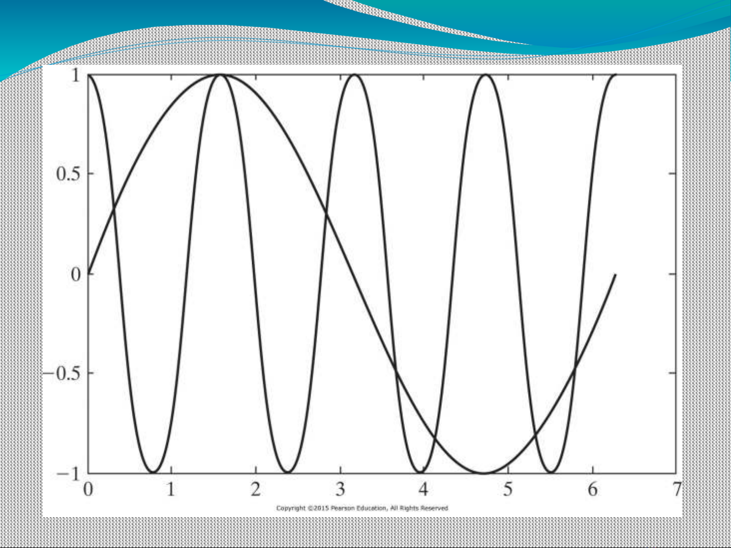
The hold on command can be used to layer plots on same graph
Continued…. Semicolons are optional on both the plot statement and the hold on statement MATLAB will continue to layer the plots until the hold off command is executed: hold off Another way to create a graph with multiple lines is to request both lines in a single plot command MATLAB interprets the input to plot as alternating x and y vectors, as in plot(X1, Y1, X2, Y2)
Continued…. If the plot function is called with a single matrix argument, MATLAB draws a separate line for each column of the matrix The x axis is labeled with the row index vector, 1: k , where k is the number of rows in the matrix. This produces an evenly spaced plot, sometimes called a line plot If plot is called with two arguments, one a vector and the other a matrix, MATLAB successively plots a line for each row in the matrix For example: we can combine y1 and y2 into a single
Continued…. Here’s another more complicated example: X = 0:pi/100:2*pi; Y1 = cos(X)*2; Y2 = cos(X)*3; Y3 = cos(X)*4; Y4 = cos(X)*5; Z = [Y1; Y2; Y3; Y4]; plot(X, Y1, X, Y2, X, Y3, X, Y4) This code produces the same result as
Multiple Plots on Same Graph
Continued…. A function of two variables, the peaks function produces sample data that are useful for demonstrating certain graphing functions Calling peaks with a single argument n will create an nxn matrix We can use peaks to demonstrate the power of using a matrix argument in the plot function The command plot(peaks(100)) results in the impressive graph
The peak Function, plotted with single augment in plot Command
Plots of Complex Arrays If the input to the plot command is a single array of complex numbers, MATLAB plots the real component on the x axis and the imaginary component on the y axis For example: if A = [0+0i,1+2i, 2+5i, 3+4i] then plot(A) title('Plot of a Single Complex Array') xlabel('Real Component')
Continued…. If we attempt to use two arrays of complex numbers in the plot function, the imaginary components are ignored The real portion of the first array is used for the x values, and the real portion of the second array is used for the y – values To illustrate, first create another array called B by taking the sine of the complex array A : B = sin(A) returns B = 0 3.1658 + 1.9596i 67.478930.8794i 3.8537 27.0168i
Line, Color and Mark Style The appearance of plots can be changed by selecting user defined line styles and line colors and by choosing to show the data points on the graph with user specified mark styles The command help plot returns a list of the available options
Continued…. The following commands illustrate the use of line, color, and mark styles: x = [1:10]; y = [58.5, 63.8, 64.2, 67.3, 71.5, 88.3, 90.1, 90.6, 89.5,90.4]; plot(x,y,':ok') The resulting plot (shown in next slide) consists of a dashed line, together with data points marked with circles
Continued…. To specify line, mark, and color styles for multiple lines, add a string containing the choices after each pair of data points If the string is not included, the defaults are used For example: plot(x,y,':ok',x,y*2,'xr',x,y/2,'b') results in the graph shown in next slide