Lecture note Data visualization - Chapter 29

Chia sẻ: Minh Nhật | Ngày: | Loại File: PPTX | Số trang:40

Thêm vào BST

Báo xấu

21
lượt xem 2
download

Download Vui lòng tải xuống để xem tài liệu đầy đủ

The main contents of the chapter consist of the following: The relational algebra, unary relational operations, relational algebra operations from set theory, binary relational operations, ER-to-Relational mapping algorithm, mapping EER model constructs to relations.

Chủ đề:

Bình luận(0) Đăng nhập để gửi bình luận!

Lưu

Nội dung Text: Lecture note Data visualization - Chapter 29

Lecture 29
Recap Summary of Chapter 6 Interpolation Linear Interpolation
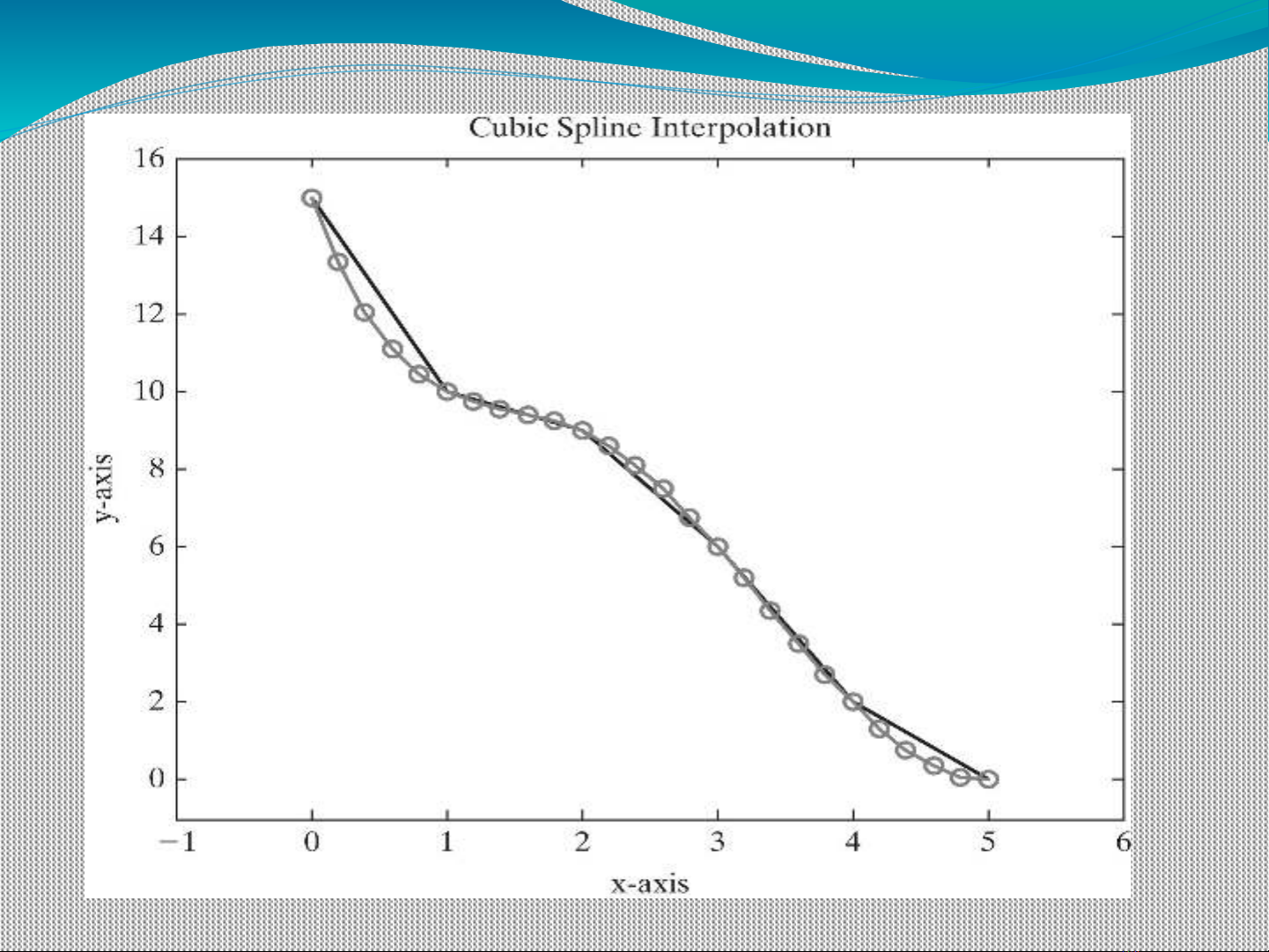
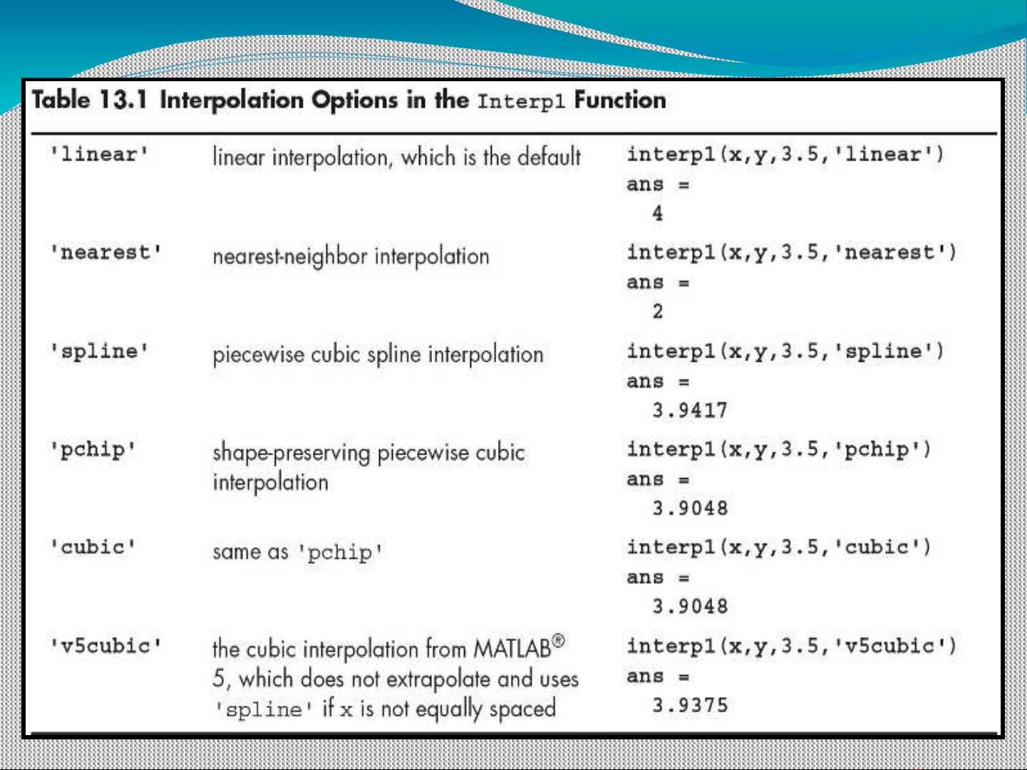
Cubic Spline Interpolation Connecting data points with straight lines probably isn’t the best way to estimate intermediate values, although it is surely the simplest A smoother curve can be created by using the cubic spline interpolation technique, included in the interp1 function. This approach uses a thirdorder polynomial to model the behavior of the data To call the cubic spline, we need to add a fourth field to interp1 : interp1(x,y,3.5,'spline') This command returns an improved estimate of y at x =
Multidimensional Interpolation Suppose there is a set of data z that depends on two variables, x and y . For example
Continued…. In order to determine the value of z at y = 3 and x = 1.5, two interpolations have to performed One approach would be to find the values of z at y = 3 and all the given x values by using interp1 and then do a second interpolation in new chart First let’s define x , y , and z in MATLAB : y = 2:2:6; x = 1:4; z = [ 7 15 22 30 54 109 164 218
Continued…. Although the previous approach works, performing the calculations in two steps is awkward MATLAB includes a twodimensional linear interpolation function, interp2 , that can solve the problem in a single step: interp2(x,y,z,1.5,3) ans = 46.2500 The first field in the interp2 function must be a vector defining the value associated with each column (in this case, x ), and the second field must be a vector defining
Continued…. MATLAB also includes a function, interp3 , for three dimensional interpolation Consult the help feature for the details on how to use this function and interpn , which allows you to perform n dimensional interpolation All these functions default to the linear interpolation technique but will accept any of the other techniques
Curve Fitting Although interpolation techniques can be used to find values of y between measured x values, it would be more convenient if we could model experimental data as y=f(x) Then we could just calculate any value of y we wanted If we know something about the underlying relationship between x and y , we may be able to determine an equation on the basis of those principles MATLAB has builtin curvefitting functions that allow us to model data empirically These models are good only in the region where we’ve collected data
Linear Regression The simplest way to model a set of data is as a straight line Suppose a data set x = 0:5; y = [15, 10, 9, 6, 2, 0]; If we plot the data, we can try to draw a straight line through the data
Continued…. Looking at the plot, there are several of the points appear to fall exactly on the line, but others are off by varying amounts In order to compare the quality of the fit of this line to other possible estimates, we find the
Continued….
Continued…. The linear regression technique uses an approach called least squares fit to compare how well different equations model the behavior of the data In this technique, the differences between the actual and calculated values are squared and added together. This has the advantage that positive and negative deviations don’t cancel each other out MATLAB could be used to calculate this parameter for data. We have sum_of_the_squares = sum((yy_calc).^2)
Continued…. Linear regression is accomplished in MATLAB with the polyfit function Three fields are required by polyfit : a vector of x –values a vector of y –values an integer indicating what order polynomial should be used to fit the data Since a straight line is a firstorder polynomial, enter the number 1 into the polyfit function: polyfit(x,y,1) ans = 2.9143 14.2857
Polynomial Regression
Continued…. We can find the sum of the squares to determine whether these models fit the data better: y2 = 0.0536*x.^23.182*x + 14.4643; sum((y2y).^2) ans = 3.2643 y3 = 0.0648*x.^3+0.5398*x.^24.0701*x + 14.6587 sum((y3y).^2) ans = 2.9921 The more terms we add to our equation, the “better” is the
Continued…. In order to plot the curves defined by these new equations, more than the six data points are used in the linear model MATLAB creates plots by connecting calculated points with straight lines, so if a smooth curve is needed, more points are required We can get more points and plot the curves with the following code: smooth_x = 0:0.2:5; smooth_y2 = 0.0536*smooth_x.^23.182*smooth_x +