Lecture note Data visualization - Chapter 30

Chia sẻ: Minh Nhật | Ngày: | Loại File: PPTX | Số trang:32

Thêm vào BST

Báo xấu

24
lượt xem 2
download

Download Vui lòng tải xuống để xem tài liệu đầy đủ

This chapter presents the following content: Cubic spline interpolation, multidimensional interpolation, curve fitting, linear regression, polynomial regression, the polyval function, the interactive fitting tools, basic curve fitting, curve fitting toolbox, numerical integration.

Chủ đề:

Bình luận(0) Đăng nhập để gửi bình luận!

Lưu

Nội dung Text: Lecture note Data visualization - Chapter 30

Lecture 30
Recap Cubic Spline Interpolation Multidimensional Interpolation Curve Fitting Linear Regression Polynomial Regression The Polyval Function The Interactive Fitting Tools Basic Curve Fitting Curve Fitting ToolBox
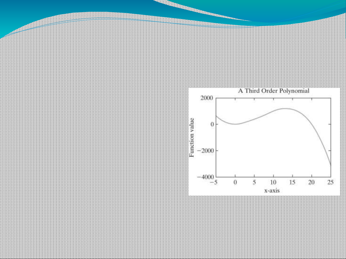
Numerical Integration Example Here’s another example, using a function handle and an anonymous function, instead of defining the function inside single quote First define an anonymous function for a thirdorder polynomial fun_handle = @(x)x.^3+20*x.^2 5 Now plot the function, to see how it behaves. The easiest approach is
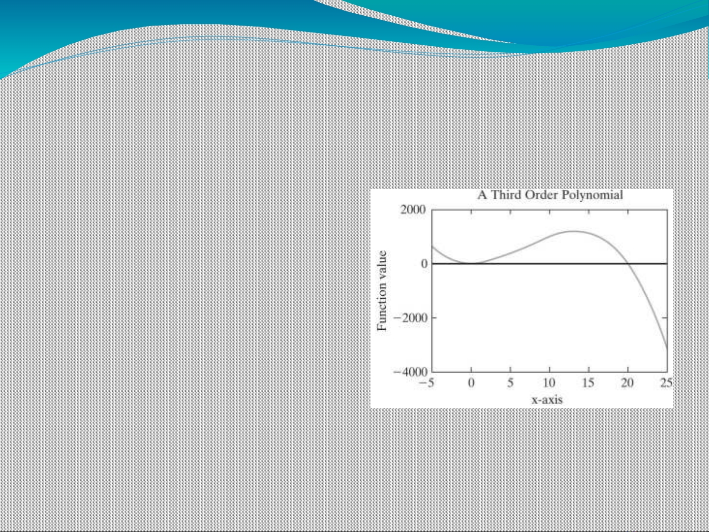
Example Continued….
Solving Differential Equation Numerically
Continued…. Each solver requires the following three inputs as a minimum: A function handle to a function that describes the fi rst order differential equation or system of differential equations in terms of t and y The time span of interest An initial condition for each equation in the system The solvers all return an array of t and y values: [t,y] = odesolver(function_handle,[initial_time, final_time], [initial_cond_array])
Function Handle Input
Continued….
Solving the Problem
Continued….
Continued…. When the input function or system of functions is stored in an Mfile, the syntax is slightly different The handle for an existing Mfile is defined as @m_file_name To solve the system of equations described in twofun we use the command ode45(@twofun,[1,1],[1,1]) The time span of interest is from 1 to 1, and the initial conditions are both 1
Solving HigherOrder Differential Equations
Continued…. Now all we need to do is create an Mfile function to use in one of the ode solvers The function should have two inputs, which are typically called t and y The variable t is the independent variable, and the variable y is an array of dependent variables In this example y (1) corresponds to the y used in the hand formulation, and y (2) corresponds to z The function containing the system of equations should look like this: function dydt = twoeq(t,y)
Continued…. Once the system of equations is defined in a function M file it is available to use as input to an ode solver For example: if the range of time is defined as 1 to +1 and the initial conditions are defined as y = 0 and z=0, then the command becomes ode45(@twoeq,[1,1],[0,0]) which gives the results A problem where the starting values are known is called an initial value problem
Boundary Value Problems bvp4c function is used to solve boundary value problems The bvp4c function requires three inputs: A function handle to the system of ode’s to be solved A function handle to a function that solves for the residual values of the function A set of guesses for the initial conditions
Continued…. The first function handle is exactly the same as we used for the ode solver set of functions It should contain the equations for the derivatives of interest and the results must be a column vector To solve the problem a guess is made for the initial value of all the derivatives, then the program checks to see how it did by comparing the calculated boundary values with the actual values For example, if: at t = 1, y = 0 and at t = 1, y = 3