EURASIP Journal on Applied Signal Processing 2005:18, 3076–3086 c(cid:1) 2005 C. Charoensak and F. Sattar
Design of Low-Cost FPGA Hardware for Real-time ICA-Based Blind Source Separation Algorithm
Charayaphan Charoensak School of Electrical and Electronic Engineering, Nanyang Technological University, Nanyang Avenue, Singapore 639798 Email: ecchara@ntu.edu.sg
Received 29 April 2004; Revised 7 January 2005
Blind source separation (BSS) of independent sources from their convolutive mixtures is a problem in many real-world multi- sensor applications. In this paper, we propose and implement an efficient FPGA hardware architecture for the realization of a real-time BSS. The architecture can be implemented using a low-cost FPGA (field programmable gate array). The architecture offers a good balance between hardware requirement (gate count and minimal clock speed) and separation performance. The FPGA design implements the modified Torkkola’s BSS algorithm for audio signals based on ICA (independent component analy- sis) technique. Here, the separation is performed by implementing noncausal filters, instead of the typical causal filters, within the feedback network. This reduces the required length of the unmixing filters as well as provides better separation and faster conver- gence. Description of the hardware as well as discussion of some issues regarding the practical hardware realization are presented. Results of various FPGA simulations as well as real-time testing of the final hardware design in real environment are given.
Farook Sattar School of Electrical and Electronic Engineering, Nanyang Technological University, Nanyang Avenue, Singapore 639798 Email: efsattar@ntu.edu.sg
Keywords and phrases: ICA, BSS, codesign, FPGA.
1. INTRODUCTION
time. Being fully custom-programmable, FPGA offers rapid hardware prototyping of DSP algorithms. The recent ad- vances in IC processing technology and innovations in the architecture have made FPGA a suitable alternative to using powerful but expensive computing platform.
Blind signal separation, or BSS, refers to performing inverse channel estimation despite having no knowledge about the true channel (or mixing filter) [1, 2, 3, 4, 5]. BSS technique has been found to be very useful in many real-world mul- tisensor applications such as blind equalization, fetal ECG detection, and hearing aid. BSS method based on ICA tech- nique has been found effective and thus commonly used [6, 7]. A limitation using ICA technique is the need for long unmixing filters in order to estimate inverse channels [1]. Here, we propose the use of noncausal filters [6] to shorten the filter length. In addition to that, using noncausal filters in the feedback network allows a good separation even in the case where the direct channels filters do not have stable in- verses. A variable step-size parameter for adaptation of the learning process is introduced here to provide a fast and sta- ble convergence. In spite of its potential for real-world applications, there have been very few published papers on real-time hardware implementation of the BSS algorithm. Many of the works such as [8] focus on the VLSI implementation and do not provide a detailed set of specifications of the BSS imple- mentation that offer a good balance between hardware re- quirement (gate count and minimal clock speed) and sepa- ration performance. Here, we propose an efficient hardware architecture that can be implemented using a low-cost FPGA and yet offers a good blind source separation performance. Extensive set of experimentations, discussion on separation performance, and the proposal for future improvement are presented.
This is an open access article distributed under the Creative Commons Attribution License, which permits unrestricted use, distribution, and reproduction in any medium, provided the original work is properly cited.
FPGA architecture allows optimal parallelism needed to handle the high computation load of BSS algorithm in real
The FPGA design process requires familiarity with the associated signal processing. Furthermore, the developed FPGA prototype needed to be verified, through both func- tional simulation and real-time testing, in order to fully un- derstand the advantages and pitfalls of the architecture under investigation. Thus, an integrated system-level environment
Maximize entropy
Adjust unmixing filter coefficients, W12 and W21
FPGA Hardware for Real-time ICA-Based BSS 3077
g(u)
g(u)
+
X1
W11
U1
W21
Mixed inputs
W12
Blind source separation output results
U2
+
X2
W22
Figure 1: Torkkola’s feedback network for BSS.
for software-hardware co-design and verification is need- ed. Here, we carried out FPGA design of a real-time implementation of the ICA-based BSS using a new system- level design tool called System Generator from Xilinx.
The rest of the paper is organized as follows. Section 2 provides an introduction to BSS algorithm and the appli- cation of noncausal filters within the feedback network. Section 3 describes the hardware architecture of our FPGA design for the ICA-based BSS algorithm. Some critical issues regarding the implementation of the BSS algorithm using the limited hardware resources in the FPGA are discussed. Section 4 presents the system level design of the FPGA fol- lowed by detailed FPGA simulation results, synthesis result, and the real-time experimentation of the final hardware us- ing real environment setup. The summary and the motiva- tions for future improvement are given in Section 5.
2. BACKGROUND OF BSS ALGORITHM
2.1. Infomax or entropy maximization criterion
M−1(cid:1)
quence, or a noncausal IIR filter. By truncating this non- causal IIR filter, the stable noncausal FIR filter (W12 or W21) can be realized [12]. It was also shown in [6] that the algo- rithm can be easily modified to use the noncausal unmix- ing FIR filters. The relationships between the signals are now changed to
k=−M
BSS is the main application of ICA, which aims at reducing the redundancy between source signals. Bell and Sejnowski [9] proposed an information-theoretic approach for BSS, which is referred to as the Infomax algorithm. (3) u1(t) = x1(t + M) + w12(k)u2(t − k),
M−1(cid:1)
2.2. Separation of convolutive mixture
k=−M
(4) u2(t) = x2(t + M) + w21(k)u1(t − k),
(cid:2)
(cid:2)
(cid:3)(cid:3) ,
(cid:2) ui
(cid:3) u j
(t1 −p1+M) = ∆wi j
(t0 −p0 +M) + K
where M is half of the filter length, L, that is, L = 2M + 1 and the learning rule The Infomax algorithm proposed by Bell and Sejnowski works well only with instantaneous mixture and was further extended by Torkkola for the convolutive mixture problem [10]. As shown in Figure 1, minimizing the mutual informa- tion between outputs u1 and u2 can be achieved by maximiz- ing the total entropy at the output. (5) ∆wi j t0 p0
(cid:3)(cid:3)
(cid:3)(cid:3)
L12(cid:1)
This architecture can be simplified by forcing W11 and W22 to be mere scaling coefficients to achieve the relation- ships shown below [6, 11]: where
(cid:2) = λ
(cid:2) t0
(cid:2) ui
(cid:3)
k=0
=
(cid:2) t0
(cid:2) t0 1 1 + e−ui(t0) ,
L21(cid:1)
, (6) K 1 − 2yi u1(t) = x1(t) + w12(k)u2(t − k), yi (1)
k=0
u2(t) = x2(t) + w21(k)u1(t − k), (7) for k = −M, −M + 1, . . ., M,
for k = −M, −M + 1, . . ., M. t1 = t0 + 1, p0 = t0 − k p1 = t1 − k and the learning rules for the separation matrix:
(cid:2) 1 − 2yi
(cid:3) u j(t − k).
The term λ in (6) represents the variable learning step (2) ∆wi j ∝ size which is explained in more detail in Section 3.5.
3. ARCHITECTURE OF HARDWARE 2.3. Modified ICA-based BSS method using modified FOR BSS ALGORITHM Torkkola’s feedback network
The top-level block diagram of our hardware architecture for the BSS algorithm based on Torkkola’s network is shown in Figure 2. The descriptions for the subsystems in the figure will be discussed in the following subsections. Some criti- cal issues regarding the practical realization of the algorithm while minimizing the hardware resources are discussed. Torkkola’s algorithm works only when the stable inverse of the direct channel filters exists. This is not always guaran- teed in real-world systems. Considering the acoustical condi- tion when the direct channel can be assumed a nonminimum phase FIR filter, the impulse response of its stable inverse will become noncausal infinite double-sided converging se-
Address for W
X1
U1
W12
Register
Entropy measurement
Unmixing filters W
Address for U
X2
MAC (muliply accumulate)
U2
U2
u1(t)
+
Address for X
Register
Variable learning stepping
Feedback network
Enable
X2 Memory blocks
Figure 2: Top-level block diagram of hardware architecture for BSS algorithm based on Torkkola’s network.
Figure 3: Implementation of (8) for the modified Tokkola’s feed- back network.
3078 EURASIP Journal on Applied Signal Processing
3.1. Practical implementation of the modified Torkkola’s network for FPGA realization
In order to understand the effect of each filter parameter such as filter length (L) and learning step size on the separation performance, a number of simulation programs written in MATLAB were tested. A set of compromised specification is then proposed for practical hardware realization [11].
needed to fill up a buffer. For example, if the signal sam- pling frequency is 8000 Hz, the time to fill up one buffer is 2500/8000 = 0.31 second. The system will then need another 0.31 second to process before the result being ready for out- put. The total delay is then 0.31 + 0.31 = 0.62 s. This process- ing delay may be too long for many real-time applications. A suggestion on applying overlapped processing windows, to- gether with polyphase filter, in order to shorten this delay is given in Section 5.
3.3. Implementation of feedback network mechanism As a result of our MATLAB simulations, we propose that in order to reduce the FPGA resource needed, as well as to ensure real-time BSS separation given the limited maximum FPGA clock speed, the specifications shown below are to be used. Sections 3.2 and 3.6 explain the impact of some param- eters on hardware requirement in more details.
M(cid:1)
i=−M
According to feedback network in (3), there is a need to ad- dress negative addresses for the values of w12(i) when i < 0. In practice, the equation is modified slightly to include only positive addresses: (i) Filter length, L = 161 taps. (ii) Buffer size for iterative convolution, N = 2500. (iii) Maximum number of iterations, I = 50. (iv) Approximation of the exponential learning step size using linear piecewise approximation. (8) u1(t) = x1(t + M) + w12(i + M)u2(t − i).
The linear piecewise approximation is used to avoid com- plex circuitry needed to implement the exponential func- tion (see Section 3.5 for more explanation of implementa- tion, and Section 4.2.1 for comparison of simulation results using exponential function and linear piecewise function). Equation (8) performs the same noncausal filtering on u2 as in (3) without the need for negative addressing of w12. Equation (4) is also modified accordingly.
There are many papers discussing the effect of filter length on the separation performance [13]. We have cho- sen a smaller filter length considering the maximum operat- ing speed of the FPGA and considered only the case of echo of a small room. (See Section 3.6 for calculation of required FPGA clock speed and Section 4.2.3 for the FPGA simulation result.) The block diagram shown in Figure 3 depicts the hard- ware implementation of (8). Note that the implementa- tion of the FIR filtering of w12 is done through multiply- accumulate unit (MAC) which significantly reduces the numbers of multipliers and adders needed when com- pared to direct parallel implementation. The tradeoff is that the FPGA has to operate at oversampling frequency (see Section 3.6). 3.2. Three-buffer technique
3.4. Mechanism for learning the filter coefficients The mechanism for learning of the filter coefficients was im- plemented according to (5). The implementation of the vari- able learning step size, λ, is explained in the next subsection.
3.5. Implementation of variable learning step size In order to speed up the learning of the filter coefficients shown in (5), we implement a simplified variable step-size technique. In real-time hardware implementation, to achieve an unin- terrupted processing, the hardware must process the input and output as streams of continuous sample. However, this is in contrast with the need of batch processing of BSS algo- rithm [14]. To perform the separation, a block of data buffer has to be filtered iteratively. Here, we implement a buffering mechanism using three 2500-sample (N = 2500) buffers per one input source. While one buffer is being filled with the in- put data, a second buffer is being filtered, and the third buffer is being streamed out.
A side effect of this three-buffer technique is that the sys- tem produces a processing delay equivalent to twice the time In our application, the variable learning step size in (6), that is, the learning step size λ, may be implemented using
FPGA Hardware for Real-time ICA-Based BSS 3079
(cid:4)
(cid:5) ,
(9) below where n is the iteration level, λ0 is the initial step size, and I is the maximum number of iterations, that is, 50:
− u0 − n I
(9) λ = exp
(cid:3)
where
(cid:2) λ0
− 1 I
(10) . u0 = − log2 Note that the frequency 64.4 MHz also represents the number of multiplications per second needed to perform the blind source separation (per channel). This represents a very large computation load if a general processor, or DSP (digital signal processor), is to be used for real-time applications. Us- ing fully hardware implementation, the performance gain is easily obtained by bypassing the fetch-decode-execute over- head, as well as by exploiting the inherent parallelism. FP- GAs allow the above-mentioned advantage plus the repro- grammability and cost effectiveness.
Some discussion on applying polyphase filter to increase the filter length while maintaining the FPGA clock speed is given in section 5.
4. SYSTEM-LEVEL DESIGN AND TESTING OF THE FPGA FOR BSS ALGORITHM
4.1. System-level design of FPGA for BSS algorithm The exponential term is difficult to implement in digi- tal hardware. Lookup table could be used but will require a large block of ROM (read only memory). Alternative to using lookup ROM is the CORDIC algorithm (COrdinate Rotation DIgital Computer) [15]. However, circuitry for CORDIC algorithm will impose a very long latency (if not heavily pipelined) which will result in the need for even higher FPGA clock speed. Instead, we used a linearly decreasing variable step size as shown:
for functional (11) λ = 0.0006 − 0.000012n.
System generator provides a bit-true and cycle-true FPGA blocksets simulation under MATLAB Simulink environment thus offering a very convenient and realistic system-level FPGA co-design and cosimulation. Some preliminary theoretical results from MATLAB m-file can directly be used as reference for verifying the FPGA results (refer to [16] and http://www.xilinx.com/system generator for more detailed description).
We had carried out MATLAB simulations to compare the separation performance using exponential equation and lin- ear piecewise term equation. It was found out that, using the specifications given in Section 3.1, there is no significant degradation in separation performance (see also simulation results in Section 4.2.1). A multipoint piecewise approxima- tion will be implemented in future improvement.
3.6. Calculation of the required FPGA clock speed
Note that the FPGA design using system generator is dif- ferent from the more typical approach using HDL (hardware description language) or schematics. Using system generator, the FPGA is designed by means of Simulink models. Thus, the FPGA functional simulation can be carried out easily right inside Simulink environment. After the successful sim- ulation, the synthesizable VHDL (VHSIC HDL where VH- SIC is very-high-speed integrated circuit) code is automati- cally generated from the models. As a result, one can define an abstract representation of a system-level design and easily transform it into a gate-level representation in FPGA. As mentioned earlier that in order to save hardware resource, multiply-accumulate (MAC) technique is used. This implies that MAC operation has to be done at a much higher rate than that of the input sampling frequency. This MAC operat- ing frequency is also the frequency of the FPGA clock. Thus, a detailed analysis of the FPGA system clock needed for real- time blind source separation is required.
The FPGA clock frequency can be calculated as shown in (12) (see also [11]) where Fs is the sampling frequency of the input signals, L is the tap length of the FIR filter, and I is the number of iterations:
(12) FPGA clock frequency = L · I · Fs. The top level design of the ICA-based BSS algorithm based on the described architecture is shown in Figure 4. As can be seen from the figure, the FPGA reads in the data from each wave file, and outputs the separated signals, as streams of 16-bit data sample. The whole design is made up of many subsystems. Here, a more detailed circuit design of the sub- system which implements the computation for updating the filter coefficients is shown in Figure 5.
In our FPGA design, filter tap L = 161, iterations I = 50, and input sampling frequency Fs = 8000 Hz; the FPGA clock frequency is thus
(13) 161 · 50 · 8000 = 64.4 MHz.
This means that the final FPGA design must operate properly at 64.4 MHz. In practice, the maximum operating speed of a hardware circuit can be optimized by analyzing the “critical path” in the design. A more detailed analysis of the critical path in the FPGA design is given in Section 4.1.2. The process of FPGA design is simplified. The Simulink design environment also enhances the system-level software- hardware co-design and verification. The upper right-hand side of Figure 3 shows how to use Simulink “scope” to dis- play the waveform generated by the FPGA during simula- tion. This technique can be used to display the waveform at any point in the FPGA circuitry. This offers a very prac- tical way to implement a software-hardware co-design and verification. Note also the use of the blockset “to wave file” to transfer the simulation outputs from the FPGA back to a wave file for further analysis.
Time scope
System generator
New u1
u1
Time scope 1
New u2
u2
try x1c.wav
To wave file
Input 1 Out 1
From wave file rss1 norm 1.wav (8000 Hz/1 Ch/16 b)
Input 2 Out 2
From wave file
try x2c.wav
Dbl Fpt Gateway in Dbl Fpt Gateway in
Fpt Dbl Gateway out Fpt Dbl Gateway out
To wave file 1
From wave file rss2 norm 1.wav (8000 Hz/1 Ch/16 b)
Terminator
Probe
T:[0 0], D:0
From wave file
Figure 4: Top-level design of BSS using system generator under MATLAB Simulink.
Addr
Addr muxa Sel D0 D1
Delay
3 Addr
And
Delay
Data Wa We
Wa
1 Out1
Sel D0 D1 Mem out mux
Delay
Sel D0 D1 Addr muxb
Addr
Data Wa
And
Delay
We
Wb
Figure 5: Detailed circuit for updating the filter coefficients.
3080 EURASIP Journal on Applied Signal Processing
4.1.1. Using fixed-point arithmetic in FPGA implementation
We use only fixed-point arithmetic in our design. As mentioned earlier, we use 16-bit fixed-point at the inputs and outputs of our FPGA design. In practice, depending on the applications, the size of data width should be selected taking into account the desired system performance and FPGA gate count. In terms of separation performance, it can be shown that word length of the accumulator unit in the MAC unit is most critical. Using system generator, it is easy to study the effect of round-off error on the overall system performance and that helps in selecting the optimal bit size in the final FPGA design.
When simulating a DSP algorithm using programming lan- guages such as C and MATLAB, double precision floating point numeric system is commonly used. In hardware im- plementation, fixed-point format numeric is more practical. Although several groups have implemented floating-point adders and multipliers using FPGA devices, very few practi- cal systems have been reported [17]. The main disadvantages of using floating point in FPGA hardware are higher resource requirements, higher clock frequency, and longer design time than an equivalent fixed-point system. 4.1.2. Analysis of critical path in FPGA implementation of BSS algorithm
For fixed filters, the analysis of the effect of fixed-point arithmetic on the filter performance has been well presented in other publications [18, 19]. An analysis of word length ef- fect on the adaptation of LMS algorithm is given in [18]. It was shown in Section 3.6 that in order for the FPGA to per- form the blind source separation in real time, the required
x
1 0.8 0.6
∗
+
Delay
MAC out
y
Figure 6: Simplified block diagram of MAC operation.
0.4 0.2 0 −0.2 −0.4 −0.6 −0.8 −1
0
1000
2000
3000
4000
5000
6000
7000
8000
(a)
FPGA Hardware for Real-time ICA-Based BSS 3081
clock frequency is 64.4 MHz. We will now analyze the criti- cal paths in the ICA-based BSS design in order to verify that the clock frequency can be met. Referring to Figures 1 and 2, one can see that the maximum operating speed of the FPGA is determined by the critical path in the multiply-accumulate blocks. The propagation delay in this critical path is the sum- mation of the combinational delay made up of one multiplier and one adder as shown in the simplified block diagram in Figure 6. Based on Xilinx data sheet of Virtex-E FPGA, de- lays of the dedicated pipeline multiplier and adder units are
1 0.8 0.6 0.4 0.2 0 −0.2 −0.4 −0.6 −0.8 −1
0
1000
2000
3000
4000
5000
6000
7000
8000
(b)
Figure 7: Two original female voices used for FPGA simulations: (a) first female voice and (b) second female voice.
(i) delay of 16-bits adder: 4.3 nanoseconds, (ii) delay of pipelined 16-bit multiplier: 6.3 nanoseconds.
Thus, we can approximate the total delays in the criti- cal path to be 4.3 + 6.3 = 10.6 nanoseconds, which converts to 94 MHz maximum FPGA clock frequency. This is much higher than the required 64.4 MHz needed. Note that this is only an approximation and we mention it here for the pur- pose of discussion about our BSS architecture. The accurate maximum clock speed can easily be extracted from the FPGA synthesis result which is given in Section 4.3. Note also that the available dedicated multipliers depend very much on the FPGA family and the size of device used.
4.2. Simulation results of the FPGA design for ICA-based BSS output, the voice is much more intelligible. Similar conclu- sion can be drawn for the other voice (the measurements to show the separation performance are given in the next sub- section).
We carried out experimentations using different wave files, all sampled at 8000 Hz, and with various types of mixing conditions. The output separation performance results were measured. The error of the separated first female voice, measured by subtracting the output in Figure 9a from the original input in Figure 7a, is shown in Figure 10a. Figure 10b shows error of the second voice.
4.2.1. FPGA simulation using two female voices In this simulation, we use wave files of two female voices. Each file is approximately one-second long, with sampling frequency of 8000 samples per second, and 16 bits per sam- ple. The files were preprocessed to remove dc component and amplitude normalized. The two original input voices are shown in Figures 7a and 7b, respectively.
Figures 11a and 11b show the FPGA simulation results using linear piecewise function, compared to exponential function shown in (7). Figure 11a shows the plot of learning step sizes, using exponential function and linear piecewise function, against number of iterations. Figure 11b compares the averaged changes of filter coefficients ∆w12 and ∆w21, for all the 161 taps, plotted against number of iterations. It can be seen that, for the maximum number of iterations used (= 50), both the learning step size using exponential func- tion and the learning step size using linear piecewise function converge to zeros properly. To simulate the mixing process, the two inputs were pro- cessed using the instantaneous mixing program called “in- stamix.m” downloaded from the website http://www.ele.tue. nl/ica99 given in [20]. The mixing matrix used is [0.6 1.0, 1.0 0.6]. The two mixed voices are shown in Figures 8a and 8b. 4.2.2. FPGA simulation using one female voice mixed with Gaussian noise
A second experiment was carried out to measure the sepa- ration performance of the FPGA under noisy environment [21]. The first female voice used in the last experimentation The separation results from the FPGA simulation are shown in Figures 9 and 10. The separated outputs are shown in Figures 9a and 9b. By comparing the separated out- put voice in Figure 9a to the corresponding mixed voice in Figure 8a, the separation is clearly visible. By listening to the
1 0.8
0.6
0.4 0.2
1 0.8 0.6 0.4 0.2 0 −0.2 −0.4 −0.6 −0.8 −1
0
1000
2000
3000
4000
5000
6000
7000
8000
0 −0.2 −0.4 −0.6 −0.8 −1
0
1000 2000 3000 4000 5000 6000 7000 8000 9000
(a)
(a)
1 0.8
1 0.8 0.6 0.4 0.2
0 −0.2 −0.4 −0.6 −0.8 −1
0
1000
2000
3000
4000
5000
6000
7000
8000
0.6 0.4 0.2 0 −0.2 −0.4 −0.6 −0.8 −1
0
1000 2000 3000 4000 5000 6000 7000 8000 9000
(b)
(b)
Figure 9: Two separated voices from FPGA simulation; (a) sepa- rated first voice and (b) separated second voice.
Figure 8: Two mixed female voices used for FPGA simulation. The program “instamix.m” downloaded from http://www.ele.tue.nl/ ica99 is used; (a) mixed first signal and (b) mixed second input.
3082 EURASIP Journal on Applied Signal Processing
(cid:8)
The improvement of SNR after BSS processing, SNRimp (dB), is defined as
2(i) 1(i)
(cid:6) (cid:7) T i=1 x2 (cid:7) T i=1 e2
SNRimp (dB) = 10 log (16) .
(cid:8)
(cid:6) (cid:7)
(cid:7)
was mixed with white Gaussian noise (see Figure 12) and the signal-to-noise ratios (SNRs), before and after the BSS opera- tion by the designed FPGA, were measured. The same mixing matrix [0.6 1.0, 1.0 0.6] was used. By adjusting the variance of the white Gaussian noise source, σ 2, the input SNR varies in the range −9 dB to 10 dB. The input signal-to-noise ratio, SNRi, is defined in this experimentation as
1(i) 2(i)
T i=1 x2 T i=1 x2
SNRi (dB) = 10 log (14) .
The result in Figure 13 shows the averaged output SNRs and the average improvement of SNRs plotted against input SNRs. It can be seen that as the input SNRs varies, the out- put SNRs is almost the constant at approximately 35 dB. The maximum achievable out SNRs is limited by the width of the datapath implemented inside the FPGA. Due to this reason, the amount of improvement of SNRs decreases with the in- creasing input SNRs.
Here, T is the total number of samples in the time period of measurement and x1(i) and x2(i) are the original female voice and the white Gaussian noise respectively. 4.2.3. FPGA simulation using two female voices mixed using simulated room environment
(cid:8)
Similarly, the output signal-to-noise ratio, SNRo, is de- fined in (15). e1(i) represents the overall noise left in the first separated output u1 and defined as e1(i) = u1(i) − x1(i) as shown in Figure 12:
1(i) 1(i)
(cid:6) (cid:7) T i=1 x2 (cid:7) T i=1 e2
SNRo (dB) = 10 log (15) . Next experimentation was carried out to measure separation performance of the designed FPGA under realistic room en- vironment using the same two female voices. The room envi- ronment was simulated using the program “simroommix.m” downloaded from the same website mentioned earlier. The coordinates (in meter) of the first and second signal sources
×10−3
e z i s p e t s
i
g n n r a e L
1 0.8 0.6 0.4 0.2 0 −0.2 −0.4 −0.6 −0.8 −1
1.8 1.6 1.4 1.2 1 0.8 0.6 0.4 0.2 0
0
1000 2000 3000 4000 5000 6000 7000 8000 9000
5
10
15
20
25
30
35
40
45
50
Iteration number
(a)
Exponential function Linear piecewise function
(a)
0.015
0.01
s e g n a h c
s t n e i c ffi e o c
1 0.8 0.6 0.4 0.2 0 −0.2 −0.4 −0.6 −0.8 −1
0.005
0
1000 2000 3000 4000 5000 6000 7000 8000 9000
e g a r e v A
r e t l fi f o
(b)
0
5
10
15
20
25
30
35
40
45
50
Iteration number
Figure 10: Error of the two separated voices; (a) error of separated first voice and (b) error of separated second voice.
Exponential function Linear piecewise function
(b)
FPGA Hardware for Real-time ICA-Based BSS 3083
Figure 11: (a) Learning step sizes using exponential and linear piecewise functions and (b) averaged changes of filter coefficients ∆w12 and ∆w21 using the two functions.
Delay
x1
u1
e1
−+ +
First female voice wave file
Mixing matrix
are (2, 2, 2) and (3, 4, 2) respectively. The locations of the first and second microphone are (3.5, 2, 2) and (4, 3, 2) respec- tively. The room size is 5 × 5 × 5. The simulated room ar- rangement is shown in Figure 14.
(cid:6)
(cid:8)
(cid:13)
(cid:12)(cid:2)
(cid:3)2
FPGA design of BSS algorithm
x2
u2
0.6 1.0 1.0 0.6
(cid:13)
.
(cid:3)2
i(cid:3)= j u j,xi
White Gaussian noise source with adjustable variance
Figure 12: FPGA simulation to test BSS using one female voice mixed with white Gaussian noise with adjustable variance σ 2.
The measurement of separation performance is based on using (17) (see [20]). Here, S j is the separation performance of the jth separated output where u j,x j is the jth output of the cascaded mixing/unmixing system when only input x j is active; E[u] represents the expected value of u: u j,x j E (cid:12)(cid:2) (cid:7) (17) S j = 10 log E
The program “bsep.m,” which performs the computation as shown in (17), was downloaded from the website and used to test our FPGA. It was found that before the BSS,
(18) S1 = 17.29 dB, S2 = 10.63 dB,
and after the BSS operation, improvement can be made by increasing the filter lengths. Note also that the measurements of separation performance and the improvement after the BSS depend very much on the room arrangement. (19) S1 = 20.29 dB, S2 = 16.53 dB. 4.2.4. FPGA simulation using convolutive mixture of voices
In order to test the FPGA using convolutive mixtures recorded in a real cocktail party effect, two samples voices were downloaded from a website (T-W Lee’s website Thus, the BSS hardware improves the separation by 3 dB and 5.9 dB for channels 1 and 2, respectively. The figures may not appear very high. However, by listening to the separated output signals, the improvement was obvious and further
45
Table 1: Detailed gate requirement of the BSS FPGA design.
40
35
s R N S t u p t u O
30
s R N S f o t n e m e v o r p m
i d n a
Number of slices for logic Number of slices for flip flops Number of 4 input LUTs used as LUTs used as a route-thru used as shift registers Total equivalent gate count for the design
550 405 3002 2030 450 522 100 213
25
−8
−6
−4
−2
0
2
4
6
8
20 −10
Table 2: Maximum combinational path delay and operating fre- quency of the FPGA design for BSS.
Input SNRs (dB)
Output SNRs Improvement of SNRs after BSS
Maximum path delay from/to any node Maximum operating frequency
15.8 ns 71.2 MHz
Figure 13: Results of SNR measurements using one female voice mixed with white Gaussian noise. The figure shows the output SNRs and the improvement of SNRs against the input SNRs.
3084 EURASIP Journal on Applied Signal Processing
surement of the separation performance. However, by listen- ing to the separated outputs, we notice approximately the same level of separation as in our earlier experimentations.
5
4
)
3
Voice 2
Microphone 2
2
Microphone 1
m 5 ( t h g i e H
1
Voice 1
0 5
4
L
e
3
5
n
4.3. FPGA synthesis result
4
2
gth (
5
3
m
1
)
2
1
0
0
After the successful simulation, the VHDL codes were auto- matically generated from the design using system generator. The VHDL codes were then synthesized using Xilinx ISE 5.2i and targeted for Virtex-E, 600 000 gates. The optimization setting for the ISE is for maximum clock speed. Table 1 de- tails the gate requirement of the FPGA design. The total gate requirement reported by the ISE is approximately 100 kgates. The price of the FPGA device in this range of gate size is very low. Note that all of the buffers are implemented using exter- nal memory. Table 2 shows the reported maximum path delay and the highest FPGA clock frequency.
W i d t h ( 5 m )
Figure 14: Arrangement of female voice sources and microphones in simulated room environment using program “simroommix.m.”
4.4. Real-time testing of FPGA design
The real-time testing of the FPGA was done using a proto- type board equipped with a 600 000-gate Virtex-E FPGA de- vice. The system setup is shown in Figure 15. The wave files of the convolutive mixtures used in Section 4.2.4 were encoded into the left and right channels of a stereo MP3 file which is then played back repeatedly using a portable MP3 player. The prototype board is equipped with 20-bit A/D and D/A con- verters and the sampling frequency was set to 8000 samples per second. Only the highest 16 bits of the sampled signals were used by the FPGA.
The FPGA streamed out the separated outputs which were then converted into analog signals, amplified, and played back on the speaker. By listening to the playback sound, it was concluded that we had achieved the same level of separation as found in earlier simulations.
5. SUMMARY
at http://inc2.ucsd.edu/∼tewon/) and used in the FPGA simulation. The two wave files used were from two speak- ers recorded speaking simultaneously. Speaker 1 counts the digits from one to ten in English and speaker 2 counts in Spanish. The recording was done in a nor- mal office room. The distance between the speakers and the microphones was about 60 cm in a square ordering. A commercial program was used to resample the original sampling rate of 16 kHz down to 8000 Hz. The separation re- sults from the developed FPGA can be found at our website (http://www.ntu.edu.sg/home/ecchara/—click project on the left frame). Note that we present a real-time experimentation using these convolutive mixtures in Section 4.4. We have also posted the separation results of the same convolutive mix- tures using MATLAB program at the same website for com- parison.
In this paper, the hardware implementation of the modi- fied BSS algorithm was realized using FPGA. A set of com- promised specification for the BSS algorithm was proposed Because the original wave files (before the convolutive mixing) were not available, we could not perform the mea-
Figure 15: System setup for real-time testing of the blind source separation in real time.
FPGA Hardware for Real-time ICA-Based BSS 3085
In this paper, we consider the case of 2 sources (or 2 voices) and 2 sensors (or 2 microphones). In the future, we will carry out further improvements in our FPGA archi- tecture to tackle the situation when the number of sources is higher, or lower, than the number of sensors. Using our existing design, we have done some FPGA simulation us- ing 3 voices with 2 microphones. The separation results are good (please visit the website http://www.ntu.edu.sg/home/ ecchara/ for listening test). In this situation, two of the three voices are successfully separated (from each other) while the third suppressed voice is still present at both of the outputs. We will improve on our current FPGA design to handle this situation. Considering the fact that redesigning the FPGA takes much time, we will carry out the above improvements in our future works.
[1] T.-W. Lee, Independent Component Analysis: Theory and Ap- plications, Kluwer Academic, Hingham, Mass, USA, 1998. [2] R. M. Gray, Entropy and Information Theory, Springer, New
York, NY, USA, 1990.
REFERENCES
[3] P. Comon, “Independent component analysis, a new con- cept?” Signal Processing, vol. 36, no. 3, pp. 287–314, 1994. [4] K. Torkkola, “Blind source separation for audio signals—are we there yet?” in Proc. IEEE International Workshop on Inde- pendent Component Analysis and Blind Signal Separation (ICA ’99), pp. 239–244, Aussois, France, January 1999.
[5] T.-W. Lee, A. J. Bell, and R. Orglmeister, “Blind source sepa- ration of real world signals,” in Proc. IEEE International Con- ference on Neural Networks (ICNN ’97), vol. 4, pp. 2129–2134, Houston, Tex, USA, June 1997.
taking into consideration the separation performance and hardware resource requirements. The design implements the modified Torkkola’s BSS algorithm using noncausal unmix- ing filters which reduce filter length and provides faster con- vergence. There is no whitening process of the separated sources involved except that there is a scaling applied in the mixed inputs proportional to their variances.
[6] F. Sattar, M. Y. Siyal, L. C. Wee, and L. C. Yen, “Blind source separation of audio signals using improved ICA method,” in Proc. 11th IEEE Signal Processing Workshop on Statistical Signal Processing (SSP ’01), pp. 452–455, Singapore, August 2001. [7] H. H. Szu, I. Kopriva, and A. Persin, “Independent compo- nent analysis approach to resolve the multi-source limitation of the nutating rising-sun reticle based optical trackers,” Op- tics Communications, vol. 176, no. 1-3, pp. 77–89, 2000. [8] C. Abdullah, S. Milutin, and C. Gert, “Mixed-signal real-time adaptive blind source separation,” in Proc. International Sym- posium on Circuits and Systems (ISCAS ’04), pp. 760–763, Van- couver, Canada, May 2004.
[9] A. J. Bell and T. J. Sejnowski, “An information-maximisation approach to blind separation and blind deconvolution,” Neu- ral Computation, vol. 7, no. 6, pp. 1129–1159, 1995.
[10] K. Torkkola, “Blind separation of convolved sources based on information maximization,” in Proc. IEEE Signal Processing Society Workshop on Neural Networks for Signal Processing VI, pp. 423–432, Kyoto, Japan, September 1996.
The FPGA design was carried out using a system level approach and the final hardware achieves the real-time oper- ation using minimal FPGA resource. Many FPGA functional simulations were carried out to verify and measure the sepa- ration performance of the proposed simplified architecture. The test input signals used include additive mixtures, convo- lutive mixtures, and simulated room environment. The re- sults show that the method is robust against noise; that is, producing a small variation of the output SNR with respect to a large variation in the input SNR. Note that here we have considered the sensors to be almost perfect, or high quality with negligible sensor error.
[11] F. Sattar and C. Charayaphan, “Low-cost design and imple- mentation of an ICA-based blind source separation algo- rithm,” in Proc. 15th Annual IEEE International ASIC/SOC Conference (ASIC/SOC ’02), pp. 15–19, Rochester, NY, USA, September 2002.
[12] B. Yin, P. C. W. Sommen, and P. He, “Exploiting acoustic similarity of propagating paths for audio signal separation,” EURASIP Journal on Applied Signal Processing, vol. 2003, no. 11, pp. 1091–1109, 2003.
[13] H. Sawada, S. Araki, R. Mukai, and S. Makino, “Blind source separation with different sensor spacing and filter length for each frequency range,” in Proc. 12th IEEE Workshop on Neural
A relatively short filter length of 161 tap is first attempted here due to the limitation of the maximum clock speed of the FPGA. The FPGA can perform the separation successfully when the delay is small, that is, less than 161/8000 = 20 ms. In the environment where the delay is longer, a much longer filter tap is needed and this can be realized. In this case, we propose that, in order to keep the FPGA clock frequency the same, multiple MAC engines should be used together with the implementation of polyphase decomposition. For exam- ple, if the tap length of 161 ∗ 16 = 2576 is needed, 16 MACs engines are to be implemented with the 16-band polyphase decomposition. Since one MAC engine is made up of only one multiplier and one accumulator, the additional MAC en- gines will not lead to much additional gates.
The application of block mode separation leads to the side effect of a long processing delay. It was shown in Section 3.2 that our current design poses a long delay of 0.62 s. A practical solution to this long delay is to apply over- lapped processing windows. For example, if the processing delay is to be reduced to 0.62/32 = 20 ms, the 2500-sample windows will have to be overlapped by 31/32 = 97%, that is, the BSS has to be performed for every 78 input samples.
Networks for Signal Processing (NNSP ’02), pp. 465–474, Mar- tigny, Valais, Switzerland, September 2002.
[14] A. Cichocki and A. K. Barros, “Robust batch algorithm for se- quential blind extraction of noisy biomedical signals,” in Proc. 5th International Symposium on Signal Processing and Its Ap- plications (ISSPA ’99), vol. 1, pp. 363–366, Brisbane, Queens- land, Australia, August 1999.
[15] R. Andraka, “A survey of CORDIC algorithms for FPGAs,” in Proc. ACM/SIGDA 6th International Symposium on Field Pro- grammable Gate Arrays (FPGA ’98), pp. 191–200, Monterey, Calif, USA, February 1998.
[16] Xilinx, Xilinx System Generator v2.3 for the MathWorks
Simulink: Quick Start Guide, February 2002.
[17] J. Allan and W. Luk, “Parameterised floating-point arithmetic on FPGAs,” in Proc. IEEE International Conference on Acous- tics, Speech, and Signal Processing (ICASSP ’01), vol. 2, pp. 897–900, Salt Lake City, Utah, USA, 2001.
[18] J. R. Treichler, C. R. Johnson Jr., and M. G. Larimore, The- ory and Design of Adaptive Filters, Prentice-Hall, Upper Saddle River, NJ, USA, 2001.
[19] S. Haykin, Adaptive Filter Theory, Prentice-Hall, Upper Saddle
River, NJ, USA, 1996.
[20] D. Schobben, K. Torkkola, and P. Smaragdis, “Evaluation of blind signal separation methods,” in Proc. IEEE International Workshop on Independent Component Analysis and Blind Sig- nal Separation (ICA ’99), pp. 261–266, Aussois, France, Jan- uary 1999.
[21] A. K. Barros and N. Ohnishi, “Heart instantaneous frequency (HIF): an alternative approach to extract heart rate variabil- ity,” IEEE Trans. Biomed. Eng., vol. 48, no. 8, pp. 850–855, 2001.
3086 EURASIP Journal on Applied Signal Processing