
REGULAR ARTICLE
Statistical model of global uranium resources and long-term
availability
Antoine Monnet
1*
, Sophie Gabriel
1
, and Jacques Percebois
2
1
French Alternative Energies and Atomic Energy Commission, I-tésé, CEA/DEN, Université Paris Saclay, 91191 Gif-sur-Yvette,
France
2
Université Montpellier 1–UFR d’Économie–CREDEN (Art-Dev UMR CNRS 5281), Avenue Raymond Dugrand, CS 79606,
34960 Montpellier, France
Received: 25 September 2015 / Received in final form: 5 January 2016 / Accepted: 19 January 2016
Published online: 8 April 2016
Abstract. Most recent studies on the long-term supply of uranium make simplistic assumptions on the available
resources and their production costs. Some consider the whole uranium quantities in the Earth’s crust and then
estimate the production costs based on the ore grade only, disregarding the size of ore bodies and the mining
techniques. Other studies consider the resources reported by countries for a given cost category, disregarding
undiscovered or unreported quantities. In both cases, the resource estimations are sorted following a cost merit
order. In this paper, we describe a methodology based on “geological environments”. It provides a more detailed
resource estimation and it is more flexible regarding cost modelling. The global uranium resource estimation
introduced in this paper results from the sum of independent resource estimations from different geological
environments. A geological environment is defined by its own geographical boundaries, resource dispersion
(average grade and size of ore bodies and their variance), and cost function. With this definition, uranium
resources are considered within ore bodies. The deposit breakdown of resources is modelled using a bivariate
statistical approach where size and grade are the two random variables. This makes resource estimates possible
for individual projects. Adding up all geological environments provides a repartition of all Earth’s crust resources
in which ore bodies are sorted by size and grade. This subset-based estimation is convenient to model specific cost
structures.
1 Long-term cumulative supply curves
(LTCS)
The availability of natural uranium will have a direct
impact on the global capability to build new nuclear
reactors in the coming decades as it is forecasted that Light
Water Reactors (LWRs) will remain the main nuclear
technology for most of the 21st century [1,2]. The cost
associated with this availability is also important. Even
though its share in the electricity production cost is
relatively low, it may influence the choice of fuel cycle
options in the short term or the choice of reactor
technologies in the long term.
1.1 Concepts and objectives
Considering natural uranium as any other mineral commodi-
ty, academics in mineral economics and decision makers in
mining industries usually look at availability by the mean of
two analytical tools. The first one is generally called cash-cost
curve. This curve consists in plotting the cumulated
production capacity (tU/year) of all known production
capacities, either running mines or short-term projects,
against the unit production cost ($/kgU) of those mines once
they have been sorted by cost merit order. This tool essentially
helps analyzing short-term to medium-term availability
issues, i.e. from a couple of years to a decade or two.
Since the objective of this research is to analyze the
adequacy of uranium supply to long-term demand, another
tool was preferred as it suits availability problems with
implications over several decades. This tool is the long-term
cumulative supply curve (LTCS). It was made popular by
Tilton et al. [3,4] in 1987. The curve depicts the cumulated
amount (tU) of all known resources, eventually adding
estimates of undiscovered resources, after they have been
* e-mail: antoine.monnet@cea.fr
EPJ Nuclear Sci. Technol. 2, 17 (2016)
©A. Monnet et al., published by EDP Sciences, 2016
DOI: 10.1051/epjn/e2016-50058-x
Nuclear
Sciences
& Technologies
Available online at:
http://www.epj-n.org
This is an Open Access article distributed under the terms of the Creative Commons Attribution License (http://creativecommons.org/licenses/by/4.0),
which permits unrestricted use, distribution, and reproduction in any medium, provided the original work is properly cited.
sorted by rising unit production cost ($/kgU). Unlike cash-
cost curve, there is no time dimension in the LTCS curve. In
order to assess the adequacy of supply to demand over time,
one would need to compare the LTCS curve with a time-
dependent demand scenario. In this paper, the stress is put
on the method used to build the LTCS curve.
1.2 Aggregated LTCS curve
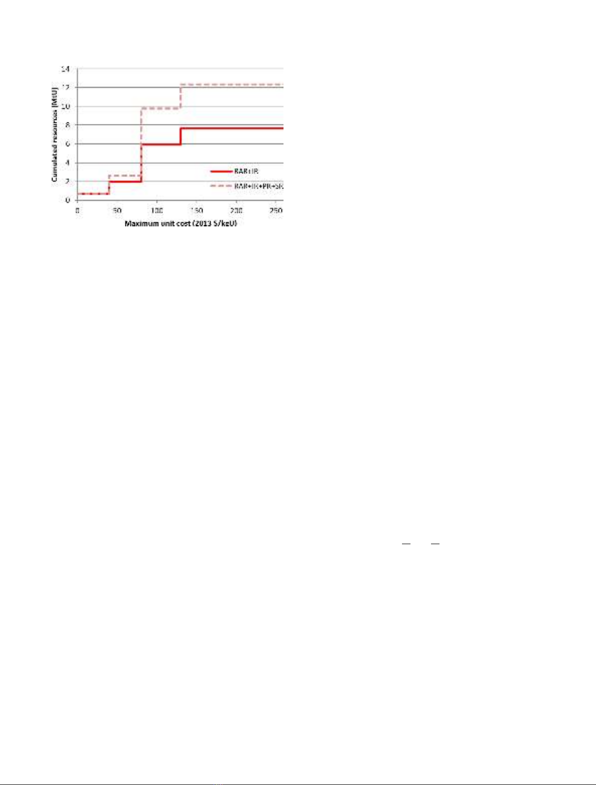
The easiest way to build a LTCS curve is to aggregate
existing data of cumulated resources and associated
production costs published in the literature or in technical
reports. Focusing on uranium, this can be achieved by
gathering the resources declared by countries in the IAEA/
OECD-NEA biennial report called the Red Book [5]. The
result is shown in Figure 1 for the aggregation of total
known resources (Reasonably Assured Resources [RAR]
and Inferred Resources [IR], red curve, and for total known
and prognosticated resources [RAR + IR + Prognosticated
Resources (PR) + Speculative Resources (SR)], light-red
curve).
1.3 Limits of the aggregation approach
The aggregation approach to build LTCS curves is
convenient provided that consistent data are available.
Conversely, it can be criticized due to the aggregation of
different levels of uncertainty in the example of the Red
Book data. By definition, the amount and the cost of
prognosticated or speculative resources are more uncertain
than known resources (RAR or IR) to which they were
added in the light-red curve (Fig. 1). While the analysis is
usually performed by assuming that cheaper resources are
extracted first, there is no guarantee that undiscovered
resources between 40 and 80 $/kgU will all be discovered
before RAR at below 80 $/kgU are exhausted. Conversely,
if one only considers known resources (red curve, Fig. 1), it
is likely that some resources at below 80 $/kgU that are not
known at present will be discovered in the long term.
Finally, using aggregated data to perform analysis on
LTCS curves has two limits. First, when data are
incomplete, long-term resources are underestimated. Sec-
ond, when data are over-aggregated, short-term resources
may be overestimated while the long-term is affected by a
growing uncertainty on costs. This appears on the upper
part of the light-red curve for which 3 MtU of SR are
missing since they have no cost estimate reported in the Red
Book. These limits prompted some academics to develop
alternative methods to build LTCS curve.
2 Global elastic crustal abundance models
To avoid aggregating estimates with different cost and
amount uncertainties, some recent studies, mainly con-
ducted by Schneider from University of Texas and
Matthews and Driscoll from MIT [6–8], model the costs
and quantities of resources of the entire Earth’s crust with
the same methodology. They introduce a 3-step method to
build LTCS curves:
–first, they model the link between the quantity
(cumulated amount) and the quality (represented by
ore grade) of resources;
–second, they model the link between the unit production
cost and the quality of resources;
–finally, they infer from the first two steps the general
relation between cumulated amounts of resources and
associated costs.
From this framework, the elastic crustal abundance
model provides a LTCS curve for the entire world.
2.1 Step 1: quantity-quality relationship
The authors introduce a power relationship between
the grade gand the cumulated amount of metal qaccording
to equation (1). This results in an elastic relationship in log-
scale where ais the elasticity of quantities in relation to
grades and where q
0
and g
0
are calibration parameters.
q
q0
¼g0
g
a
:ð1Þ
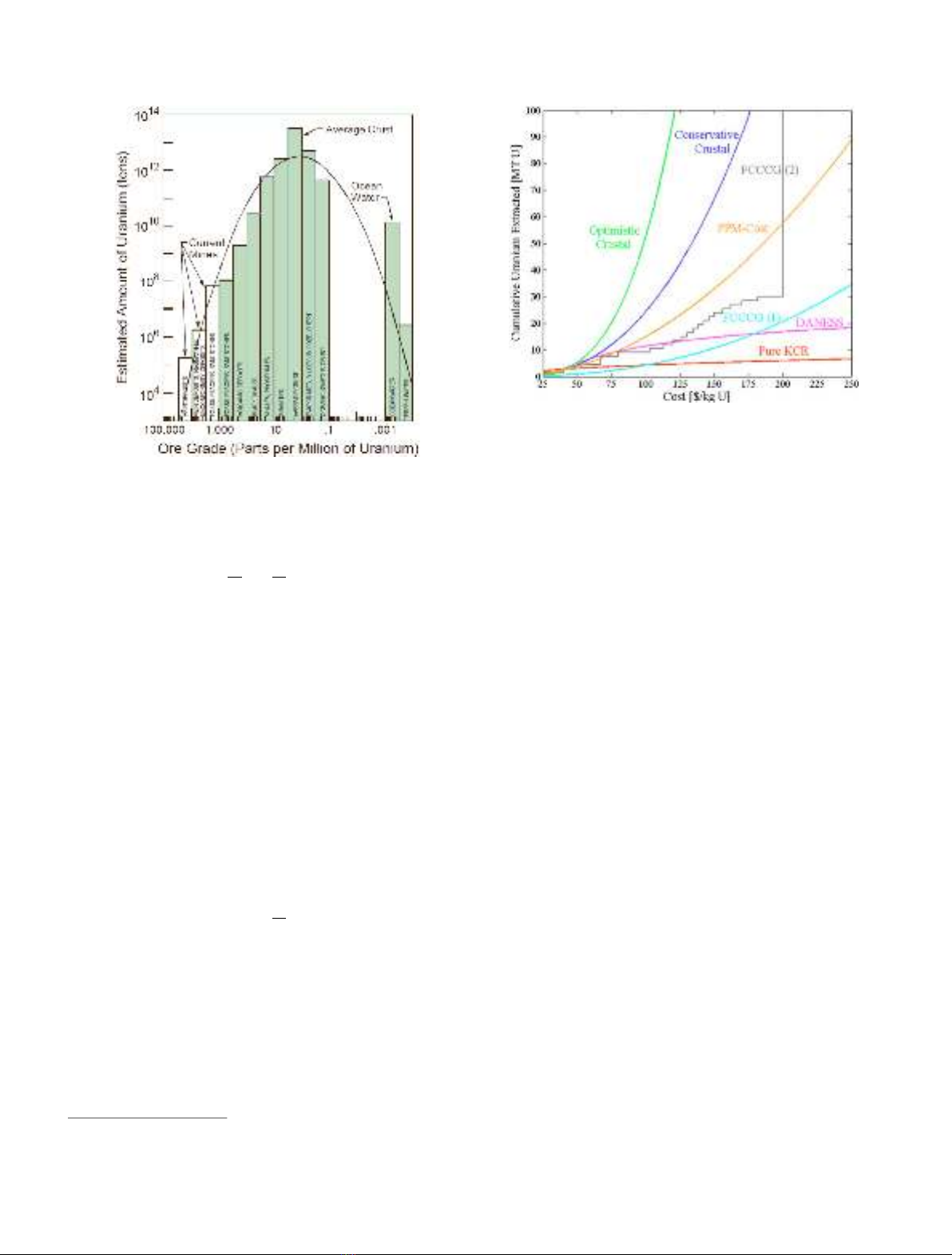
As explained in the MIT study [8], an empirical rela-
tionship between cumulated uranium resources and ore
grades is used to estimate a. This empirical relationship was
established in 1979 by Deffeyes and Macgregor [9]. It is a well-
known bell-shape relationship, as depicted in Figure 2.In
the high-grade range (10
2
–10
4
ppmU), the bell-shape curve
is approximated by its slope denoted by ain equation (1).
2.2 Step 2: cost-quality relationship
The second relationship (Eq. (2)) introduced by the authors
is also a power-relation. This time, brepresents the
elasticity of unit costs in relation to grades; g
0
and c
0
are
calibration parameters.
Fig. 1. Long-term supply curve built from the 2014 Red Book
data [5].
2 A. Monnet et al.: EPJ Nuclear Sci. Technol. 2, 17 (2016)
g
g0
¼c0
c
b:ð2Þ
Different versions of this relationship can be found in
the literature. While Schneider makes the simple assump-
tion that b= 1 before looking at sensitivity, the MIT study
introduces a more complex expression of bto take account
of learning effects in addition to economies of scale. Finally,
different versions of the relationship can be found depend-
ing on the value of b, either imposed or fitted. A number of
them are gathered in Schneider and Sailor paper [6].
2.3 Step 3: cost-quantity model
Once the previous two relations are defined, step 3 derives
the cost-quantity relationship from equations (1) and (2),
according to equation (3).
q¼q0
c
c0
ab
:ð3Þ
In this formula, the product denoted by ab can be
interpreted as the global elasticity of supply to unit costs of
production. The LTCS curve is finally obtained by plotting
the relationship of equation (3), once all parameters have
been fitted or calibrated. Figure 3 shows the LTCS curves
presented by Schneider for different versions of the previous
framework
1
.
2.4 Limits of the elastic crustal abundance models
At this stage, several shortcomings can be raised against the
framework proposed by Schneider, Matthews and Driscoll.
First, the results are sensitive to calibration (Sect. 2.4.1).
Second, only one intrinsic parameter of the resource, i.e. its
grade, is used to determine both the geological availability
(Eq. (1))(Sect. 2.4.2) and the economic value of the
resource (Eq. (2))(Sect. 2.4.3).
2.4.1 Sensitivity to calibration (Eq. (3))
The final equation (Eq. (3)) for the LTCS curve requires a
calibration point denoted by (q
0
,c
0
). Although Schneider
investigates the sensitivity of ab through different versions
of his model (Fig. 3), the sensitivity to calibration is not
covered. This paper conducts this sensitivity analysis
according to the following methodology.
The cumulative resources (q
0
) and the corresponding
cost limits (c
0
) were taken from various editions of the Red
Book. To run the following sensitivity tests, the version of
the elastic crustal abundance model that was used is
Schneider’s‘optimistic crustal’model (ab = 3.32). Table 1
presents the different calibration points that were consid-
ered and Figure 4 shows the resulting sensitivity.
Figure 4 shows how the choice of the calibration points
affects the LTCS curve.
2.4.2 Limits to quantity-grade relationship (Eq. (1))
In the late 1970s, Deffeyes and Macgregor [9] reported
imperfections in the bell-shape distribution of the grades.
They noted that in the case of chromium, but also uranium,
certain high grades can be overrepresented compared to the
theoretical model, as shown in Figure 5.
Deffeyes explained this kind of bimodal distribution
by particular forms of mineralization. These would be
formed by a different sequence of independent phenomena
Fig. 3. Long-term cumulative supply curves for different versions
of the elastic crustal abundance model [6].
Fig. 2. Empirical bell-shape relationship between cumulated
uranium resources and ore grades [9].
1
To be more correct, FCCCG(2) and DANESS models differ from
the elastic crustal abundance model. These specific characteristics
are not covered by this paper.
A. Monnet et al.: EPJ Nuclear Sci. Technol. 2, 17 (2016) 3
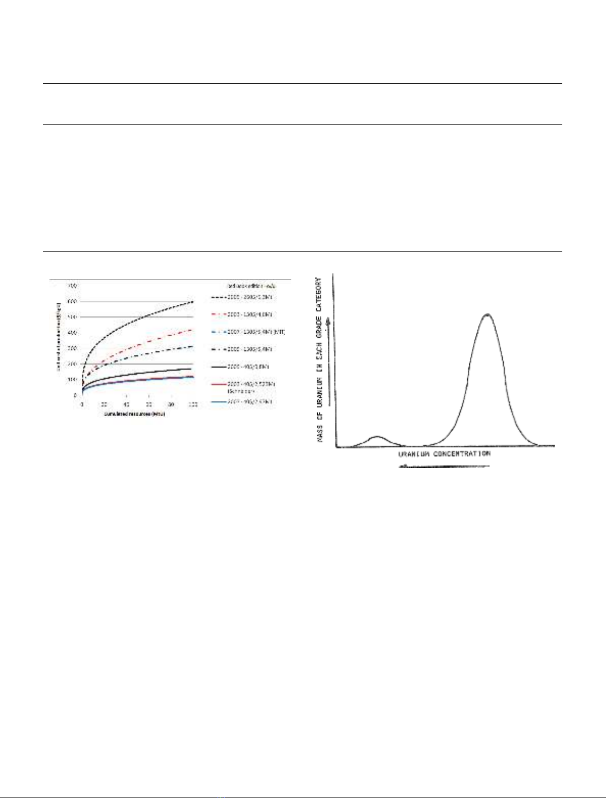
compared to the sequence of the main distribution and
result in a separate distribution. This point is important
since it was shortly after Deffeyes’publications that the
main very high-grade deposits of Saskatchewan in Canada
were discovered (Cigar Lake in 1981, McArthur River in
1988). The inclusion of these deposits in the diagram of
Figure 2 invalidates the bell-shape model used in
Schneider’s and Matthews’methods.
2.4.3 Limits to the cost-grade relationship (Eq. (2))
Apart from scale effects, considering the unit cost of
production as only a function of grade can be opened to
criticism. Today, some running uranium mines, which must
have similar total production costs to be competitive in the
current market, have substantially different grades [10]:
–Cigar Lake, Canada (underground, 14.4% U, $23/lb
U
3
O
8
nominal operating cost);
–South Inkai, Kazakhstan (in situ leaching, 0.01% U, $22/
lb U
3
O
8
nominal operating cost).
Conversely, some projects of similar grades may have
quite different production costs [10]. In the following
example, the production cost for in situ leaching is mainly
operating cost, whereas for open pit, capital costs cannot be
omitted:
–Carley Bore, Australia (in situ leaching, 0.03% U,
$20/lb U
3
O
8
nominal operating cost);
–Letlhakane, Botswana (open pit, 0.02% U, $58/lb U
3
O
8
nominal operating cost).
As a consequence of the limits of the two previous
relationships, the outputs of the model are not robust: as
suggested in Figure 3, different values for the elasticity
parameters ab can change the output significantly and
no acceptable conclusion on available resources can be
found.
While grade is certainly an important factor in the cost of
a resource, there are other parameters that govern cost and it
may be desirable to model them. These include the size of ore
bodies and the geochemical nature of deposits. Any change in
these parameters can lead to specific mining techniques and
therefore specific costs. When a deposit is located in a given
country with specific legislation, taxes and royalties can also
be taken into account through the cost.
Table 1. Calibration points (c
0
,q
0
).
Red Book edition RAR
(MtU)
Identified
(RAR + IR)
(MtU)
Identified + Undiscovered
(RAR + IR + SR + PR)
(MtU)
2003 3.2 <130 $/kgU 2.523 <40 $/kgU
(Schneider’s ref.)
4.6 <130 $/kgU
14.4
2007 3.3 <130 $/kgU 2.97 <40 $/kgU
4.5 <80 $/kgU
5.4 <130 $/kgU
(MIT ref. for Identified)
15.9
(MIT ref. for Identified + Undiscovered)
2009 4.0 <260 $/kgU 0.8 <40 $/kgU
3.7 <80 $/kgU
5.4 <130 $/kgU
6.3 <260 $/kgU
16.7
Fig. 4. Sensitivity of the elastic crustal abundance model in
relation to calibration points.
Fig. 5. Bimodal relationship between cumulated uranium
resources and ore grades [9].
4 A. Monnet et al.: EPJ Nuclear Sci. Technol. 2, 17 (2016)

Thus, if the cost function keeps a limited number of
parameters, it can be more realistic to calibrate each deposit
category or geological environment individually (one
calibration for Canadian underground mines, one calibra-
tion for Australian ISL mines, etc.).
3 A statistical approach based on geological
environments
To overcome the limits of previous models, this paper
proposes a statistical approach that differs on three points
from the elastic crustal abundance models:
–geological availability and production costs are estimated
by a bivariate model. The two variables are grade (mean
grade of a deposit, denoted g) and tonnage (ore tonnage of
a deposit, denoted t);
–the scope of the model is split to several regional crustal
abundance estimations. These regions are called geologi-
cal environments
2
. A geological environment is defined by
its own geographical boundaries, resource dispersion
(average grade and size of ore bodies and their variance),
and cost function;
–a statistical approach is adopted. Variables gand tare
treated as random variables and their probability density
functions (pdfs) serve to build the corresponding
relationship.
Section 3.1 briefly presents former geostatistical models,
which have been applied to uranium endowment and share
the same framework as the one developed in this article. Then
Sections 3.2 to 3.4 describe the methodology step-by-step.
3.1 Former geostatistical models
Several bivariate or multi-variate statistical models for
crustal abundance and associated costs can be found in
the literature. Their objectives are the same as in Section 2
but rather than proceeding to the economic appraisal of
cumulative quantities, statistical models proceed to the
economic appraisal at a deposit level and then add up
all the resources of deposits. The benefit of this approach
is that models can be specific to each geological
environment.
Among the models available in the literature, three have
been applied to uranium endowment estimation. They were
developed by Drew [11], Harris et al. [12–15] and Brinck
[16–18]. None of them served to build a complete LTCS
curve (rather they served to estimate the undiscovered
resources at below a given cost, i.e. the price of U
3
O
8
at the
time of the studies), but some parts inspired the model
developed in this paper. The general framework can be
described in three parts which differ a little from the three
steps described in Section 2 :
–For a specific environment, the geological abundance q
can be defined using a constant q
0
, the total metal
endowment of the geological environment, and a
probability density function f(g,t) (Eq. (4)):
q¼q0∫∫ fg;tðÞdgdt:ð4Þ
q
0
is estimated from the mass of rock Min the geological
environment and the mean grade of the crust (clarke)
(q
0
=Mclarke). It should be noticed that this q
0
has no
embedded consideration about economics nor technical
recovery, unlike the calibration values used in Section 2.3.
qis derived from the statistics of gand tamong the
known deposits of a given geological environment. Since
these statistics are biased (high-grade and high-tonnage
deposits tend to be first discovered), a specific method is
required to derive the unbiased function f(g,t). This method
is based on economic filtering.
–The second part consists in a cost model which is similar
to that of elastic crustal abundance models, except costs
are estimated at a deposit level and ore tonnage is taken
into account. The resulting cost-grade-tonnage relation-
ship is of the form described by equation (5), which can be
also written as in equation (6) with x=ln(g),y=ln(t)
and Aa constant.
cg;t
ðÞ
¼c0
g
g0
bgt
t0
bt
ð5Þ
ln cg;tðÞðÞA¼bgxþbty:ð6Þ
–In part 3, Drew proposes to compute the cumulated metal
resources available at below a given unit production cost
C
1
by using to intermediate calculations: the numerical
computation of N, the total number of deposits in the
environment (the total mass of rock Mdivided by the
mean tonnage of all deposits), and m(C
1
), the mean metal
content of deposits that are “cheaper than C
1
”. Equations
(7) and (8) give the analytical expressions of Nand m(C
1
)
in terms of statistical expectations.
N¼M
∫∫ ∞
0tf g;tðÞdgdt ð7Þ
mC
1
ðÞ¼ ∬
cg;tðÞC1
gtf g;tðÞdgdt:ð8Þ
Finally, the LTCS curve is built by plotting the function
C
1
→Nm(C
1
).
2
This terminology was first used in Drew [11]. It is convenient
because the model produces an assessment of geological resources
rather than reserves within the environment. Yet, the meaning of
“geological”can be confusing. The boundaries do not aim to circle a
single geological structure but rather groups of structures that
share a maximum of common properties (types, size, grade of
known deposits and also economic, political conditions) compared
with other environments (e.g. US groups of deposits vs. Canada,
Australia, Africa or Kazakhstan).
A. Monnet et al.: EPJ Nuclear Sci. Technol. 2, 17 (2016) 5


![Ngân hàng trắc nghiệm Kỹ thuật lạnh ứng dụng: Đề cương [chuẩn nhất]](https://cdn.tailieu.vn/images/document/thumbnail/2025/20251007/kimphuong1001/135x160/25391759827353.jpg)