
121
5
DISCRETE IMAGE MATHEMATICAL
CHARACTERIZATION
Chapter 1 presented a mathematical characterization of continuous image fields.
This chapter develops a vector-space algebra formalism for representing discrete
image fields from a deterministic and statistical viewpoint. Appendix 1 presents a
summary of vector-space algebra concepts.
5.1. VECTOR-SPACE IMAGE REPRESENTATION
In Chapter 1 a generalized continuous image function F(x, y, t) was selected to
represent the luminance, tristimulus value, or some other appropriate measure of a
physical imaging system. Image sampling techniques, discussed in Chapter 4,
indicated means by which a discrete array F(j, k) could be extracted from the contin-
uous image field at some time instant over some rectangular area ,
. It is often helpful to regard this sampled image array as a
element matrix
(5.1-1)
for where the indices of the sampled array are reindexed for consistency
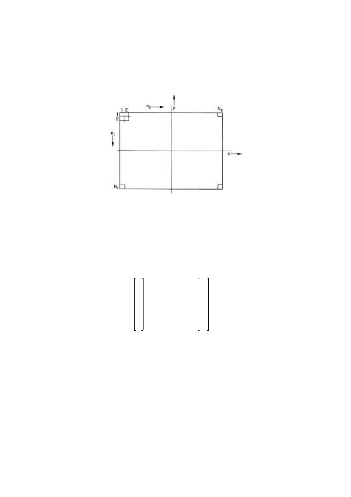
with standard vector-space notation. Figure 5.1-1 illustrates the geometric relation-
ship between the Cartesian coordinate system of a continuous image and its array of
samples. Each image sample is called a pixel.
J–jJ≤≤
K–kK≤≤ N1N2
×
FFn
1n2
,()[]=
1niNi
≤≤
Digital Image Processing: PIKS Inside, Third Edition. William K. Pratt
Copyright © 2001 John Wiley & Sons, Inc.
ISBNs: 0-471-37407-5 (Hardback); 0-471-22132-5 (Electronic)
122 DISCRETE IMAGE MATHEMATICAL CHARACTERIZATION
For purposes of analysis, it is often convenient to convert the image matrix to
vector form by column (or row) scanning F, and then stringing the elements together
in a long vector (1). An equivalent scanning operation can be expressed in quantita-
tive form by the use of a operational vector and a matrix
defined as
(5.1-2)
Then the vector representation of the image matrix F is given by the stacking opera-
tion
(5.1-3)
In essence, the vector extracts the nth column from F and the matrix places
this column into the nth segment of the vector f. Thus, f contains the column-
FIGURE 5.1-1. Geometric relationship between a continuous image and its array of
samples.
N21×vnN1N2
⋅N2
×Nn
vn
0
0
1
0
0
=
…
…
1
n1–
n
n1+
N2
……
Nn
0
0
1
0
0
=
……
1
n1–
n
n1+
N2
……
fN
nFvn
n1
=
N2
∑
=
vnNn

GENERALIZED TWO-DIMENSIONAL LINEAR OPERATOR 123
scanned elements of F. The inverse relation of casting the vector f into matrix form
is obtained from
(5.1-4)
With the matrix-to-vector operator of Eq. 5.1-3 and the vector-to-matrix operator of
Eq. 5.1-4, it is now possible easily to convert between vector and matrix representa-
tions of a two-dimensional array. The advantages of dealing with images in vector
form are a more compact notation and the ability to apply results derived previously
for one-dimensional signal processing applications. It should be recognized that Eqs
5.1-3 and 5.1-4 represent more than a lexicographic ordering between an array and a
vector; these equations define mathematical operators that may be manipulated ana-
lytically. Numerous examples of the applications of the stacking operators are given
in subsequent sections.
5.2. GENERALIZED TWO-DIMENSIONAL LINEAR OPERATOR
A large class of image processing operations are linear in nature; an output image
field is formed from linear combinations of pixels of an input image field. Such
operations include superposition, convolution, unitary transformation, and discrete
linear filtering.
Consider the element input image array . A generalized linear
operation on this image field results in a output image array as
defined by
(5.2-1)
where the operator kernel represents a weighting constant, which,
in general, is a function of both input and output image coordinates (1).
For the analysis of linear image processing operations, it is convenient to adopt
the vector-space formulation developed in Section 5.1. Thus, let the input image
array be represented as matrix F or alternatively, as a vector f obtained by
column scanning F. Similarly, let the output image array be represented
by the matrix P or the column-scanned vector p. For notational simplicity, in the
subsequent discussions, the input and output image arrays are assumed to be square
and of dimensions and , respectively. Now, let T
denote the matrix performing a linear transformation on the input
image vector f yielding the output image vector
(5.2-2)
FN
n
Tfvn
T
n1
=
N2
∑
=
N1N2
×Fn
1n2
,()
M1M2
×Pm
1m2
,()
Pm
1m2
,() Fn
1n2
,()On
1n2m1m2
,;,()
n21
=
N2
∑
n11
=
N1
∑
=
On
1n2m1m2
,;,()
Fn
1n2
,()
Pm
1m2
,()
N1N2N== M1M2M==
M2N2
×N21×
M21×
pTf=

124 DISCRETE IMAGE MATHEMATICAL CHARACTERIZATION
The matrix T may be partitioned into submatrices and written as
(5.2-3)
From Eq. 5.1-3, it is possible to relate the output image vector p to the input image
matrix F by the equation
(5.2-4)
Furthermore, from Eq. 5.1-4, the output image matrix P is related to the input image
vector p by
(5.2-5)
Combining the above yields the relation between the input and output image matri-
ces,
(5.2-6)
where it is observed that the operators and simply extract the partition
from T. Hence
(5.2-7)
If the linear transformation is separable such that T may be expressed in the
direct product form
(5.2-8)
MN×Tmn
T
T11 T12 …
……
…T1N
T21 T22 …
……
…T2N
TM1TM2…TMN
=
…
…
…
pTN
nFvn
n1
=
N
∑
=
PM
m
Tpum
T
m1
=
M
∑
=
PM
m
TTNn
()Fv
num
T
()
n1
=
N
∑
m1
=
M
∑
=
MmNnTmn
PT
mnFv
num
T
()
n1
=
N
∑
m1
=
M
∑
=
TT
CTR
⊗=
GENERALIZED TWO-DIMENSIONAL LINEAR OPERATOR 125
where and are row and column operators on F, then
(5.2-9)
As a consequence,
(5.2-10)
Hence the output image matrix P can be produced by sequential row and column
operations.
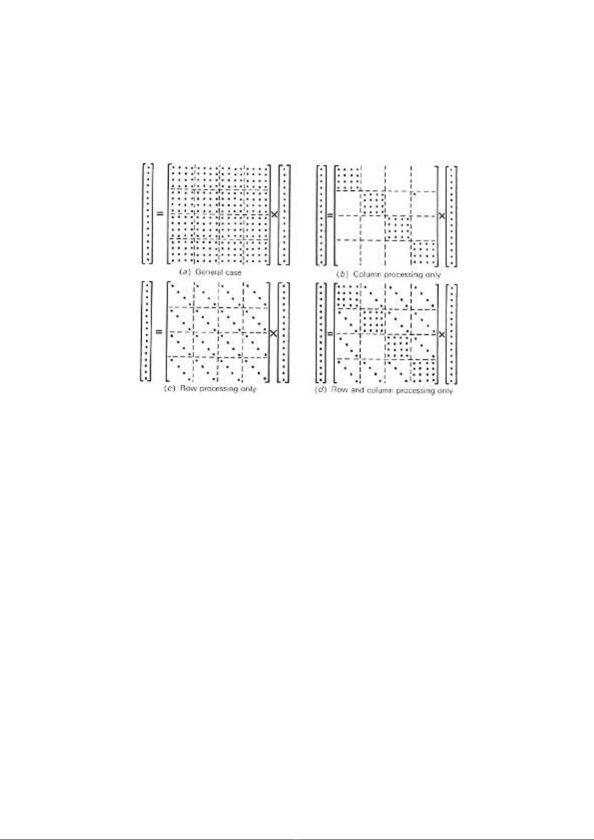
In many image processing applications, the linear transformations operator T is
highly structured, and computational simplifications are possible. Special cases of
interest are listed below and illustrated in Figure 5.2-1 for the case in which the
input and output images are of the same dimension, .
FIGURE 5.2-1. Structure of linear operator matrices.
TRTC
Tmn TRmn,()TC
=
PT
CFTRmn,()vnum
T
n1
=
N
∑
m1
=
M
∑TCFTR
T
==
MN=


![Sổ tay Kỹ thuật cơ điện [chuẩn nhất]](https://cdn.tailieu.vn/images/document/thumbnail/2026/20260520/vispacex_27/135x160/2321779253898.jpg)


![Giáo trình Trang bị điện cơ bản (Nghề Điện công nghiệp TC) - Trường Cao đẳng Kỹ thuật Đồng Nai [Mới nhất]](https://cdn.tailieu.vn/images/document/thumbnail/2025/20251212/laphong0906/135x160/58031779074467.jpg)


![Giáo trình Trang bị điện nước (TC) - Trường Cao đẳng Công nghiệp Thanh Hóa [Ngành Điện nước]](https://cdn.tailieu.vn/images/document/thumbnail/2026/20260511/hoatrami2026/135x160/14221778681890.jpg)


