Practice 1: Introduction to the ArcView Interface and the
Data
Terms to know .................................................................................................................. 1
ArcView Steps .................................................................................................................. 1
Step 1 Start ArcView .................................................................................................... 1
Step 2 Add a New View to the Project ......................................................................... 2
Step 4 Set the Working Directory ................................................................................ 3
Step 5 Create the Project ............................................................................................ 3
Step 6 Add a Theme to the View ................................................................................. 3
Step 7 Turn on the Themes and arrange the draw order ............................................ 4
Step 8 Change the theme symbology ......................................................................... 4
Step 9 Give the Themes and View meaningful names ............................................... 4
Step 10 Zooming in and out ........................................................................................ 5
Step 11 Change the way we see the Europe .............................................................. 5
Step 12 Locating Sheffield (or your area) on the Globe .............................................. 6
In this first practice, you will learn a few important fundamentals about ArcView's graphical
user interface (GUI) as well as how to locate yourself on a map. In this first practice you will also
become familiar with some of the data that you will be using in later practices. Getting familiar
with your data is an important beginning step when using a GIS. These fundamentals will help
you be more efficient during the next practices in this project.
In this practice you will leam how to open ArcView (version 3.2), start a new project, add a
view, and set the working directory (where you save the files that you create). You will also leam
how to add themes to a view, turn them on, arrange an appropriate draw order, and change the
symbols. In this practice you will take time to get familiar with many of the menus, buttons, and
tools that you will use in the next practices. Also, from the next practice, you will also leam how to
open an attribute table and perform a simple query. Last, but not least, in this practice you will
leam about map coordinates, scale and changing map projections.
Terms to know
• Shapefile: a file storage unit that ArcView uses.
• Theme: the type of data you are looking at. For example, roads, rivers, soil, mountain
peaks, or wildemess areas. Each theme will be either a point, line, or polygon shape.
Think of it as a "theme of a party!" (The theme ofmy 'point' party is 'mountain peaks').
• Attribute: characteristics about a theme that are contained in a table. Every theme has an attribute table. • Query: when you select a portion of a theme based on an attribute in the table you are making a query. You are asking the table or the spatial data a question. • Coordinates: locations on the surface of earth where a feature is located. Measured in latitude and longitude or decimal degrees. • Feature: one or more features make a theme, for example, one road in the roads theme is a feature. • Projection: a perspective of the surface of the earth that will distort the shape, area, distance, or direction of the features in a theme.
• Scale: the units on the ground as compared to the units on the map. For example, a scale
of 1:25,000 means that 1 unit on the map equals 25,000 units on the ground. The unit is
usually a measure of distance (i.e. inches, feet, miles, meters, or kilometers).
ArcView Steps
Step 1 Start ArcView
To access ArcView from the university server, you need to download ArcView package
internally in your computer. The below picture illustrates the procedure to access Arc View: Select
Start and then, Application, Academic, Social Science, and finally ArcView GIS .
Practice 2: Working with tables
ArcView Steps .................................................................................................................. 8
Step 1 Opening data .................................................................................................... 8
Step 2 Table properties ............................................................................................... 9
Step 3 Adding data to the table ................................................................................... 9
Step 4 Simple table functionality ............................................................................... 10
Step 5 Selecting features........................................................................................... 10
Step 6 The query builder ........................................................................................... 10
Step 7 Creating new tables ....................................................................................... 11
Step 8 Joining tables ................................................................................................. 11
In this practical you will discover how to open, edit, create and
work with tables. Firstly, you will need to start ArcView, start a new
project, add a view and set the working directory (to 'c:\') as
demonstrated in the last practice. An ArcView project can contain
any number oftables - to see which tables are in a project click onthe
tables' icon in the 'project window'.
ArcView Steps
Step 1 Opening data
Click the Add Theme button. Navigate to the directory for
'c:\arcv32\arcview\esridata\usa'. Select the following theme:-
'states.shp'. Click OK. This theme will now be added to your view. We are going to edit data within the theme and do
not want to overwrite the original file and so we will have to make a copy ofthe data. Make sure
the 'states' theme is active by clicking on the theme in the legend (the area will appear raised or
3-D). Go to the 'Theme' menu and select 'Convert to Shapeflle' - as illustrated below:-
Call the converted theme 'States' and save it to you u directory. We no longer require the
Practice 2: Working with tables ERS 120: Principles of GIS
original data - so make the theme active, then go to the 'Edit' menu and select 'Cut Theme.'. Now make the new 'States' theme active and then click on the 'Open Theme Table' button (
). You should now see all the attribute information relevant for the states theme. Each record
(row) represents one state and each field (column) is a variable containing information
appertaining to the states. You can use the scroll bars to either scroll down or up to see more
records, or scroll right and left to examine the various fields.
Step 2 Table properties
We are now going to change the table name and edit the fields that are visibl e to us speeding
up display of the table within ArcVi ew. Go to the 'Table' menu and select 'Properties'. We can
rename the title of the table - let's call it 'American States'. Next, in the visible column click to
uncheck all apart from the following: Shape; Area; State name; Pop1990; PopI1997; and Pop90
sqmi. Don't click on the OK just yet.
All the other fields will now no longer appear in the table display - although they have NOT
been deleted from the database- we just can't see them. Find the field called 'Pop90 sqmi' within
the table properties dialog box. Click in the 'Alia.' column next to this entry and type 'Population
density 1990'. -Then click OK for your changes to take effect. The field name we changed is now too long to fit within the display
properly. We can ext end the size of the field by moving the mouse
over the edge of the field name and by clicking and holding the left-
mouse button (see figure below), then move the mouse to extend the
fields visible area. We can also re-arrange the order of the fields. Click on the name
at the top of the column and drag it right or left. This doesn't re-
arrange the table itself-just how we see it within ArcView. Experiment by changing the order of
the fields.
Step 3 Adding data to the table
Firstly, we have to start editing the table, go to the 'Table' menu and select 'Start Editing'. To
add a field, go to the 'Edit' menu and select 'Add Field'. Type the name of the attribute - in this
case 'Pop change'
Under 'Type' you can choose the type of data you will be entering: 'Number' for numerical
entries; 'String' for text (word) information; or 'Boolean' for true/false entries. We are entering
numbers for this field. The 'width' corresponds to the number of characters that can fit within the
field, for example 'xxxx' occupies 4 character spaces.
Indicate the number of decimal places required - we do not require them so leave it as the
default of '0'. Click 'OK' - you should now see your new column added to the right side of the
table.
Click on the 'Edit' button ( ).We are now ready to enter data into the table. We could do it manually by hand but there are 51 records in this table (shown in the top left hand side
) and so an automated data entry would be much quicker.
Make sure the field title (pop_change) is highlighted - it should appear a darker grey than the
other field titles), then click on the
'Calculate' button (
). This will
allow us to write an equation that
ArcView will solve and enter into
the column. We require population change
and so double click on the
following; 'Pop1999' from the
fields list; '-' from the requests;
and then on the field 'Pop 1990',
Your display should now resemble
the figure below. Click on 'OK' to
start the calculations. After a few
seconds you should see the
results fill the 'Pop_change'
N.D. Bình 9/59
Practice 2: Working with tables ERS 120: Principles of GIS
column. Once finished choose 'Stop Editing' from the table menu and save your edits.
Step 4 Simple table functionality
We can sort each field either in ascending or descending order using the following buttons (
). The find record button ( ) can be used to find the first record whose data items
contain the input character/numeric string. For example try searching for 'New York' to find the
appropriate record.
Step 5 Selecting features
• a) Select button - use this button to commence 'selection mode'
• b) Edit button - click on this to be enable edit mode to input into the table
• c) Identify - used to view record fields within vertical viewing box
You can select records in the table to work with them. Sort the 'Population_change' field by
descending order. Click on California's record (remember you must be in selection mode using
the 'Select Button' illustrated at the top of the page) – notice that it is now highlighted yellow - this
means the record is selected. If you now look within 'View1' (you may have to minimise the table),
the geographical state of California will also be highlighted yellow. We can select multiple records
within the table by holding down the 'shift' key while clicking on records. Selecting records can also work the other way round - by selecting states within the view,
corresponding records in the table will be highlighted. Click on the 'Select Feature' tool (
),and
then click on a state within the view - the record will now be highlighted within the table. Multiple
records can be selected by holding the mouse button when using the 'select feature' tool. Select
the states of Alaska and Hawaii (see below) and return to the table.
The selected features may
not necessarily be visible, so to
move the selected records to the
top of the table click on the
). If you 'Promote' button (
now click on the 'Switch
Selection' button (
) the
highlighted records will be
unselected and those that were
previously selected will now be
highlighted. To select all the records within the table use the 'Select All' button (
). When you
have finished examining the possible ways of selecting records, choose the 'Select None' button (
) to deselect all records.
Step 6 The query builder
Feature selection can also be accomplished using an SQL (Structured Query Language)
) or
expression using the database fields and values. Click on the 'Query Builder' button (
select 'Query' from within the 'Theme' menu. Double click on the field to query; then single click
an operator; and double click on either a value or manually type the required criteria.
Options within the 'query builder' include:
lists and updates all unique values in the chosen field
New selection set - features not m the set are unselected
Adds features to existing selected set > Update values:
> New set:
> Add to set:
> Select from set: Selects from existing selected set
Use the query builder to select all the states that have suffered a decrease in the population
N.D. Bình 10/59
Practice 2: Working with tables ERS 120: Principles of GIS
between 1990 and 1997. You can also build a character string query by using double quotations
and wildcards (*), for example:
Find all states that begin with the letter A
( [Statename1= "A*")
Find all states that contain the letter A
( [Statename1= "*A*")
Remember to click on the 'New Set' button to create a new selection or 'Add to set' to add this
new query to a previous query selection. Experiment using the two different options (for example
select all states beginning with "A" using a new set, and then add all stat es beginning with "N"). Try these examples and think of some for yourself. Once you have finished experimenting with
to clear selected the query builder and the use of wildcards - use the 'Select None' button
features from both the database (table) and graphical (the VIew) displays.
Step 7 Creating new tables
To create a table from scratch - click on the 'new' button within the 'project window ' and create a new table called 'cities' in your c directory.
Once the blank table has opened click on 'Add Field' within the 'Edit ' menu. Repeat to create the following fields:
Now go to the 'Edit ' menu and select 'Add Record'. Repeat this to enter the following
information (note ArcView is case-sensitive so us e capital1etters exactly as shown below):
Step 8 Joining tables
You can join a second table to the active table, based on the values of a common field found
in both table s. Joins establish a one-to-one, or many-to-one relationship between the destination
N.D. Bình 11/59
Practice 2: Working with tables ERS 120: Principles of GIS
table (the active table) and the source table (the tab le you are joining into the active table).
Typically, the source table contains descriptive attributes of features that you wish to join into a
themes table so that you can symbolise, label, query and analyse the features in the theme using
the data from your source table.
Joins can be accomplished using any data type (String, Number, Boolean or Date).
We are now going to join the ' states' and ' cities' tables. Open the ' states' table and then click
on the 'State _name' field header (see figure 1 below), then open the ' cities' table and select the
) is no longer
'State_name' field header (see figure 2). Note how now the 'Join' button (
greyed out - click on it. If the 'Join' button is not available then it is most likely because one of the
tables is still being edited. The two table s should now be joined - as illustrated within figure 3
below.
Notice how the relevant 'states' attributes have now been added to the 'cities' table. The tables
have not been physically linked and the results are only visible in this form within ArcView. To
save the new table it either has to be exported and re-imported; or add new fields and use the
'calculator' to input the information. To return the table to its previous form select 'Remove All
Joins' from the 'Table' menu. You can now close ArcView - there is no need to keep any of the
files you have created within this practical.
The use of 'spatial' joins will be examined in next practical session – where by joins are
instigated not by common fields within tables but by features occupying the same geographical
area within the view display. In this practical you've seen how it is possible to open, edit and save a table associated with a
theme, highlight records in either a table or a view, how to query a table and see how to join
tables based on linking common fields. We will use these principles later to promote geographical
knowledge.
Last modified: Oct 25, 2009
ERS 120: Introduction to Geographic Information Systems /
N.D. Bình 12/59
Practice 3: Inputting Geographical Data
ArcView Steps ................................................................................................................ 13
Step 1 Point data ....................................................................................................... 13
Step 2 Line data ......................................................................................................... 14
Step 3 Polygon data .................................................................................................. 15
Step 4 Digitising using real data ................................................................................ 16
In this practical you will discover how create your own geographic data - including; points;
lines; and polygons. Firstly, you will need to start ArcView, start a new project, add a view and set
the working directory (to 'c:\').
ArcView Steps
Step 1 Point data
To create a new theme, go to the 'View' menu and select 'New Theme' – as illustrated below.
From the resulting menu it is possible to create either a point; line; or polygon theme (see below). We will begin by creating a 'Point' theme.
You will then be asked for the location you wish to create the new theme in and the name of
the resulting theme. Select the following location:- 'c:\point_trial'. The theme has now been
created but currently holds no information. The theme's drawing Point_trial.shp check box has a
Practice 3: Inputting Geographical Data ERS 120: Principles of GIS
dashed line around it ( ) - indicating that it is in editing mode. To activate the pull down list hold the mouse pointer over the small arrow in the bottom right-hand comer and hold down the mouse-button.
From the 'Drawing tool palette' that appears (see diagram to the right) make sure the 'Draw Point' tool is selected. Now click within the view to create a point feature.
).
To add attribute data to the points - click on the 'Open Theme Table' button (
When you create a new point feature, a corresponding new record is automatically
added to the themes feature attribute table. While editing a theme - the table is also
in edit mode and so we can add data at anytime. Give your points unique IDs (label
them numerically, 1 ... 2 ... 3 ... etc.). Once you have finished close the table window
and return to the main view.
We have now finished creating our point theme, so we can stop editing. Go to the
'Theme' menu and select 'Stop Editing' (see diagram below). Save your editing. Note
how the last created point becomes highlighted - click on the 'Clear Selected
) to nullify this. Note if you now go back to the 'Theme' menu
Features' button (
the 'Stop Editing' button has become' Start Editing'. We do not wish to make any
new changes to out theme so we can leave the 'Theme' menu (click off the menu area).
Step 2 Line data
Now repeat the processes descried in step one to create the following line theme' c:\line_trial'.
Note how the 'Drawing tool palette' automatically selects the 'Draw Line' function. Click the mouse
button over the view and then move the mouse to a new location - a line will appear, click the
mouse again and repeat the process. To end a line double click the mouse button. Practise
to move the viewable area creating lines. When finished , you may want to use the 'Pan' tool
to a new, empty location.
N.D. Bình 14/59
Practice 3: Inputting Geographical Data ERS 120: Principles of GIS
Right click anywhere within the view and hold the mouse button - the editing popup is now displayed (see diagram below). From here snapping options can be chosen - select 'Enable
General Snapping' and a new tool called 'Snap' ( becomes available.
Now click and hold the left mouse button anywhere in the view - when you now move the
mouse a graphic circle will be drawn. This circle represents the extent that a line will be 'snapped'
to another line. Set the snapping distance to approximately 3 cm on your display. When you now
draw a line the graphic circle will be attached to the end of the line.
Draw a line as depicted below and then begin to construct another as illustrated. Normally
these lines would not be connected together but because the second line lies within the snapping
extent ArcView automatically joins the two lines together. Experiment with the snapping
environment.
If at any time you want to delete the last waypoint created for a line bring up the editing popup
menu and select 'Delete Last Point'. Try it. Remember to end editing mode (Theme - Stop
Editing) once you have finished and save your edits.
Step 3 Polygon data
Repeat the processes descried in step one to create a new polygon theme - 'c:\poly_trial'.
Your polygons can be simple rectangles (use the tool, click and hold the mouse button and
then move to a new location before releasing the button), circles -use the same methodology
as for rectangles), or irregular . Note you change the type of polygon by initiating the 'Drawing
).
tool palette' (hold the left mouse button while over the current drawing tool (for example
Irregular polygons are created in the same manner as lines, whereby the user clicks to assign
way points and double clicks when finished. Try and create a mixture of polygons.
You can alter your polygons using the 'Split' and the 'Adjacent' functions found within
drawing tool palette. Samples of what they do are illustrated below - experiment with them for
yourself.
N.D. Bình 15/59
Practice 3: Inputting Geographical Data ERS 120: Principles of GIS
Again general snapping can be used to create polygons that share mutual boundaries (similar
to the adjacent tool). Experiment by creating a mosaic of polygons that fill the view, similar to that
displayed below. Once you have finished you may wish to delete the themes you have created to
save space - note you will have to delete them from your view (Edit - Delete Themes) before
deleting the actual files is possible.
Step 4 Digitising using real data
The majority of themes that require digitising with usually require raster to vector conversion. Here we will rectify a pre-scanned image of Sheffield and then digitize certain features. To geo-reference the image - minimise ArcView, open 'Notepad' (found within the 'Start menu', 'Programs' and then 'Accessories') and type the following:-
11.48373502851803
0.0
0.0
-11.48373502851803
433091
N.D. Bình 16/59
Practice 3: Inputting Geographical Data ERS 120: Principles of GIS
390912
Save the file as 'c:\temp\backdrop'. However, the file will automatically be saved as a text
document but we require it to have a *jpgw extension. So, go to 'Command Prompt' for MS DOS
('Start menu' then 'Programs') and type the following:-
cd\
cd temp
rename c:\temp\backdrop.txt backdrop.jpgw
exit
5 Return to ArcView, to make a jpeg image visible we firstly have to load the appropriate
extension. Go to the 'File' menu and select 'Extensions ', check the box next to the 'JPEG (JFIF)
Image Support' extension. Now open the image ('add theme') 'c:\temp\backdrop.jpg',
remembering that it is an image data source that we require. To check if the image is correctly
rectified open up the feature theme 'c:\temp\roads.shp' the roads should align with those within
the backdrop.
Digitise the railway within the backdrop by creating a new line theme call it 'c:\airway.shp' .
Open up the theme ' c:\temp\wards.shp'. Digitise the polygons and points as separate themes
(entitled 'c :\wards.shp' and 'c:\points.shp' respectively). Overlay all the relevant vector shape
themes (railway, roads, points and wards) with the backdrop image to display the finished dataset
(you should have something like that shown below). Once finished, there is no need to keep any
of the files you have created.
This week you have learnt how to create graphical features and also how to perform basic
'heads-up' digitising within ArcView. When these techniques are combined with the creation of
tabular attribute data (as demonstrated in last practical sessions) it is possible to create a whole
database to fulfill your data requirements.
Last modified: Oct 25, 2009
ERS 120: Introduction to Geographic Information Systems /
N.D. Bình 17/59
Practice 4: Working with tables
ArcView Steps ................................................................................................................ 18
Step 1 Opening data and change theme names ....................................................... 18
Step 2 Preparing spatial join ...................................................................................... 18
Step 3 Spatial Join ..................................................................................................... 19
Step 4 Buffering ......................................................................................................... 21
Step 5 Spatial relationship (Select By Theme) .......................................................... 23
This practice extends your knowledge ofhow GIS is used to find new information based on
existing data. Perhaps the defining feature of a geographical information system is the ability to
analyse data in a spatial context. Other software can handle attribute or even geographical data,
however a GIS can take these data and increase your knowledge about the place. This practice
covers a few ofthe kinds of analysis that GIS software can do. In this practice, you will be able to:
• Relate (join) non-spatial database table to a geographical-based table ('spatial join')
• Create buffers for geographic features ('buffering')
• Discover the ability to select the features of one or more themes using the features of another theme ('spatial relationship')
Firstly, you will need to start ArcView, start a new project, add a view and set the working
directory (to 'c: \temp or c:\') as practiced last week. Secondly, you need to open a View using the
view icon in the project window in ArcView. Thirdly, you need to add some themes, cities.shp,
mjrivers.shp, mjurban.shp and country.shp from the directory,
'c:\arcv32\arcview\esridata\europe\'. This is the same process what you had done in the first
practice session. These themes will now be added to your view
ArcView Steps
Step 1 Opening data and change theme names
Since opening all of the four themes in your View window, you can change the view title as
'the United Kingdom' and using 'Legend Editor' and 'Theme Properties' you can name the
themes, such as major cities, urban areas, major rivers and all countries. Then, zoom to the UK
country using relevant button bars and the View window as illustrated below.
Step 2 Preparing spatial join
Practice 4: Working with tables ERS 120: Principles of GIS
To perform spatial join in the map, you need to instruct the computer about the relationship
between the two themes whether they can be related to each other or not. The key is to identify
the feature type between the two themes (i.e. major cities and urban areas). Note that this is a
slightly different concept to 'non-spatial tabular join' that requires a common field between an
attribute table (dbf, txt or INFO type) and geographical feature. What is mostly different is that
they do not need to contain common field. However, they should keep to the rule of spatial
feature relationship, such as point-in-polygon. We now need to know the different urbanisation definition of UK major cities. Simply, London
and Sheffield are defined as city, however, they has differently defined in the urbanisation
categories. To find out this enquiry, you need to use 'spatial join' function in ArcView.
Step 2.1. Highlight Common Field in Theme Table
At first, you need to open their attribute tables, 'Attribute of major cities' and 'Attribute of urban
). Make sure the urban areas table ('Attribute of
areas' using the 'Open Theme Table' button (
urban areas') is active (blue highlight in the title bar). Scroll right if necessary to find the field
(column) labelled shape. Click once on the name of this field - the name box should darken to
indicate you have selected this field.
Step 2.2. Highlight Common Field in another Theme Table
Click once on the other table in the project, labelled 'Attribute of major cities '. You can use the
Window menu to find it if it is hidden behind other windows. This should activate this table (blue in
the title bar). Then, scroll left or right if necessary to find the shape field in this table. Click on its
name to select it (become dark). You have now selected the field in each table that has the necessary information to relate the
tables to each other. Notice that even though the field names are the same in the two tables
(shape), the topological characteristics are different (polygon vs. point). Note it is important to join
the tables in the correct order (Join A To B).
Step 3 Spatial Join
Step 3.1. Point-in-Polygon
In the menu, choose Join in the menu bar or the appropriate button ( ); it is important to
note that if the join option/button is grayed out, it means step 2.1 or 2.2 above has not been
completed correctly - try those steps again). ArcView responds by taking the columns from the
urban areas table and copying them into the Attribute of major cities window, to the right of the
existing fields. ArcView also closes the urban areas table window since all its data is now in the
feature table window. Scroll right in the table window to see the urban areas' information.
N.D. Bình 19/59
Practice 4: Working with tables ERS 120: Principles of GIS
Now you can examine urban area information about any of the major cities in the UK. To see this, click in the View window and the major cities theme. Then, click on the
Identify button ( ) and click on any of the major cities (i.e. London and Sheffield, or other
cities in the UK). The information box opens with the data on these cities. You will notice that you
can scroll down in the information box to find the population rank ('Pop_rank' field), population
class ('Pop_class' field) and type of urbanization (Type_desc' field) on these cities. None of these
data are available until you joined
the urbanisation table with major city
feature table.
Question 1. Use the identify tool,
find the population rank, population
class and type for urbanisation of
London, Sheffield, Leeds,
Manchester, Birmingham, Edinburgh
and Glasgow.
To return the table to its previous
form select 'Remove All Joins' from
the Table' menu.
Step 3.2. Point-in-point/line
When the spatial join is based on
the 'nearest' relationship (i.e.,
neither of the two themes involved
contains polygons and one of them
contains points), ArcView adds a Distance field to the destination table. This field is automatically
calculated by ArcView and contains the distance to the nearest feature represented in the source
table for each feature represented in the destination table. The distance is calculated in the views'
map units.
The procedure for this spatial join is exactly the same as the previous steps, 2.1 and 2.2. After
opening two tables, Attribute of major cities (point) and Attribute of major rivers (polyline), you just
need to click once on the name of the shape field on the Attribute of major rivers and then, click
once on the name of the shape field on the Attribute of major cities. Each name box should
darken to indicate you have selected the fields. Then, choose Join in the menu bar or button (
N.D. Bình 20/59
Practice 4: Working with tables ERS 120: Principles of GIS
) and a new distance field will be shown containing the distance value to the nearest major cities feature from the major rivers theme. The table is illustrated below:
This function is very useful to search for the nearest themes or assign the features to their
target themes for spatial analysis, such as closest facility sites from customers, searching for
optimal delivery routes, biological habitats partitioning and so on. To return the table to its
previous form, also select 'Remove All Joins' from the 'Table' menu.
Step 4 Buffering
To create buffers for graphics or geographical features, you need to set your views' map and
distance units, such as decimal degrees for map unit and mile for distance unit. However you can
choose your preference. Note that if you choose different unit scales, you have to also apply your
units in the buffering distance procedure. Before searing buffering, you need to choose the rivers
in Britain using Select Feature button on Tools bar - as illustrate below
Click Promote button ( ) to promote
the selected records to the .:.l top of the
tab le (Attribute of major rivers), you can
find the highlighted rivers' information that
9 rivers are selected from total 367 rivers
in the table ( )
After specifying the view units and
selecting the main rivers in Britain, select
Create buffering in Theme menu. ArcView
immediately open a buffering window to
N.D. Bình 21/59
Practice 4: Working with tables ERS 120: Principles of GIS
choose buffering options - as illustrate below
From the Create Buffers window, check that the 'features of a theme' is Major rivers and the
option, Use only the selected features, is selected. You can press Help button on the window if
you want to know more details about this stage. Press next button if you are confident with your
options. In the next step, you need to specify the type of buffering, buffering distance and
distance units. Type '10' as a specified distance value in the option, At a specified distance and
specify 'Miles' as distance units in the option, 'Distance units are'. This means that you will create
10 miles buffering polygon surrounding the main rivers theme.
As the final stage, select the barrier type of buffers. If you choose no here, then each buffer
will be a single shape. If you choose yes, then a single shape will be created representing all the
buffers except if you have chosen multiple rings, which will result in a single shape for each of the
rings. For this practice, choose Yes. There are three options for saving your buffers. If you want
to add the buffers as graphics in your view, choose 'as graphics in the view' option, or if you want
to add the buffers to an existing themes that you choose, select 'in an existing theme' option.
However, if you want to add the buffers to a new theme (polygon), you can change the filename
of this theme by typing a new name, or by clicking the Browser button. For this practice, choose
to create a new theme (c:\temp\river_bujfer.shp). If you want to change the previous options,
choose << Back button to avoid unnecessary buffers.
N.D. Bình 22/59
Practice 4: Working with tables ERS 120: Principles of GIS
After clicking on the Finish button, the result of the buffers is illustrated below. If you create a
new theme, a new polygon theme is promoted to the top of the View window and moved to a
relevant position, such as between major rivers and all countries themes.
Question 2. How many major cities for within the buffered river area? You may wish to buffer
the major rivers of other European countries and compare your results with those obtained for the
UK.
Step 5 Spatial relationship (Select By Theme)
In this practice, we will analyse spatial relationships between different themes using the Select By Theme option in ArcView.
N.D. Bình 23/59
Practice 4: Working with tables ERS 120: Principles of GIS
Step 5.1. Polygon-Point
In this simple spatial query you need to determine how many urban areas (polygons) are
within 10 miles of the major cities in the Europe. Make sure that the urban areas and major cities
are displayed in the View then make urban areas active theme and choose Select By Theme
from the Theme pull-down menu. Change the options to read as follows: III 'Select features of
active themes thai', choose Are Within Distance of, 'the selected features of is Major cities, and
'Selection distance' is 10. These options are illustrated below.
Then press New Set button. ArcView selects all urban areas in the Europe that fall within 10
miles of the major cities and highlights these in yellow. Press the Open Theme Table button,
, to display the attribute table associated with the urban areas. Finally, press the Promote button,
, to promote the selected records to the top of the table. Make a note of the selected urban
areas then press the Select None button, , before closing the table.
Question 3. You can compare the different distance values in the 'Selection distance' option in
the Select By Theme window. Choose 20, 30, and 50 miles and compare the total number of the
selected urban areas with those of 10 miles above. Can you count the number of the UK using
N.D. Bình 24/59
Practice 4: Working with tables ERS 120: Principles of GIS
the Query Builder button?
Step 5.2. Polygon-Polygon
In our final query, we wish to determine how may urban areas (polygons) fall within the buffers
you created in the previous section (if you did not create the buffer polygon due to the selection of
a graphic option, create a new theme of the buffers). Once again, this is a two stage processes.
First of all, you make urban areas the active theme and choose Select By Theme from the Theme
pull-down menu. Change the options to read as follows:
Then press New Set Press the Open Theme Table button to display the selected records and
promote them to the top of the table using Promote button How many urban areas are selected? You may wish to practice with the other options available within the 'Select By Theme'
function. You may now quit Arcview. You do no t need to save any changes to th e project file or
save them into your directory preferred such as c:\ or d:\.
Last modified: Oct 25, 2009
ERS 120: Introduction to Geographic Information Systems /
N.D. Bình 25/59
Practice 5: Advanced Analysis I
ArcView Steps ................................................................................................................ 26
Step 1 GeoProcessing - Dissolve .............................................................................. 26
Step 2 GeoProcessing - Merge ................................................................................. 27
Step 3 GeoProcessing - Clip ..................................................................................... 27
Step 4 GeoProcessing - Intersect .............................................................................. 28
Step 5 GeoProcessing - Union .................................................................................. 29
Step 6 GeoProcessing - Spatial Join ......................................................................... 30
Step 7 Spatial Analyst - Find Distance ...................................................................... 30
Step 8 Spatial Analyst - Assign Proximity .................................................................. 31
Step 9 Spatial Analyst - Density ................................................................................ 31
Step 10 Spatial Analyst - Summarise Zones ............................................................. 32
Step 11 Spatial Analyst - Reclassify .......................................................................... 32
Step 12 Spatial Analyst - Map Calculator .................................................................. 33
Step 13 Spatial Analyst - Map Query ........................................................................ 33
In this practical you will discover how to manipulate your spatial data through the use of the
GeoProcessing wizard; as well as exploring the main functionality of the 'Spatial Analyst'
extension. Firstly, you will need to start ArcView, start a new project, add a view and set the
working directory (to 'c:\temp').
ArcView Steps
Step 1 GeoProcessing - Dissolve
We need to load the GeoProcessing extension - go to the 'File' menu and then 'Extensions'.
Put a tick in the box corresponding to 'GeoProcessing' and then click on 'OK'. We mw require
some sample dala to experiment with. Add the following theme from the directory
'c:\arcv32\arcview\esridata\usa\ ': 'counties.shp '. You may wish to hide the legend within the view
(with the relevant theme active, go to the 'Theme' menu and select 'Hide/show Legend'. We are now going to aggregate the counties boundaries into states. This can be achieved
because each county has a corresponding state name within the attribute table. Go to the
'GeoProcessing Wizard' within the 'View' menu. Because we've presently only got one theme
open all but the dissolve GeoProcessing option are currently unavailable. Click on the 'Next'
burton and then dissolve using the attribute of 'State name'. Save the theme to the following
location: 'c:\temp\us state.;' (as seen below), and then click on the 'Next' button. We can now
choose the attribute data we wish to keep -highlight 'Area by sum' and finally click on the 'Finish'
button. You should mw have a theme that contains the US state boundaries.
Practice 5: Advanced Analysis I ERS 120: Principles of GIS
Step 2 GeoProcessing - Merge
We are now going to combine the Canadian Provinces with our US state data. With the
'merge' function only attributes with identical theme names are kept (based only on one of the
themes attribute titles). Therefore, we need to rename the attribute titles of our US state theme.
and then select 'Properties' from the 'Table' menu. Change the Go to the US states table
field aliases to the following:
Once you are finished dick on 'OK'. This will only save the attribute tables as we see them;
the flies themselves are still really entitled using the original tags. To overcome this we need to
dose the table and then select 'Convert to Shapefile' under the 'Theme' menu. Save your theme
as c:\Itemp\us_states2'. We can now discard the old flies, to do this make both the 'us_states'
and 'counties.shp' active (you can select multiple themes by holding down the shift button when
activating your themes), go to the 'Edit' menu and select 'Delete Themes'. Open the Canadian Provinces theme ‘c:\arcv32\arcview\esridata\canada\province.shp', go to
the Geoprocessing wizard (under the 'View' menu) and select 'merge'. Highlight the required
themes and select the options as illustrated below:
You should now have both the US states and Canadian Provinces in the same theme.
.Remember that the identity Examine the new theme using the 'identify' tool
tool only works for the active theme.
Step 3 GeoProcessing - Clip
The 'clip' function allows us to cut a theme based on another themes extent - so that we keep
only the required study area from a larger theme. Open the river theme for the US
('c:\arcv32\arcview\esridata\usa\rivers.shp j. Now select any four US adjoining states that all
contain a river using the 'Select feature' tool . Do not unselect the selected features until
N.D. Bình 27/59
Practice 5: Advanced Analysis I ERS 120: Principles of GIS
informed to do so. For an example, see below:
Go to the GeoProcessing Wizard and select' Clip one theme based on another' and clip the
river theme based on the extent of the selected features within the US states theme - as
demonstrated below:
A new theme will be created containing only the rivers from the selected four states. We can
now delete the un-required themes (River_Sample.shp, N_America.shp & Province.shp). To do
this, make the themes active and select 'Delete Themes' from the 'Edit' menu.
Step 4 GeoProcessing - Intersect
The 'intersect' function allows the user to divide a theme up into new segments based on
features from the overlay theme. The output theme will contain attributes from both themes. Open
up the 'c:\arcv32\arcview\esridata\usaladi.shp’ which represents the overlay theme. Now select
the 'intersect two themes' option from the GeoProcessing wizard and select the following:
N.D. Bình 28/59
Practice 5: Advanced Analysis I ERS 120: Principles of GIS
Notice how we now have both boundaries combined for the selected states as illustrated in
the figure below. Once finished you can delete the following themes: 'adi.shp' and
'Adi_States.shp'.
Step 5 GeoProcessing - Union
The 'union' function is different to those previously used for it produces an output theme that
contains the attributes and full extent of both themes. Open up the theme containing data on the
major US lakes ('c:\arcv32\arcview\esridata\usa\lakes.shp') and clear the selected features for the
- when the theme is active). Now go to the GeoProcessing wizard, select US states theme
the 'union two themes' function and fill out the criteria as depicted below: -
N.D. Bình 29/59
Practice 5: Advanced Analysis I ERS 120: Principles of GIS
You can now delete both the 'lakes. slip' and ' lake union. slip, themes.
Step 6 GeoProcessing - Spatial Join
Last session you saw how to perform manual geographic spatial joins, the option 'Assign data
by location' is a more automated approach. Open up the following theme:
't:\arcv32\arcview\esridata\usa\cities.shp' containing information pertaining to US cities. We will
row join both themes so that the relevant state information is available for each city.
Sellect the 'Assign data by location' from the GeoProcessing wizard and assign data to the
'cities. slip' ,from 'us states2.slIp'. "When you enter the cities attribute table some new fields will
be added to the right-hand side of the table.
Step 7 Spatial Analyst - Find Distance
Within this section the main functiouality of the spatial analysis extension will be explored
Firstly, we need to load the relevant extension ('Spatial Analyst'). You should see that a new
menu is now visible entitled' Analysis' .We will row calculate the distance from the ten largest
cities. We need to enter the table for the 'cities.shp' ( and sort the field entitled 'Pop1990'
. Now select the first ten records by clicking on them while holding the shift key -
descending (
remember they should turn yellow to indicate they are selected. Close the table to return to the
view.
Go to the 'Analysis' menu and select 'Find Distance' - enter the grid extent to be the same as
that of the 'US-states2.shp' theme. Now we are required to inform Arcview of the grid resolution
we require - obviously a greater resolution will be more accurate but will incur longer calculation
times. Enter the number of rows to be 200 and press return - the grid cell size and the number of
columns should be automatically re-calculated. The resulting raster grid should resemble the
following:
N.D. Bình 30/59
Practice 5: Advanced Analysis I ERS 120: Principles of GIS
Each cell now represents the distance from the nearest of the ten selected cities, in miles.
Now repeat the process for the 'rivers.shp' theme, using a grid extent to be the same as that ofthe
'US-states2.shp' theme and the number of rows to equal 200. Your results should be as follows:
Step 8 Spatial Analyst - Assign Proximity
We can also determine the catchment area for each of the selected cities using the 'assign
proximity' function. This assigns the identifier field of the nearest feature to each cell. With the
'cities/shp' theme active, go to 'Analysis' and then 'Assign Proximity'. Again enter the grid extent
to be the same as that of the 'US-states2.shp' theme and the number of rows to equal 200. Now
we need to select the field that will be used to differentiate between the selected features -
usually the feature ill, in this case we need to highlight 'City_fips'. The result should resemble:
It is often useful to convert the proximity from its original grid format to vector polygons. If you
require this you should convert the theme into a shapefile ('Convert to shapefile' under the
'Theme' menu).
Step 9 Spatial Analyst - Density
Densities can be calculated using the 'Spatial Analyst' extension. Clear the selected features
of the 'cities.shp' theme (
) and then select 'Calculate Density' from the 'Analysis' menu. Again
enter the grid extent to be the same as that of the 'us_states2.shp' theme and the number of rows
to equal 200. Now select the following options:
N.D. Bình 31/59
Practice 5: Advanced Analysis I ERS 120: Principles of GIS
Your result should resemble that illustrated those over the page:
Step 10 Spatial Analyst - Summarise Zones
This function calculates summary attributes for features using a grid theme. Of the most useful
applications is to calculate summary statistics of a grid that relates topolygon boundaries
contained within another theme.
Make sure the boundary layer is active (US_states2.shp) and then select 'Summarise Zones'
from the 'Analysis' menu. We now have to identify which field will be used to uniquely identify the
state polygons - only 'name' can be used so click on OK.
Then we must choose the required grid - select 'densities from cities' and click OK. Seeming
as there are more than 25 states ArcView will not draw a chart of selected statistics. A new table
should appear illustrating summary information for each state. We can now examine the number of grid cells within each state ('count') but also the
minimum, maximum, range, mean, standard deviation and sum of the grid cells, broken down by
the state name. You can now delete the following themes: 'density from cities.shp': 'proximity
form cities.shp"; 'rivers.shp'; and 'cities.shp':
Step 11 Spatial Analyst - Reclassify
Reclassify can be used to classify grid cells into explicit
groupings. For the remainder Of this practical we will use the
'distance from cities' and 'distance from rivers.shp' for site
analysis. We need to find a suitable location that is both close to
one of the ten largest US cities but also away from major rivers.
We will use 'reclassify' to assign a suitability rating based on
the distance grids. Make the 'Distance to cities' grid active and
then go to 'reclassify' within the 'Analysis' menu. Values close to
the cities will be given a low score to represent that these
locations are most suitable. Fill in the 'reclassify values' table to
hold the following information:
The result should resemble the following:
N.D. Bình 32/59
Practice 5: Advanced Analysis I ERS 120: Principles of GIS
Now repeat the process for the 'Distance from rivers' grid, but reverse the rating given for the
new values (i.e. 0 - 0.5 = 9 and 10 - 100 = 1). By assigning distances close to rivers with a high
rating we are indicating that these sites are undesirable locations. Your resulting grid should look
like the one below:
Step 12 Spatial Analyst - Map Calculator
We can manipulate raster grids using the 'map calculator' - here we want to add to grids
together. Go to the 'Analysis' menu and then the 'Map Calculator', now double click on 'Reclass of
Distance to Rivers.shp' (top layer), single click on the '+' operator and then double click on
'Reclass of Distance to Cities.shp' (third layer down). Your calculation should read: -
[Reclass of Distance to Cities.shpJ + [Reclass of Distance to Cities.shpJ
Click on the 'evaluate' button and then close the map calculator window. The resulting grid is a
combination of the values from both grids. The lower the value the more acceptable the site will
be, the lowest rating appears to be 6 - representing the most optimal locations.
Step 13 Spatial Analyst - Map Query
It is possible to select all the cells with certain characteristics - in this example where the rating
equals '6'. With 'Map Calculation l ' active go to the 'Analysis' theme and select the 'Map Query'
function. Enter the following query, by double clicking on 'Map Calculation L" (top layer), then
single clicking on the '=' operator and finally double clicking on the unique value of '6': - [Map Calculation] = 6.AsGrid Click on the 'evaluate' button and then close the 'map query' window. A new Boolean theme
will be produced - indicating those cells that fulfill the map query criteria (grid cell will become
'true' = 1) and those that do not ('false' = 0). Your final map of the most suitable locations should
resemble the figure illustrated below:
N.D. Bình 33/59
Practice 5: Advanced Analysis I ERS 120: Principles of GIS
You can now close ArcView. There is no need to save any files - they are no longer required.
All files should have been saved to the temp directory and as such will automatically be deleted
when the computer is re-started.
Last modified: Oct 25, 2009
ERS 120: Introduction to Geographic Information Systems /
N.D. Bình 34/59
Practice 6: Advanced Analysis II
Practice 6: Advanced Analysis II ........................................................................................ 35
ArcView Steps ................................................................................................................ 35
Step 1 Network Analyst ............................................................................................. 35
Step 1.1 Find Best Route ........................................................................................ 36
Step 1.2 Find Closest Facility .................................................................................. 38
Step 1.3 Find Service Area ...................................................................................... 38
Step 2 3d Analyst ....................................................................................................... 39
Step 2.1 Interpolation to create a DTM ................................................................... 39
Step 2.2 Viewing a 3d image ................................................................................... 40
Step 2.3 Creating contours and obtaining area and volume ................................... 41
Step 2.4 Slope, aspect & hillshade .......................................................................... 42
Step 2.5 Viewshed ................................................................................................... 42
Step 2.6 Visualising your 3d image ......................................................................... 43
As you have seen from the lecture, both the network and 3d analyst extensions of ArcView are
powerful tools. This practical will explore their functionality. Firstly, start ArcView, start a new
project, add a view and set the working directory (to 'c:\temp').
ArcView Steps
Step 1 Network Analyst
As already mentioned the 'network analyst' is an extension, so we need to load the
appropriate extension before we can proceed. Go to the 'File' menu and then 'Extensions', put a
tick in the box corresponding to 'Network Analyst' and then click on 'OK'. Notice how a new menu
- which will 'Network' should now be visible, along with a new tool for adding point locations
currently be unavailable. We now require some sample data to experiment with. Add all of the themes from the
directory 'c:\arcv32\arcviewlAv_gis32\avtutor\network\' customer.shp', 'del_Ioc.shp', 'hospital.shp',
's_fran.shp' and 'shorelin.shp'), You may wish to rearrange both the order of the themes and the
symbols used as to make the themes more disguisable. A sample layout is illustrated below:
Practice 6: Advanced Analysis II ERS 120: Principles of GIS
If you go to the 'Network Analyst' menu you will see that all the options are presently
unavailable - this is because it will only function if a line theme is active. Make the road theme
('S_franshp') active and go back into the 'network menu' –the functionality should now be
available and we will now examine each option in turn.
Step 1.1 Find Best Route
This function will find the best way of getting from one point location to another, or the best
way to visit several point locations. Within the 'S_fran.shp' attribute table you will see that the
following fields are included: line length ('Metres'), the distance it is possible to drive within one
minute ('Minutes') and the time taken to drive down the line segment (,Drivetime')' All of these
fields can be used as distance estimates from one point to another (termed the cost field).
1. Make SUIe the line theme (' Sjranshp') is the only active theme
2. From the 'Network' menu choose 'Find Best Route' - this should bring up a problem
definition dialog (as shown below) and add a new theme entitled 'Route1' to the 'Table of
Contents'.
3. Click on the 'Properties' button within the problem definition dialog. From here we can
choose the cost field, select 'Drivetime'. We can also select the working units (units that are used
to report the total cost of the route) and number of decimal places. Select the options as shown
below (remember to make these properties default) and then click 'OK':
4. We can now specify the start of the route, the locations or ' stops' to be visited along the
way and the end of the route. There are two ways in which this can be done. Firstly, a point
theme can be loaded in using the ' load stops' button within the problem definition dialog.
However, we can also click on the map at the points we require by using the 'Add locator' tool
. Select this tool and then click twice on the map on road segments at opposite ends of the map
(as illustrated below). The graphical points placed on the map should appear in the dialog as
illustrated by the following figure.
N.D. Bình 36/59
Practice 6: Advanced Analysis II ERS 120: Principles of GIS
If you specify an event that doesn't fall within a certain distance (1/100th the vertical or
horizontal line extent - whichever is more), you will be prompted if you wish to add it anyway. If
you select 'yes' the event will be marked as a red symbol in your view - but will not be used to
solve a problem unless you move it with the pointer tool ( ) into a more acceptable location.
5. Now click on the 'Solve' button ( ) to calculate the optimum route. The time taken is
reported within the dialog box. Directions are also attainable using the appropriate button. You
can close the problem definition dialog. 6. We are now going to create the best route between the locations a transport firm needs to
deliver to ('Del_Ioc.shp'). We no longer require the theme 'Routel' active or visible (note route
themes are only temporary held, to properly save the route use the 'Convert to shapefile' option).
Again go to the problem definition dialog for 'Find Best Route'. This time, to select the stops click
on the 'load stops' button and select 'Del_loc.shp'. 7. It is possible to create the order that the stops will be visited by clicking on the label of the
&
). The stop at the top of the list will be
stop and using the 'up' and ' down' buttons (
visited first - briefly experiment with this. However, we wish to find the best route between the
locations so check the 'Find best order' selection box. 8. Currently there is no depot for the driver - so using the 'Add locator' button place a depot
location anywhere on the map. Next move the 'graphic pick l ' label up to the top of the list
(representing the depot), as illustrated below. We also wish the driver to return to the depot after
they have finished - so select the 'Return to origin' box. Now click on the 'Solve' button ( )
N.D. Bình 37/59
Practice 6: Advanced Analysis II ERS 120: Principles of GIS
9. Explore the route and the time taken between each stop - does it look plausible? You can
now close the dialog box and delete the route themes created (make them active and use 'Delete
themes' option within the 'edit' menu).
Step 1.2 Find Closest Facility
Here the 'Network Analyst' identifies the closest facility (out of a number of points contained
within a theme) and displays the best route there. First we may have to select the event location If
the appropriate event theme has a small number of points (as is the case for 'Del_loc.shp' -15
records) this can be done within the problem definition dialog for 'Find Closest Facility'. However,
if there are numerous records (for example 1,432 for "Customer.shp') it is best to select the
possible events prior to starting. Enter the attribute table within "Customer.shp' and randomly
select five records (not from the same street! I). Only these selected records will be used now
when the theme is selected for analysis. 1. Make sure the only active theme is the 'Sjran.shp' theme and select 'Find Closest Facility' from the 'Network Analyst' menu. 2. From within the problem definition dialog select the point theme representing the 'facilities' from the drop down list - in this case 'Hospital.shp'. 3. Select the event theme - "Customer.shp' from 'Load Events'. We selected five customer locations, however, each will have to be selected and the analysis carried out in tum
4. Select how many facilities you wish to find - select just one to begin with
5. Solve the first problem
6. We can now select the next event from the list and solve this problem. Repeat the process
for all five customer locations and experiment with finding varying numbers of facilities
7. Once finished, close the dialog box and delete the temporary theme (' fac l ")
Step 1.3 Find Service Area
The 'Network Analysis' provides two tools that allow you to learn what is near to a particular
site: service networks and service areas. Service networks identify the accessible streets within a
specific travel time or distance. Service areas identify the region that encompasses the
accessible streets. 1. Make sure the only active theme is the 'S_fran.shp' theme and select 'Find Service Area' from the 'Network Analyst' menu
2. Click on 'Load sites' and select the 'Hospital.shp' theme
3. We can now select the cost field that will define the extent of the service area and network
around the site (for example everywhere within a five minuets drive from the hospitals). To do this
double click in the 'minutes' field and select your chosen drive time.
4. The option is also available (as for 'find closest facility') to 'travel from' or 'travel to' the site.
Although this makes little difference unless one way systems are set up within your road attribute
data 5. Service areas have the option of being compact - whereby they more accurately reflect the underlying road structure rather than the more general form used to speed calculation times
6. When finished, solve the problem and then close the dialog box.
7. We are now going to calculate the number of people residing within each catchment area.
Make sure no records within the customer's table are selected ('clear selected features') and then
select one ofthe service areas ('select feature' - as illustrated below). Next make 'Customer.shp'
active and select the 'Select by theme' function within the 'Theme' menu. 8. Select a new set of features from the active theme that 'have their centre in' the selected features of the service area theme ('Sareal.shp').
N.D. Bình 38/59
Practice 6: Advanced Analysis II ERS 120: Principles of GIS
9. We can now enter the customer theme attribute table to see how many records are
selected. Repeat the process for the other three hospital service areas. Once finished you can
close the view.
Step 2 3d Analyst
Load the 3d Analyst extension in the usual manner (=> file; => extensions) and then create a new view as illustrated by the cursor at the top of the figure to the right.
A new menu should be visible entitle 'Surface', along with a new project type '3d scenes' - as
illustrated in the figure to the right. We now require some sample data to experiment with. Add the
following feature themes from the directory 'c:\arcv32\arcviewlAv_gis32\avtutor\3d\site2\':
'bldg.shp', 'mass_pt.shp' and 'roads.shp', as well as the image file - 'ortho.lan'. Examine the data
source you have in your view.
Step 2.1 Interpolation to create a DTM
We are now going to make our own DTM (digital terrain model) from the spot height point data
N.D. Bình 39/59
Practice 6: Advanced Analysis II ERS 120: Principles of GIS
(tmassjn.shp'}. There are two ways in which this is possible - using a TIN or creating a grid; we
will cover both in turn. Make the topology file (tmasspt.shp') active and then go to the 'Surface'
menu and select 'Interpolate grid'.
Select the grid extent to be the same as the image file (,ortho.lan') and to have 150 rows
(remember that the cell size and number of columns will automatically be calculated if you press
return after typing in the required number of rows). We can now select the interpolation method
as either IDW or spline and various options for whatever best suits our application. We will use
IDW with default settings - so just click 'OK'. A grid should have been produced similar to the one
shown below:
Now activate 'massjit.shp' and select 'Create TIN from features' from the 'Surface' menu. The
height source refers to the field that contains the height field (in this case 'spot'). Verify that the
'input as' are point sources (mass points). Click on O.K. and suitably name your file. A TIN will
now be created, how well do the TIN and grid compare?
Step 2.2 Viewing a 3d image
To view our DTM as a 3 dimensional image we must create a new '3d scene' from the project
). Add
window (see step 2). We can add data to the 3d scene using the 'add theme' button (
the TIN you have just created. We now have to set the 3d scene properties - go to the '3d Theme'
menu and select properties. Select the map units as metres and 'calculate' the vertical
exaggeration. From here we can also change the sun azimuth and altitude - for now we will leave
them as they are. Click on O.K., you should now see the surface as a 3d model. Experiment with
the following tools within the viewer (especially the navigate tool):
N.D. Bình 40/59
Practice 6: Advanced Analysis II ERS 120: Principles of GIS
A TIN automatically creates a slope and aspect as well as elevation. Double click on the
legend to access the legend editor and then change the legend from elevation to slope and then
aspect (as shown over the page). We will now find out how to create slope and aspect for a grid
theme as well as other functionality incorporated within the 3d analyst extension.
Step 2.3 Creating contours and obtaining area and volume
To create contours select the 'create contours' option from the 'surface' menu with the TIN
active. Select to create contours every 10 meters, starting at a base height of O. Notice how the
resulting theme appears to be below the actual DTM - this is because the TIN is using a 3d height
source - whereas the contours in contrast are currently a flat 2d image.
To correct this make sure the contour theme is active and then go to '3d Properties' within the
'Theme' menu. Assign the 'base height as' the surface for the TIN. Click on O.K. Note that most of
N.D. Bình 41/59
Practice 6: Advanced Analysis II ERS 120: Principles of GIS
the contours are still not visible - this is because they are located within the TIN, we really want
them very slightly on top. Go back into the '3d Properties' menu and offset heights by 1. The
contours are now over the top of the TIN - solving the problem.
Using the 'Area and volume' function of the 3d analyst it is possible to calculate the area
above or below a threshold elevation for a TIN source. Select this option and use it to create the
area and mass of the DTM over 300 metres.
Step 2.4 Slope, aspect & hillshade
As already mentioned if we were using a grid instead of a TIN we would not have aspect or
slope information and so these can be calculated by using the appropriate options from the
'Surface' menu. Create slope, aspect and hillshade for our TIN using the same grid extent as the
TIN file and 150 rows. What applications can you think of for each of these possible functions? It is easy to convert from a grid to TIN and visa-versa using the 'convert grid to TIN' or 'convert to grid' options within the 'theme' menu.
Step 2.5 Viewshed
We will now create a viewshed - which represents the areas from which a particular feature
can or can't be seen. First we have to create our point feature, this can't be done within the 3d
scene and so close the scene by clicking on the close button within the legend - as illustrated to
the right. Now open up 'viewz' again, create anew point theme (=> view; => new theme) with a suitable
name. Place a single point (using draw point tool at the location shown below: -
N.D. Bình 42/59
Practice 6: Advanced Analysis II ERS 120: Principles of GIS
Save your edits (=> theme; => stop editing) and close 'view2' and return to your 3d scene and
add the newly created point theme to the scene. Now make both the TIN and the point theme
active before selecting 'Calculate viewshed' from within the 'Surface' menu. Create a grid with the
same extent as the TIN and with 150 rows. A new Boolean theme will be created that shows
where the feature point is visible from and where it is not. You may wish to assign the base height
as the surface of the TIN to create the 3d view (=> theme; => 3d properties) as illustrated over
the page. By converting your grid to a TIN it would be possible to calculate the area of land from where the feature is or not visible.
Step 2.6 Visualising your 3d image
In this final step we will combine a series of themes within a scene to create a final map of the
area suitable for a report. Delete all the themes within the 3d theme except the original TIN. Now
N.D. Bình 43/59
Practice 6: Advanced Analysis II ERS 120: Principles of GIS
add the following themes from the directory 'c:\arcv32\arcviewlAv~s30 \avtutor\3d\site2\ ';
'bldg.shp' , and 'roads.shp' as well as the image file - 'ortho.lan' - remember these were the
original themes you examined
within section 2.0.
Assign the base height of the all the themes (aerial photograph, buildings and roads) as the
surface of the TIN. The roads will need to be offset by approximately 2 metres. The buildings
contain height data within the attribute table, thus using the 'extrude features by height' option
within the '3d properties' we can create the buildings as 3d shapes. Enter the 'height' field as the extruding feature - using the calculator tool ( ) and allow
shading for features (as illustrated over the page). By editing the legend for the buildings it is
possible to create a graded colour scheme based on the building height (select legend type as
'graded colour' and the classification field as 'height' – as shown over the page). You should now have you final image, which should be similar to that shown towards the bottom of the next page: -
Experiment with some of the options you have been shown - including the vertical
N.D. Bình 44/59
Practice 6: Advanced Analysis II ERS 120: Principles of GIS
exaggeration factor and un azimuth and altitude ('3d scene' => 'properties') and the navigator tool
for moving within the view (zoom in and have a closer look at your model). Once you have
finished you can close ArcView, there is no need to save any files created during this practical.
Last modified: Oct 25, 2009
ERS 120: Introduction to Geographic Information Systems /
N.D. Bình 45/59
Practice 7: Creating a layout and report in ArcView
ArcView Steps 46 Step 1 Making sure View properties
Step 2 Getting started: opening Layout 46
47 Step 3 Using layout tools 48
3.1. Add a view
3.2. Add a legend, a scale bar and title
3.3. Add other graphics to the layout
3.4. A important tip for creating layout (I)
3.5. A important tip for creating layout (II)
3.6. Printing or exporting an ArcView layout 49
51
54
55
56
57
In ArcView, layouts are maps you create for printing (or other media like slides, digital
graphics, etc. A layout will contain your map view, but also title, legend, north arrow, other text
information, and even other graphics like charts or photos. Using a layout, you can produce some
very high quality and impressive presentation graphics. The below is a simple example of the
output.
This session's practice, therefore, aims to explore the layout and printing procedures as the
final stage of ArcView GIS practice. As you are familiar with the data management, mapping and
spatial analysis functions of ArcView, you need to create a report map and document containing
your ArcView work. However, if you need detailed directions regarding how to create layouts, the
best source is ArcView's online help (if you want to refer, go to the Help menu and choose Help
Topics, click on the Contents tab, then go to Laying Out and Printing Maps)
ArcView Steps
Step 1 Making sure View properties
Firstly, start ArcView, start a new project, add a view and set the working directory (to
'c:\temp'). Add the themes of the last week's network analysis practice from the directory
Practice 7: Creating a layout and report in ArcView ERS 120: Principles of GIS
'c:\arcv32\arcview\Av_gis30\avtutor\network\ ('customer.shp'; 'delIoc.shp'; 'hospital.shp';
's_fran.shp'; and 'shorelin.shp').
Now, you can see the themes on your View window and change the view name as "Hospital
service areas" or your O\Vl1 title using 'View properties' (for this, select Properties on the View
menu bar). Before you begin layout, make sure your View Properties are set, especially the
View's name, the Map Units and Distance Units (set to 'decimal degrees' in the Map Units and
'miles' in the Distance Units).
Step 2 Getting started: opening Layout
A layout is a map that lets you display multiple views, charts, tables, and graphics and then formats them for printing. On the Project window select the Layouts icon and then press the New button. A new layout will appear in your project like the below..
A picture of a blank page appears. Maximise this layout window by clicking the icon on the
) so you have plenty of space. The very first thing you should do is to set
Window (
up your page size. That will determine how you fit the other things onto your layout (map, title,
etc). To set up the page size, choose Layout menu from the menu bar, then select Page Set up
menu.
N.D. Bình 47/59
Practice 7: Creating a layout and report in ArcView ERS 120: Principles of GIS
After clicking the menu, you will see the Page Set Up pop-up menu like this,
After that, you can see several choices for changing layout formats. For changing layout orientation, choose landscape Orientation icon (
) on the menu and press OK
when finished. After that you can see the change
in your layout display from portrait to landscape.
You can give your layout a name by choosing
Properties menu on the Layout menu bar. This is
especially useful if you are going to be creating
more than one map, since the default names of
Layout1, Layout2, Layout 3, etc. can get
confusing.
Step 3 Using layout tools
Presently, ycu have a blank but landscape
N.D. Bình 48/59
Practice 7: Creating a layout and report in ArcView ERS 120: Principles of GIS
format layout in your window. In order to create amap on the laycut, you need to us e the Layout
Tools on the menu bar. At first, you can see the Placement Tools. The tools you see dropping
down are yoor placement tools. Use each of these to place various obj eels onto your layout.
3.1. Add a view
To create a map for output containing
geographical data, you must first add a view to
your layout. To add a view, at first, you need us e
) to place your View (the
the globe tool (
actual map). Before you start, you need to check
the View window, in which all of the themes are
activated. If they are not, you cannot put the
themes on the layout. Then, you identify the
changed cursor shape (+) when you click the glob
e tool and move the cursor to the layout. At now,
place the mouse key in the position where you want the themes to put on the layout, and then
press the mouse button and drag to the other position For example, you can place the mouse key
in the upper-righter comer and drag it to the lower left corner.
.
After releasing the mouse button, the View Frame Properties Box is brought up. Make sure
you connect this View Frame to the View you want to be displayed (not an empty view), and set
the other parameters such as scale, display and live link.
N.D. Bình 49/59
Practice 7: Creating a layout and report in ArcView ERS 120: Principles of GIS
For Scale, to print the View exactly as you see it in the View window, choose
'Automatic'. To preserve the existing View scale, as displayed in the View window,
choose 'Preserve View Scale'. To plot or print at another specified scale, choose
'User-specified for Scale', and then type in the scale you want. Live Link on the View Frame
Properties means that any changes you make to the View will be reflected in the layout. If Live
Link is checked, the connection between the view and the layout is preserved. For example, if
you change the symbology in the view, or if you turn a theme on or off, the change is reflected in
the layout. For Display, it is useful to refresh the layout frame. There are two choices, When
Active and Always. When you choos e When Active, the view frame will refresh only when the
layout is active (i.e, it's the uppermost window in ArcView). When the layout isn't active (i.e, when
it's not the uppermost window in ArcView), the contents of the view frame won't redraw until the
layout is made active again. This saves time when you are working with a live-linked view that
contains a large number of features, because ArcView won't draw them in the layout each time
you change your view. Otherwise, you can choose Always option - The view frame will refresh
whenever there is any change to the view.
To delete or change the dimensions or modify the frame properties of any of these o~cts after
N.D. Bình 50/59
Practice 7: Creating a layout and report in ArcView ERS 120: Principles of GIS
), then click on the
you have already placed them on your layout, click on the selection tool (
object on the layout to select it. Press the delete button to delete or grab onto one of the corners
or sides to resize. Click in the middle somewhere to move. Double-click to change the properties.
To see the results of your placements more closely, use the zoom in tool- this will zoom you into
the page . If you want to see the page at its actual size, choose Zoom to Actual on the Layout
menu bar or choose one of the zoom tool bars
3.2. Add a legend, a scale bar and title
After adding a view, you can see add a legend to the layout The legend will show the symbology for the themes that are displayed in the view. To create the legend, .The way of positioning the legend is the same of the way of Step
use the tool,
3.1, pressing your mouse button and dragging your preference position. After
releasing the button, this brings up the Legend Frame Properties Box. Also make
sure you connect this to View you want to be displayed and click OK
Like in Step 3.1, you can resize or move the position of the legend on the layout by clicking on
the selection button Also you can change the Display option, either When Active or Always. When adding a scale bar, there are number of different styles supported by ArcView. After you
select a view to associate the scale bar to , you can select the type of units, interval values and
number of intervals .... that the scale bar will have. To display the scale bar, select . from the
N.D. Bình 51/59
Practice 7: Creating a layout and report in ArcView ERS 120: Principles of GIS
Placement Tools (the exactly same way of selecting the global and legend bars above). After
positioning your mouse curse by dragging, you will get the Scale Frame Properties Box. Make
sure you connect it to the correct View (See the below View Frame).
Note that you can change the Units to be any units
you want the ArcView program will convert from the
original map units of miles to Kilometres or other
units. Interval means how Long you want the little
breaks on the scale to be. The left side of the scale is
broken up into smaller interval s, so Left Division
means how many of these small intervals you want .
Play around with all these properties to see what they
do.
ArcView has a variety of ways to place text or
labels on a view or layout. Labels and text are only
slightly different in that labels get their text from an
attribute in a theme, while text is determined by you
typing in the text you want to show. The diagram
shows the tools and examples of the kind of text or
label they add to a view or layout. When you are
satisfied with the geographica lly based parts of your
layout, you can add a title to it. To add a title or add
information on the layout, you need to use any of
these to place text.
To add the title of your layout, choose the first text icon ( ) and then, you can see the
changed the mouse Curse shape, (I). Move the mouse cursor to any position you want to write
the title text and click your mouse button. Then, the Text Properties box is shown. You can type
your title text On this properties box and click OK
N.D. Bình 52/59
Practice 7: Creating a layout and report in ArcView ERS 120: Principles of GIS
Note that to change the colour, font size, etc., of any labels on the View or on the Layout, first
) to select the text object you want to change (hold down the shift key to
use the Select Tool (
select multiple objects). Next go to Show Symbol Window On Window menu bar Or double click
on graphic.
In the Symbol Window, click On the Font Palette to select font type, sue and style. To
change the colour of the title text, go to the colour palette
N.D. Bình 53/59
Practice 7: Creating a layout and report in ArcView ERS 120: Principles of GIS
After selecting and positioning the themes on your layout, you can also resize by entering
numeric values instead of using the selection tool, which sometimes cause troubles to position at
the best side. Choose Size and Position menu on the Graphics menu bar and then, you need
type a relevant value representing your position. Note that using this menu, you can position all of
the graphic symbols on layout including text, scale bar, legend and view.
3.3. Add other graphics to the layout
There are a number of additional "standard" graphics you can add to your layout. You can
place both ArcView tables and Charts on the layout if so desired in your output product. You can
also choose from a provisional list of north arrows, or import a file from another graphic package
N.D. Bình 54/59
Practice 7: Creating a layout and report in ArcView ERS 120: Principles of GIS
into the layout.
To add a north arrow, you need to use this tool, ~ and then you can choose an arrow type
from the north arrow manager box. To draw any additional graphics on your layout, you can use
the drawing tools
Now, you can create some really high quality and interesting maps this way and
compare the below map I created.
3.4. A important tip for creating layout (I)
In ArcView, there is another way to create a layout using Template manager. Layout template
contains predefined settings for layouts, which greatly facilitate making layouts in ArcView. For a
given project, you may want to define a layout, and save it as a template so that you will not have
to go to the trouble of redefining the setting for each Layout you create. There are two ways to
experience the Template layout - one is from Layout window and another one is from View
window. At first, with the new Layout active (before starting, you should create a new empty
layout), click on Layout menu on the ArcView menu bar and then scroll down to Use Template
from the menu and choose your choice (i.e. Landscape).
N.D. Bình 55/59
Practice 7: Creating a layout and report in ArcView ERS 120: Principles of GIS
After clicking OK button on the Template Manager menu, you can see the blank layout like
below. However do not panic because you should already familiar with the ways to create a
layout through steps 3.1 - 3.3.
Using the selection button, , you can fill the maps you want. Move your mouse curse to
'' section and double click. Then, you are asked to select your target view, which is
exactly the same procedure of the View Frame Properties (Page five). After choosing your view,
the layout automatically shows the view map with a scale, legend and north arrow. You can also
change the types and position of the frames . For , you can also type a relevant title
and change the text font, colour, size and other detail s (refer to pages 9 - 10).
3.5. A important tip for creating layout (II)
Now, you will experience another good tip to create a new layout from the View window.
Unlike the above ways, you should select View window and check the View properties details
N.D. Bình 56/59
Practice 7: Creating a layout and report in ArcView ERS 120: Principles of GIS
such as Map Units and Distance Units. Then, go to the View menu and scroll down to Layout
menu and then click the menu. This brings up the Template Manager menu choose a relevant
layout type. Then, it will ask you to choose either 'New Layout ' or existing layouts. Choose '' and see the new layout format and how do this method compare with the other
methods?
It is noted that the creating layout requires artistic skills rather than sophisticated analysis
techniques in GIS. However, the documentation of your analysis results is also a critical point for
interpreting your solutions. The better the map created, the greater understanding of your
analysis results is provided!
3.6. Printing or exporting an ArcView layout
When you are finally satisfied with your layout you can send it to a printer. You should already
have set your page properties in ArcView as the first step in creating your layout – if you have not
already done so, return to Step 2 or check with the Page Setup menu on Layout menu bar.
After you have created a layout, use the Print Setup command on the File menu bar. The interface below will appear with the following options: For Printer Name, you need to know which printer s of the university network are connected to
N.D. Bình 57/59
Practice 7: Creating a layout and report in ArcView ERS 120: Principles of GIS
your department or your username, which should be appeared on the 'Printer Name'. If you are
not confident, ask assistants or computer managers of your department. When you select an
appropriate printer name (type), the name, the status condition and the connected location will be
appeared on the Printer Setup menu board. For Paper Size, A4 paper size is normally used for
printing your layout to a paper map. If you set a special paper size, be sure the printer type and
Paper Source. Also, you should have set Orientation as the first step of creating a layout. For
now, you are recommended to choose 'Landscape' layout format. Finally, make sure that your
setting for paper size and orientation match what you specified for your layout. Then, click OK
button to print your layout. Good luck!
We have several printers and plotters (if your departments have ones) available that export
your layout at different formats. It is important that the exporting task require a big disk space.
Therefore, if you really want to export your layout to other file formats, you are recommended to
save the file into c:\temp rather than d: directory due to limited your disk space. In general, there
are two ways in ArcView one is to export to a digital format and another one is to print to a file.
To export your layout to a digital image format, use Export menu on File menu bar in the
ArcView Layout window and then, choose Windows Bitmap for example. Then, you should type a
suitable file name (i.e. week8) in File Name in the Export pop-up menu.
Also, you can choose the export file resolution by selecting Options on the Export menu. After
clicking Options, you are asked to choose a relevant resolution value in Windows Bitmap Options
pop-up menu. For example, you can select 144 DPI (Dots per Inches) resolution and click OK
button. Now, you come back to the Export menu and then, click OK to finish the export your
layout to a picture file.
You can check where the exported picture file (i.e. week8.bmp) is in your directory (i.e.
c:/temp). If you cannot find it out, ask instructors to trace the file. You can open the exported file
on other document software such as MS Word, Excel, PowerPoint and so on. For example, when
you open 'MS Word', go to Insert on main menu and scroll down to Picture and then, select From
File submenu. After that, you search the exported picture file you saved and are able to insert the
picture file on your Word document. You should practice to familiar with this step on other
software packages such as Excel, PowerPoint or others. If you are not success, ask the
N.D. Bình 58/59
Practice 7: Creating a layout and report in ArcView ERS 120: Principles of GIS
instructors to complete it.
Otherwise, you can also create print to a file which you can then print on computers that don't
have ArcView. In this case, choose Print To File from Print menu on the File menu bar. This will
create a new .ps file (postScript) that can be printed on any computer connected to the target out
device. To print, go into a DOS session and type copy filename.ps lptxxxx (with xxxx being the
appropriate printer port).
.
Last modified: Oct 25, 2009
ERS 120: Introduction to Geographic Information Systems /
N.D. Bình 59/59
Practice 1: Introduction to the ArcView Interface and the Data ERS 120: Principles of GIS
After
clicking 'ArcView GIS' button from the Windows XP, you can see a pop-up menu, 'Distributing
Application: ArcView GIS' and then, it takes several minutes (depends on university server
performance) to log in ArcView (version 3.2). If you cannot see the menu or have problems to log
in, ask demonstrator to solve.
Start ArcView by double-clicking with the mouse on the ArcView icon ( )in the ArcView
program group or directory on your hard drive. After ArcView opens on your desktop, you will see
a 'Welcome to ArcView GIS' window that will ask you to choose a new view, a blank project, or an
existing project. Click on the
CANCEL button for now.
Step 2 Add a New View to
the Project
You will now notice a menu
bar along the top of the
ArcView window and
document icons along the left
side of the ArcView window.
Documents are Views, Tables,
Charts, Layouts and Scripts.
You use the documents to
create a Project. let's start by
adding a View (our first
document) to a Project we will
create. Add a view by clicking once
with your mouse on the Views icon ( ) and then the New button ( ).
N.D. Bình 2/59
Practice 1: Introduction to the ArcView Interface and the Data ERS 120: Principles of GIS
.
Make the windows larger. You might want to be able to see the menu bars, the project menu
(Untitled), and the 'View1' window all at the same time. Ask your demonstrator for help is ne
cessary.
Step 4 Set the Working Directory
Before we add a theme to the view, it is good practi ce to set the working directory first, a
working directory is where you save the files that you create. You will want to save your workto a
directory on your hard chive. Ask your demonstrator where you shculd save your work. To change this directory, click File (on the menu bar) and choose 'Set Working Directory...'
from the pull-down menu. Type the path to the directory where you will save your work (e.g.,
c:\temp or u:\ERS120\),
then click OK. The
directory you type in
needs to be currently
existed. If you need
help creating a new
directory then ask your
demonstrator.
Step 5 Create the Project
Before we add a theme to 'View1', it is good practice to create a Project first. To create a
Project, click on the top bar of the Project window (Untitled) to make it active. On the menu bar
click on 'File', choose 'Save Project As... ' from the dropdown menu. The directory should already
be set, if not, navigate to the directory where you want to save your work. Replace 'proj1.apr' with
'pract1.apr' or your own name as your project name and click 'OK'. You will then notice that the
file name you are specified appears where 'Untitled' was on your Project window.
Step 6 Add a Theme to the View
)
Click on the top bar of the 'View1' window to make it active. Click the Add Theme button (
once (the second button on the button bar). In the 'Add Theme' menu, navigate to the directory
for ‘C:\ESRI\AV_GIS30\esridata\europ e' (you may need to ask your demonstrator for the
complete folder/directory path). Hold down the Shift-key on the keyboard and use your mouse to
select the theme. cities.shp, country.shp, mjrivers.shp, mjurban.shp at one time. Click OK. These
N.D. Bình 3/59
Practice 1: Introduction to the ArcView Interface and the Data ERS 120: Principles of GIS
four themes will be added to your view.
Step 7 Turn on the Themes and arrange the draw order
Now you will see the four themes listed in the view window. This is the legend and should look something like this. Click on the boxes to the left of each theme name to add a
check-mark next to the name of each theme as you see above. This
turns on or draws each theme in the view. As the themes draw you
may notice that a theme may cover another theme and you will not
be able to see a theme anymore. When this happens you can
change the draw order. To do this you may click on a theme name
in the legend that you want to move (the area will appear raised or
3-D) and then drag it up or down in the list with your mouse. The
theme that is on the bottom of the list will draw on the bottom in the
view. Do this now and arrange the themes so they are in the same
order as in the graphic on the right.
Step 8 Change the theme symbology
You will now learn how to use the legend editor. When you first add a theme to the view,
ArcView chooses colours for you. To change these colours and symbols for each theme you can
double-click on the symbol shown in the legend for any of the themes. This opens a 'Legend
Editor' menu. You can then double-click on the symbol in the legend editor. This will open a
symbology palette.
You may change fill patterns , line symbols , marker symbols , text symbols
, and colors .. For now, lets click In the colour palette button
, and choose a colour
for the theme you selected. Click 'Apply' on the Legend Editor' menu, and then close the colour
palette and the legend editor menu. The theme will redraw and you will see the new colour for the
theme you had selected. Repeat this step for each theme in the legend.
Step 9 Give the Themes and View meaningful names
Now that you have created such a great view, you may want to give it a name. Click on the
view window to make it active, then click on 'View' in the menu bar, then click on 'Properties' in
the drop-down list. In the 'View Properties' menu change the name t o 'The Europe'. Click OK.
N.D. Bình 4/59
Practice 1: Introduction to the ArcView Interface and the Data ERS 120: Principles of GIS
You will now see the new name ill the top bar of the view window.
Now let's change the name of the themes. Click on the Cities .shp theme to make it active,
this should be the first theme in the legend. You will know that a theme is active when it appear 3-
D or raised in the legend. Click on 'Theme' in the menu bar, then 'Properties' in the drop-down
list. In the 'Theme Properties ' menu change the theme name to 'Major cities'. Click OK.
Repeat this step to rename the other themes. Renme Country.shp to 'All Countries', rename
mjrives.shp to 'Major rivers', and rename mjurban.s hp to 'Urban areas'. Your legend should now
look like this. Although your colours may be different.
Step 10 Zooming in and out
We will now get a closer look at the Europe and any coutry you want. With the view active,
you will notice two zooming tools on the tool bar. The tool will allow you to zoom in
to an area on the view, and the tool will allow you to zoom out or away from an area. Let's
tool, move your
use these tools to first zoom in on the UK or any country. Click on the
mouse to the view, click and drag a box around the UK, then release the mouse. You will notice
that your mouse pointer looks like the tool you are using. If you zoom to the wrong area, click the
button, and you will be returned to the full extent of all themes.
Once you are zoomed in to the UK, you will notice England. However Sheffield, for example,
is still too small for us to see what it really looks like. (We assume you all know where Sheffield is
in England!). Let's zoom in to Sheffield the same way you did for the UK. If you zoom in too close,
you can use the tool to zoom out. You may want to practice zooming in and out of your view
button to zoom back out to the and to other areas of the world. When you are done, use the
full extent of all the themes.
Step 11 Change the way we see the Europe
In this step you will change the projection so that we can view the Europe in a different
perspective. With the view active, click on 'View' in the menu bar. Click on 'Properties' in the drop-
down menu. The View Properties menu opens, the name of the view should be 'The Europe.
N.D. Bình 5/59
Practice 1: Introduction to the ArcView Interface and the Data ERS 120: Principles of GIS
Click on the 'Projection...' button which is located approximately in the middle of the menu. A
Projection Properties menu opens. For Category, 'Projections of the World' should be selected.
For Type, click on the down arrow, scroll to the bottom of the list and choose 'The World from
Space'. Click OK On the View Properties menu next to Projection, it should now read
'Orthographic'. Click OK You'll now notice that your view of the world looks like a globe (See the
graphic below). Also you can change the view to 'National Grids' in the Projection Properties
menu like 'The World from Space'. Then you should read 'Transverse Mercator'. Click OK.
Compare your view to the graphic below. Compare your views with the three projections.
Step 12 Locating Sheffield (or your area) on the Globe
Come back to original projection format ('Projections of the World' and 'geographic'). Let's take a closer look at Sheffield. You can zoom in closer to Sheffield by either clicking on the 'Major
cities theme', or the 'Urban areas' theme, and then click on the button. Or you can use the
tool like you did in Step 10.
To see where Sheffield is located on globe, we will look at the coordinates (latitude and
longitude). The coordinate measurements are in decimal degrees for the Orthographic projection.
At the right end of the tool bar you will notice some numbers.
These numbers tell you what scale
of data you are seeing in the view, and
the coordinates of the view. For
example, a scale of 1:6,912,764 could be read as one unit on the map equals 6,912,764 units on
the ground. The units can be anything you want (i.e. inches, feet, miles, etc.). The coordinates
tool. Place your cursor on
are the x and y location of a quadrant. Click on the pointer
Sheffield of the UK (you don't need to click) and look at the numbers with the vertical and
horizontal arrows next to them. The number that has the horizontal arrow next to it (top) is the
latitude of that location, which should be approximately 1.4. The bottom number, which has the
vertical arrow next to it is the longitude of that location, which should be approximately 53.3.
Now change the projection of the view you have done in the previous steps and compare latitude and longitude coordinates of Sheffield.
N.D. Bình 6/59
Practice 1: Introduction to the ArcView Interface and the Data ERS 120: Principles of GIS
Last modified: Oct 22, 2009
ERS 120: Introduction to Geographic Information Systems /
N.D. Bình 7/59

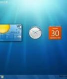

![Phần mềm ARC GIS: [Thêm từ khóa và lợi ích để tối ưu SEO]](https://cdn.tailieu.vn/images/document/thumbnail/2013/20130814/trung38dc/135x160/6611376445865.jpg)
![Gifinator: Tạo phim Stop-Motion từ thiết bị di động Android [Hướng Dẫn Chi Tiết]](https://cdn.tailieu.vn/images/document/thumbnail/2013/20130729/sunshine_10/135x160/2311375043323.jpg)
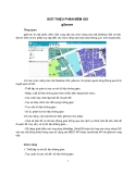


![Sổ tay Excel: Hướng dẫn sử dụng và mẹo hay [Năm hiện tại]](https://cdn.tailieu.vn/images/document/thumbnail/2026/20260520/vispacex_27/135x160/2851779253490.jpg)


%20--%3e%3cdefs%3e%3cstyle%3e%20.st0%20{%20fill:%20%23fff;%20}%20.st1%20{%20fill:%20%237800fa;%20}%20%3c/style%3e%3c/defs%3e%3cpath%20class='st1'%20d='M117.78,12.18H43.11c2.9,3.47,4.65,7.94,4.65,12.82,0,5.6-2.3,10.66-6.01,14.29h76.02l7.22-13.56-7.22-13.56Z'/%3e%3cg%3e%3cpath%20class='st0'%20d='M53.58,26.17h-.59v-1.46h.59v-4.96h2.83c1.78,0,2.67.94,2.67,2.82v5.76c0,1.87-.89,2.81-2.67,2.81h-2.83v-4.96ZM55.36,21.37v3.34h1.1v1.46h-1.1v3.34h1.01c.61,0,.91-.37.91-1.1v-5.93c0-.74-.3-1.1-.91-1.1h-1.01Z'/%3e%3cpath%20class='st0'%20d='M65.99,31.14h-1.8l-.31-2.07h-2.19l-.31,2.07h-1.64l1.82-11.39h2.62l1.82,11.39ZM65.28,18.04c-.25.46-.51.77-.75.94-.21.15-.47.22-.79.22-.26,0-.57-.07-.92-.22l-.38-.15c-.14-.05-.26-.07-.37-.07-.3,0-.53.18-.71.54l-.91-.68c.25-.46.51-.77.75-.94.21-.14.48-.21.79-.21.26,0,.57.07.92.21l.38.15c.14.05.26.07.37.07.3,0,.53-.18.71-.54l.91.68ZM61.91,27.52h1.73l-.87-5.76-.87,5.76Z'/%3e%3cpath%20class='st0'%20d='M74.53,26.89v1.52c0,1.91-.89,2.86-2.67,2.86s-2.67-.95-2.67-2.86v-5.93c0-1.91.89-2.86,2.67-2.86s2.67.95,2.67,2.86v1.11h-1.69v-1.22c0-.75-.31-1.12-.93-1.12s-.93.37-.93,1.12v6.15c0,.74.31,1.11.93,1.11s.93-.37.93-1.11v-1.63h1.69Z'/%3e%3cpath%20class='st0'%20d='M81.4,31.14h-1.8l-.31-2.07h-2.19l-.31,2.07h-1.64l1.82-11.39h2.62l1.82,11.39ZM75.9,19.2l1.52-1.91h1.71l1.51,1.91h-1.61l-.76-.95-.75.95h-1.61ZM77.32,27.52h1.73l-.87-5.76-.87,5.76ZM83.1,15.99l-1.76,1.91h-1.26l1.17-1.91h1.86Z'/%3e%3cpath%20class='st0'%20d='M84.86,19.75c1.78,0,2.67.94,2.67,2.82v1.48c0,1.87-.89,2.81-2.67,2.81h-.85v4.28h-1.79v-11.39h2.64ZM84.01,21.37v3.86h.85c.58,0,.87-.36.87-1.08v-1.71c0-.71-.29-1.07-.87-1.07h-.85Z'/%3e%3cpath%20class='st0'%20d='M93.51,19.75c1.78,0,2.67.94,2.67,2.82v1.48c0,1.87-.89,2.81-2.67,2.81h-.85v4.28h-1.79v-11.39h2.64ZM92.66,21.37v3.86h.85c.58,0,.87-.36.87-1.08v-1.71c0-.71-.29-1.07-.87-1.07h-.85Z'/%3e%3cpath%20class='st0'%20d='M98.8,31.14h-1.79v-11.39h1.79v4.88h2.03v-4.88h1.83v11.39h-1.83v-4.88h-2.03v4.88Z'/%3e%3cpath%20class='st0'%20d='M105.36,24.55h2.46v1.62h-2.46v3.34h3.09v1.63h-4.88v-11.39h4.88v1.63h-3.09v3.18ZM108.17,17.29l-1.76,1.91h-1.26l1.17-1.91h1.86Z'/%3e%3cpath%20class='st0'%20d='M112.2,19.75c1.78,0,2.67.94,2.67,2.82v1.48c0,1.87-.89,2.81-2.67,2.81h-.85v4.28h-1.79v-11.39h2.64ZM111.35,21.37v3.86h.85c.58,0,.87-.36.87-1.08v-1.71c0-.71-.29-1.07-.87-1.07h-.85Z'/%3e%3c/g%3e%3ccircle%20class='st1'%20cx='25'%20cy='25'%20r='20'/%3e%3cpath%20class='st0'%20d='M32.78,19.27c2.92,0,4.43,2.55,5.28,5.33l.71,2.17c.14.38-.33.75-.71.75h-5.61c.19-.33.24-.71.09-1.08l-.75-2.45c-.43-1.32-.99-2.64-1.79-3.77.75-.57,1.65-.94,2.78-.94h0ZM25,18.38c3.25,0,4.9,2.78,5.89,5.89l.76,2.45c.14.42-.33.8-.8.8h-11.69c-.42,0-.94-.38-.8-.8l.75-2.45c.99-3.11,2.64-5.89,5.89-5.89h0ZM25,11.35c1.74,0,3.11,1.37,3.11,3.11s-1.37,3.11-3.11,3.11-3.11-1.41-3.11-3.11,1.41-3.11,3.11-3.11h0ZM17.27,19.27c1.08,0,1.98.38,2.73.94-.8,1.13-1.37,2.45-1.74,3.77l-.8,2.45c-.14.38-.05.75.09,1.08h-5.56c-.42,0-.9-.38-.75-.75l.71-2.17c.9-2.78,2.41-5.33,5.33-5.33h0ZM17.27,12.91c1.51,0,2.78,1.27,2.78,2.83s-1.27,2.83-2.78,2.83-2.83-1.27-2.83-2.83,1.27-2.83,2.83-2.83h0ZM32.78,12.91c1.56,0,2.78,1.27,2.78,2.83s-1.23,2.83-2.78,2.83-2.83-1.27-2.83-2.83,1.27-2.83,2.83-2.83h0ZM27.07,28.56v.09c0,.57-.24,1.08-.61,1.46h0v.05c-.38.33-.9.57-1.46.57s-1.08-.24-1.46-.61h0c-.38-.38-.61-.9-.61-1.46v-.09h1.41v.09c0,.19.05.38.19.47v.05c.09.09.28.19.47.19s.38-.09.47-.19v-.05c.14-.09.24-.28.24-.47t-.05-.09h1.41ZM30.99,28.56v.09c0,1.65-.66,3.16-1.74,4.24-1.08,1.08-2.59,1.79-4.24,1.79s-3.16-.71-4.24-1.79l-.05-.05c-1.04-1.08-1.7-2.55-1.7-4.2v-.09h1.41v.09c0,1.27.47,2.4,1.27,3.25h.05c.85.85,1.98,1.37,3.25,1.37s2.4-.52,3.25-1.37c.85-.8,1.37-1.98,1.37-3.25v-.09h1.37ZM34.99,28.56v.09c0,2.78-1.13,5.28-2.92,7.07-1.79,1.79-4.29,2.92-7.07,2.92s-5.23-1.13-7.07-2.92c-1.79-1.79-2.92-4.29-2.92-7.07v-.09h1.41v.09c0,2.4.94,4.53,2.5,6.08,1.56,1.56,3.72,2.5,6.08,2.5s4.52-.94,6.08-2.5c1.56-1.56,2.5-3.68,2.5-6.08v-.09h1.41Z'/%3e%3c/svg%3e)