EURASIP Journal on Applied Signal Processing 2005:4, 471–481 c(cid:1) 2005 Hindawi Publishing Corporation
Data-Model Relationship in Text-Independent Speaker Recognition
John S. D. Mason School of Engineering, University of Wales Swansea, Swansea SA2 8 PP, UK Email: j.s.d.mason@swansea.ac.uk
Nicholas W. D. Evans School of Engineering, University of Wales Swansea, Swansea SA2 8PP, UK Email: n.w.d.evans@swansea.ac.uk
Robert Stapert Aculab, Milton Keynes MK1 1PT, UK Email: robert.stapert@aculab.com
Roland Auckenthaler School of Engineering, University of Wales Swansea, Swansea SA2 8PP, UK Email: roland@speaker-verification.com
Received 12 December 2002; Revised 23 September 2004; Recommended for Publication by Kenneth Lam
Text-independent speaker recognition systems such as those based on Gaussian mixture models (GMMs) do not include time sequence information (TSI) within the model itself. The level of importance of TSI in speaker recognition is an interesting ques- tion and one addressed in this paper. Recent works has shown that the utilisation of higher-level information such as idiolect, pronunciation, and prosodics can be useful in reducing speaker recognition error rates. In accordance with these developments, the aim of this paper is to show that as more data becomes available, the basic GMM can be enhanced by utilising TSI, even in a text-independent mode. This paper presents experimental work incorporating TSI into the conventional GMM. The resulting system, known as the segmental mixture model (SMM), embeds dynamic time warping (DTW) into a GMM framework. Results are presented on the 2000-speaker SpeechDat Welsh database which show improved speaker recognition performance with the SMM.
Keywords and phrases: speaker recognition, segmental mixture modelling.
1.
INTRODUCTION
state-of-the-art
text-independent
and speaker recognition. The instantaneous form is typically derived from a frame of speech spanning 20–30 milliseconds and is given the term atomic here to reflect the shortest prac- tical time interval over which meaningful features can be extracted. The transition features are derived from a short sequence of instantaneous features. This idea was first pro- posed by Furui in 1981 [2] using regression analysis.
The level of importance of TSI in speaker recognition is in itself an interesting question and one addressed in this paper. The focus here is on text-independent speaker recog- nition systems, defined as those that place no constraints on the contents of the spoken test utterance. TSI is the bastion of the complementary task of speech recognition, since the tem- poral sequence itself conveys the text of the spoken utterance. It is well known that as the amount of data increases, more complex models can be trained, potentially leading
speaker Most current recognition systems are based on the Gaussian mixture model (GMM), introduced by Reynolds [1] in 1992. The GMM can be viewed as a single state hidden Markov model (HMM); thus with only a single state there can be no inter- state transitions and there can be no time sequence infor- mation (TSI) within the model. TSI in this context is de- fined as information derived from the make-up of atomic speech units along the time course. Transition features, pop- ular in both speech and speaker recognition, provide an ex- ample of TSI since they measure the rate of change of the instantaneous features. The basic atomic units and these derivatives are invariably in the form of cepstra and delta cepstra, respectively, and are very widely used in both speech
472
EURASIP Journal on Applied Signal Processing
Available data
Life-time
Hours
Multisession
Session
to better recognition performance. It is interesting to note that today’s state-of-the-art speech recognition systems are trained on more speech than a human is likely to hear in a lifetime [3]. Clearly obtaining such volumes of speaker spe- cific data is impossible and hence in the task considered here, namely text-independent speaker recognition, it is argued that the model structure should reflect the amount of data available in a given situation.
Sentence Word
Atomic n-gram Classification unit
SMM
The fact that GMMs rather than HMMs underpin the state-of-the-art speaker recognition systems might be inter- preted to mean that there are negligible benefits in using TSI in this form of speaker recognition. The use of models that possess temporal properties such as HMMs has shown negligible advantages over the GMM. Supporting this view, Tishby [4], for example, reports that the Markovian transi- tion probabilities from an HMM lend negligible improve- ments to text-independent speaker recognition.
GMM HMM
Figure 1: Hypothesised recognition accuracy. As the amount of data increases, the utilisation of longer speech units becomes viable.
levels of information over longer time units. As the amount of data increases, there is an initial rapid improvement ob- tained at the atomic level of classification unit. Only when greater amounts of data are available is it likely that higher level units (extracted over longer time intervals) will con- tribute to recognition performance. At this stage the atomic- level classification can be enhanced with different structures and with higher-level information. In this paper the focus is on the region just beyond the atomic level within the shaded area in Figure 1. The aim is to show that as more training data becomes available the standard GMM is ca- pable of being enhanced and accuracy improved by utilis- ing TSI.
However, the recent works of Doddington [5] and the SuperSID workshop [6] illustrate the potential benefits of higher-level information in speaker recognition, where higher level comprises idiolect, pronunciation, and prosod- ics. Such concepts involve TSI and speech units well above the atomic level, even though the foundations might well re- main the atomic units. It is interesting to observe that in the transition from one form of information to the other, two observations are apparent, one relating to the type of infor- mation and the other relating to time; there is a clear move from formative measures close to the signal toward cognitive units such as words and phrases; in terms of time, the classi- fication units move from tens of milliseconds to seconds. The cognitive level is illustrated by comments such as a high pitch or stressed speech, enabling the listener to “know” some- thing about the speaker. A critical practical factor at the cog- nitive level is the need for large amounts of speaker specific training data. When these large quantities of data are avail- able, higher-level information can prove beneficial in speaker recognition [5, 6, 7, 8].
Of course, in practice, recognition performance is inher- ently linked to both the training and testing durations. In this paper the major theme is the model itself, its complexity and its training requirements, particularly in the context of TSI. In most applications, the training data is captured over mul- tiple sessions and is much longer than the test data. While the absolute performance of the system is a function of both testing and training data, the main theme here is the model and its training.
It is therefore likely that other forms of TSI, compris- ing short sequences of atomic units, could also prove to be beneficial in speaker recognition. These might well call for intermediate quantities of speaker specific data. So a key point here, and one addressed in this paper, is the quan- tity of data required to train the recogniser. This is likely to influence the choice of speech unit (feature) utilised in the classification. In the minimal case the atomic units are pre- dicted to perform best and when more data becomes avail- able then longer units become viable. Ultimately, systems can harness higher-level information. The dependency of higher- level systems on large amounts of training data is well il- lustrated by considering idiolectic word-level measures. In order to obtain statistics on word usage for a given speaker then relatively long and, in practise, multiple recordings are necessary, much more than has been considered historically in speaker recognition research.
The remainder of this paper is organised as follows. Section 2 discusses the data-model relationship in a purely hypothetical context. In Section 3 the approach with which TSI is harnessed is introduced. This takes the form of short segments embedded in a standard GMM configura- tion and is termed the segmental mixture model (SMM). The hypothesis put forward in Section 2 is then tested ex- perimentally on the 2000-speaker SpeechDat Welsh database [9]. Results are presented in Section 4; these compare the standard GMM to the proposed SMM in a text-independent speaker recognition context. Conclusions are presented in Section 5.
The general idea is presented in Figure 1 in which curves trace a path of hypothesised accuracy for different quan- tities of training data against different classification units, where the different classification units represent increasing
Data-Model Relationship in Speaker Recognition
473
2. DATA-MODEL RELATIONSHIP
The amount and quality of both test and training data are known to be influential factors in speaker recognition per- formance and these factors are application dependent. In the case of telephony applications, for example, the quality of data might be relatively low due to background noise and possible transmission degradations; but this can be offset by the potential for large quantities of data [10]. Thus at one end of the scale there might be just a few short utterances while at the other end of the scale there is the situation where very large quantities of data are available, both for testing and training. Radio and television broadcasting are situations where good quality and quantity of speaker specific data can be available. It would be possible to collect large quantities of data from well-known broadcasters or entertainers, build models from this data, and use these to search archives for instances of these people [11]. A recent paper by Dodding- ton [5] addresses this latter scenario of large amounts of data, and shows that word frequencies are potentially useful in dis- criminating people. This idiolectic-based approach presents an interesting contrast to the conventional spectral-based ap- proaches which have dominated the field until recently.
tens of milliseconds and a step, albeit a small one, toward the much higher level of n-grams for which the speech is likely to span much longer time intervals, in the order of seconds. As mentioned above, systems operating on longer time units tend to demand increasing amounts of data, particu- larly training data. The complexity of such models and their performance as a function of training data is now consid- ered. Figure 2 depicts the hypothetical performance of three speaker recognition systems which differ only in the quantity of data that is used for model training. Figure 2a corresponds to the least amount of data, Figure 2c the most. The plots are of recognition error rates (vertical axis) versus model size (horizontal axis). Each figure illustrates three different pro- files corresponding to different model complexities or clas- sification units and shows the effect of increasing the model size on the recognition error. In all cases the simplest model, labelled A + 0, utilises simple atomic classification units; in the context of a GMM this would be the number of com- ponents in the mixture. The other two profiles, labelled A + 1 and A + 2, illustrate the variation in speaker recognition performance as classification units utilise increasing levels of TSI, that is, implicitly over longer time intervals. Whilst the amount of data corresponding to configurations between fig- ures changes, within each figure the amount of data used for training in the different configurations is constant. The three hypothesised experiments are now discussed in turn.
As mentioned above, the GMM approach [1] can be thought of as operating on atomic levels in speech space, with potentially many thousands of components in the model. However, a speaker will display a degree of text dependency and, as a consequence, recognition systems could incorpo- rate a corresponding degree of text dependence. This raises the very interesting question of how best to harness this information. This paper is concerned with the approaches taken to speaker recognition as the amount of speech data changes. In other words, how might the optimal models change as more data becomes available?
Minimum data Figure 2a, is for a relatively small amount of training data, for example, a few seconds or a single utterance. For the least complex model, A + 0, recognition error (vertical axis) falls steadily as the model size increases and for all model sizes there is sufficient data to accurately train each model. The A + 1 profile is for a slightly more complex model, captur- ing a minimal level of TSI; again the recognition error falls steadily for the smaller model sizes. However, since the model is now moderately more complex, the same amount of train- ing data is insufficient to accurately train models of relatively larger size and thus recognition error begins to increase. The most complex model (A + 2) which captures TSI over and above that in the A + 1 profile, also falls for smaller model sizes but curves upward sooner than the A + 1 profile.
Returning to Figure 1, the profiles represent hypothesised accuracy of speaker recognition systems. For a given amount of data, illustrated on the vertical axis, contributions become feasible from different classification units, indicated on the horizontal axis. Assuming that the data available is limited to just a few short utterances, and assuming a text-independent mode, then the classification unit is likely to be on the far left of the horizontal axis, in the form of the atomic speech units. The classifier is likely to be a standard GMM or equiv- alent working directly on the atomic units of speech. Given several minutes of speech data, it might then be possible to make use of the dynamics of the speech feature sequence. This hypothesis is supported by the widespread use of transi- tional features in the classification process [2]. Transitional features capture information from the time sequence and therefore are a form of TSI. First-order derivatives are gener- ally used and give good discrimination when sufficient data is available. This might be thought of as a first small step in the use of TSI.
Immediately to the right of the GMM on the horizontal axis is the SMM [12, 13]. Here the aim is to capture TSI over and above that in the transitional speech features and to do so in the model rather than in the features. The SMM is a step away from the so-called atomic level of vectors spanning
Medium data Figure 2b shows a similar scenario to Figure 2a except that more data is now available, perhaps a few minutes or a few sentences, for example. Once again, for the least complex model, A + 0, recognition error falls steadily as the model size increases, there again being sufficient data to accurately train the model. This time, however, the profile correspond- ing to the model of medium complexity, A + 1, falls steadily and gives reduced recognition error for all model sizes con- sidered. There is now more data available, thus allowing for accurate training of slightly more complex and larger mod- els. However, for larger model sizes there is still insufficient data to accurately train the most complex model, A + 2, the profile for which again begins to curve upward for larger
474
EURASIP Journal on Applied Signal Processing
A+0 A+1 A+2
the profiles do not intersect each other. The most complex model, A + 2, consistently has the lowest error rates and the least complex, A + 0, the greatest error rates. In this case the amount of training data is large, sufficient to utilise the com- plexity of the most complex model which thus gives the best performance.
r o r r e n o i t i n g o c e R
Increasing model size
(a)
r o r r e n o i t i n g o c e R
A+0 A+1 A+2
The three figures serve to illustrate that increasing the amount of training data will not only allow larger models for fixed complexity, but also more complex ones, the poten- tial benefit of which is seen in the error rates. Note however, that in the limits of large model size and large quantities of data then ultimately the profiles must intersect, or at least converge. In the limits the optimum classifier is the nearest neighbour [14] and thus the least complex arrangement is the best when the training data tends to infinity. The hypo- thetical theme presented here is examined experimentally be- low, where the classifying unit for which the similarity score is derived is expanded from a single atomic unit in the stan- dard GMM (i.e., A + 0 in the presented hypothesis) to a short sequence of units in the SMM (i.e., A + 1 in the presented hy- pothesis).
Increasing model size
(b)
3. HARNESSING TSI
r o r r e n o i t i n g o c e R
A+0 A+1 A+2
Increasing model size
TSI is present in the temporal order of the atomic units of speech features and it is known that this information can be usefully harnessed for speaker recognition. One form of TSI is obviously present in the dynamic features that are em- ployed in almost every state-of-the-art speaker recognition system. The aim here is to capture TSI beyond that inherently present in the dynamic features. The TSI suggested here is of a different nature to dynamic features in that it is embedded in the model itself.
(c)
Figure 2: Hypothetical performance of speaker recognition utilis- ing different quantities of speaker specific data: (a) minimum data, for example, a few seconds, (b) medium data, for example, a few minutes, and (c) maximum data, for example, hours to lifetime. For each different quantity of data, three different profiles are illustrated corresponding to minimal complexity (A + 0), medium complexity (A + 1) which captures a minimal level of TSI and, maximum com- plexity (A + 2) which captures an increased level of TSI.
In order to demonstrate the potential of the two forms, dynamic features and the new model-based TSI, the two are used in combination. First the GMM baseline is established in a standard configuration utilising dynamic features. Then the model-based SMM is tested in otherwise identical condi- tions (i.e., including dynamic features) in order to establish the contribution from the model-based TSI. Model-based TSI here takes the form of short segments comprised of con- tiguous feature vectors. The duration of the segments within the SMM is a design parameter. It has to be long enough to exhibit some level of discrimination but short enough to accommodate the text-independent nature of the task. It must also reflect the amount of training data. Other practi- cal factors in TSI configurations include whether or not the segment lengths are fixed or variable and to what extent the scoring process is constrained to the temporal axis.
3.1.
Implementation
model sizes. This point represents the model size at which the amount of training data is no longer sufficient to reli- ably train all the components. The recognition errors of the A + 0 and A + 1 models continue to improve as they are less complex and the data is sufficient to reliably estimate the pa- rameters.
Maximum data Figure 2c is for a much larger amount of training data, per- haps a few hours or more. This time, for all model sizes con- sidered, the three profiles remain monotonic with the error rates dropping as the model sizes increase. Note, in this case
The proposed SMM is to provide detailed level compar- isons of short segments; in terms of implementation this can be achieved with a statistical model in the form of an HMM or a template matching process such as dynamic time warping (DTW). In many ways these two are equivalent in that DTW can be mapped to specific HMM configurations.
Data-Model Relationship in Speaker Recognition
475
The goal in training a GMM is to estimate a model λ with parameters that best match the distribution of the train- ing vectors, that is, to maximise the likelihood of the GMM, given the training data. For this purpose the expectation- maximisation (EM) algorithm is invariably used. The EM al- gorithm is an iterative process that takes an initial model, λ, and estimates a new one, ¯λ, such that p(X|¯λ) ≥ p(X|λ); the new model becomes the model for the next iteration and the process continues until some convergence criterion has been reached.
However, DTW has been preferred in the context of speaker recognition by [2, 15, 16, 17]. There are some factors in DTW which are not readily mapped into HMMs, one example be- ing repeated scoring of a given input vector. Such flexibility of the DTW template matching process possibly contributes to its preference in situations where detailed time alignment is of paramount interest and is the motivation for its choice here. DTW is embedded within the GMM, leading to the SMM. The training and testing procedures of the SMM re- main very similar to the GMM differing only by the DTW alignment scoring.
In practice, speaker specific GMMs are derived from a “world” model [20], also known as a universal background model [21]. The world model provides a means of normal- isation and compensates for the general lack of speaker spe- cific training data. Speaker specific models are generated by adapting the world model using the speaker specific data in the adaptation process.
3.3. The SMM
Many constraints may be given to a DTW system. These can be given in the form of directional restrictions, repetition restrictions, weighted movements, and global constraints. The constraints applied here allow for skips and repetitions and are similar to the widely adopted Itakura constraints in [18]. DTW provides for two normalisation processes, namely global for the overall length normalisation and local atomic unit alignments. Only the latter is relevant here since the seg- ments themselves are of the same length. Further discussions relating to DTW constraints and the context of the SMM can be found in [12].
3.2. The GMM
In the segmental mixture model each mixture component, λ, of the standard GMM becomes a short sequence of single components called a segment. Segments consist of a number of contiguous feature vectors, S. When S is one, then the sys- tem is the standard GMM. When S is greater than one, then the system is the SMM. For the SMM, the similarity measure is thus a modified form of the standard GMM measure in (1) leading to an equivalent pdf interpretation for the SMM out- put applying to segments rather than single vectors. The den- sity, given an input segment (cid:1)x, is the sum of M-weighted segment densities:
M(cid:8)
p((cid:1)x|λ) =
wibi((cid:1)x),
(3)
i=1
where wi is the segment weight and M is the total number of model components. A segment density bi((cid:1)x) is
(cid:9)
(cid:5) S(cid:7)
As mentioned previously, the standard GMM can be thought of as a single-state HMM. TSI is inherent in the conventional HMM structure in the form of state transitions which reflect the content of a specific utterance. However the basic GMM, as viewed in terms of a special case of the HMM, has only one state and hence possesses no TSI. One possibility for TSI in the text-independent mode would be an ergodic HMM with all states fully interconnected and then state transitions to- gether with state occupancy might well offer speaker specific TSI. Such ideas have been reported by Charlet [19], albeit in a text dependent mode. Alternatively, and as proposed here, the standard GMM can be modified so that a single state pos- sesses TSI. To see how this might be achieved, first the scoring process of the GMM is considered followed by the equivalent process for the proposed SMM.
(cid:4) (cid:4)Σi
dw
(4)
bi((cid:1)x) = ln
(cid:4) (cid:4)−1/2 exp
(cid:10)(cid:6) ,
− 1 2
s
Each GMM component consists of a mean, a covariance matrix, and a weight. The probability density function (pdf) of component i given the input vector (cid:1)x is given by
(cid:11)S
(cid:5)
(cid:6) (cid:2)
(cid:3)
(cid:2) (cid:1) (cid:1)x
=
(cid:2)(cid:1)Σ−1
bi
(cid:1) (cid:1)x − (cid:1)µi
(cid:1) (cid:1)x − (cid:1)µi
i
, (1)
(cid:4) exp (cid:4)
− 1 2
(cid:4) (cid:4)Σi
1 (2π)D
(cid:1)(cid:1)
(cid:2)(cid:2)
where dw is the DTW warp difference between an input seg- s |Σi|−1/2 is the prod- ment (cid:1)x and a model segment, and uct of the diagonal covariance matrices taken along the DTW warp path. S is the size of the segment measured in vectors. The DTW warp difference is given by (cid:1) (cid:2)(cid:1)Σ−1 (cid:1)xs − (cid:1)µis
(cid:1)xs − (cid:1)µis
i
dw = W S s
(5)
,
where Σi is the covariance matrix, (cid:1)µi is the mean vector, and D is the dimension of the vector.
In a simplified form, popular in practical speaker recog- nition, each component consists of a mean vector, a weight, and the diagonal of the covariance matrix on the assumption of statistical independence for the mixture components. The pdf of the input speech X given the model λ is given by
T(cid:7)
where W is the normalising term along the warp path of (cid:1)x and (cid:1)µis. The DTW process time aligns the test segments against each of the M model components. Thus for every test segment, the optimal score against each of the M model components is derived and these scores are weighted and summed as indicated in (3).
p
p(X|λ) =
(cid:2) (cid:1) (cid:1)xt|λ ,
(2)
t=1
The above serves to show how the DTW technique is em- bedded into GMM to give the new SMM and in so doing introduces TSI to the popular speaker recognition method.
where T is the total number of input vectors, (cid:1)xt.
476
EURASIP Journal on Applied Signal Processing
50 40 30
)
%
(
20
10
y t i l i b a b o r p s s i
5
M
2
0.5
0.1
The overall processes of testing and training are identical for the GMM and the SMM other than in the details of the scor- ing as indicated in (1) and (2) for the GMM and (3), (4), and (5) for the SMM. In summary the similarity measure applies to segments of vectors in the SMM rather than to single vec- tors in the GMM. The potential benefit lies in the granularity of time warping and pattern matching with short segments. The SMM can be viewed as an inverted HMM, where the overarching state transitions are moved to the heart of the similarity measure. In the implementation reported here, however, time alignment is achieved via DTW. Another valid approach would be to align the segments using HMM-style state transitions. In this case a given test segment would be scored against each of the M HMM-style submodels. Such an arrangement is a viable alternative. However, the DTW implementation is adopted here for reasons given above.
0.1 0.5 2 5 10 20 30 40 50 False alarms probability (%)
4. EXPERIMENTAL WORK
3 s 10 s 30 s
Figure 3: Detection error tradeoff (DET) profiles for a standard GMM speaker verification system with 256 components, trained on approximately 3, 10, and 30 seconds of speaker specific train- ing data. In all cases, the test is a single-digit utterance. The profiles illustrate a decreasing EER as more speaker specific training data become available.
This section presents experimental work to assess the theme under investigation in this paper, namely the benefits of TSI in speaker recognition and the training data-model relation- ship. The first set of experimental results aim to compare the performance of the standard GMM and the proposed SMM with differing amounts of training data. The second set of experiments considers SMM performance for different seg- ment and model sizes where the aim is to investigate the hy- pothesis presented in Section 2.
All experiments use data from a 2000-speaker database recorded over the public-switched telephone network [9]. Speech data from 1000 of the 2000 speakers are used to cre- ate a world model1 and the other 1000 speakers are used for speaker model training and testing. A total of about 8 hours of data is used to train a world model. Each speaker model is trained using phonetically rich sentences and experiments are conducted with approximately 3 seconds, 10 seconds, and 30 seconds of data per speaker. Testing is text-independent using one-digit utterance per speaker per test giving 1000 tests in total. Throughout, the features are standard MFCC- 14 instantaneous together with their dynamic counterparts giving a 28th-order feature.
4.1. GMM versus SMM
of false alarms the SMM is marginally better for all three lev- els of training, while the reverse is true at the low end of this scale where the GMM is better than the SMM especially for the shorter training sets. For example, with 3-second train- ing, at the extreme of 50% miss probability the false alarm rate is 0.5% and 1.5% for the GMM and SMM, respectively. The central region of the profiles, where the miss prob- ability matches the false alarm probability, leads to an often quoted measure of performance, namely the equal error rate (EER). From Figure 4 the SMM is seen to have an EER a lit- tle below 5% while for the GMM it is marginally above 5% (Figure 3). These values, along with the other EER values, are shown in Figure 5. The EER for the GMM (solid profile) and 3-segment SMM (dashed profile) are shown against the three levels of training. The two profiles illustrate that with a mini- mal level of training data (3 seconds) the GMM outperforms the SMM, whereas for greater amounts of training data (10 and 30 seconds) the SMM is better.
4.2. Data-model relationship
Figure 3 shows the baseline GMM verification results. The detection error tradeoff (DET) profile depicts the miss prob- ability against the false alarm probability and, as might be predicted, error rates reduce with increasing training data. The profiles shown are for 3 seconds, 10 seconds, and 30 sec- onds of speaker specific training data; in all cases the models have 256 components. Figure 4 shows directly equivalent re- sults for a 3-segment SMM. It is noticed that at the high end
1Similar experiments are reported in [13] in which slightly better results are presented. It was subsequently discovered that in [13], the same 1000 speakers were used in both testing and training. Here, the world model is generated from a different 1000 speakers resulting in slightly inferior recog- nition scores.
From the experimental evidence presented thus far, it is evi- dent that the SMM can outperform the standard GMM given sufficient speaker specific training data. The emphasis now moves to further assessing the performance of the SMM in terms of available data, the number of components in the model, and the sequence lengths in the SMM scoring process, that is, the segment size. It should be noted that the defini- tion of a component in the cases of the GMM and the SMM are different. In the case of the GMM, it is the conventional
Data-Model Relationship in Speaker Recognition
477
)
%
(
)
%
(
e t a r
r o r r e
l a u q E
y t i l i b a b o r p s s i
M
50 12 40 11 30 10 9 20 8 10 7 6 5 5 2 4 3 3 10 30 0.5 Training data (s)
0.1 GMM SMM 0.1 0.5 2 5 10 20 30 40 50 False alarms probability (%)
3 s 10 s 30 s
Figure 5: Speaker verification EERs (%) for the GMM (solid pro- file) and SMM (dashed profile) of Figures 3 and 4 against an amount of speaker training data in seconds. The profiles illustrate that the GMM outperforms the SMM given a small amount of speaker spe- cific training data. Given sufficient data, though, the SMM outper- forms the GMM.
Figure 4: DET profiles for a 3-segment SMM. Again the profiles illustrate a decreasing EER as more speaker specific training data become available.
components and a segment size of 3 (S3). The lowest EER is now 6.1% compared with 8.8% for 3 seconds of training data. It is now possible to reliably train slightly more com- plex models (more TSI) with more components.
Gaussian component whereas in the case of the SMM a com- ponent is not a Gaussian distribution but is comprised of a segment having more than one mean, a pooled variance, and a single weight. Nonetheless, the term model size refers to the number of components.
Experimental results are presented in Figures 6, 7, 8, and 9 which show EER profiles against model size (a) and against segment size (b) for each of four training conditions. Again lengths of 3, 10, and 30 seconds of phonetically rich sentences are used. In addition, to utilise the database to the full, the 30-second case is extended by digit string utterances giving a total of approximately 40 seconds per speaker.
Moving to Figure 8, where there is now 30 seconds of training data, again the EER drops to a minimum of 4.3% for S3 and model size 256. S3 now has the lowest profile for model sizes 64 and beyond. From Figure 8b it is clear that all model sizes beyond 32 show benefits of the SMM over the standard GMM with S3 being the best. Again, more data means more complex, larger models give better performance. Finally, Figure 9 shows equivalent profiles for 40 seconds of speaker specific training data. Again, all but the smallest models benefit from the SMM structure. The lowest point on the profiles now corresponds to S5 and a model size of 512 with an EER of 3.5%. The trend implies that as more speaker specific data becomes available, the merits of the SMM in- crease as predicted by our earlier hypothesis. From (a) the S3 and S5 SMMs outperform the standard GMM (S1) for all model sizes greater than 32 components.
In terms of the data-model relationship it is noticed that, for 3 seconds of training data (Figure 6), the optimum model size is 64 with a distinct trough for a segment size of 3. As more data becomes available the troughs broaden and the benefits of the SMM become more apparent. This trend is evident for all three segment sizes.
Figure 6 illustrates verification performance with a min- imal amount of speaker specific data (3 seconds). Figure 6a shows that segments of 1 and 3 give very similar scores for model sizes of 64 and 128, with the profile for S3 being marginally below that for S1 for these two cases. Further- more, the model size of 64 gives a minimum for each of the three segment sizes. Figure 6b gives an alternative view with the EER plotted against segment size showing more clearly any performance improvements as the segment size increases. In this case, with just 3 seconds of training data, only for model sizes of 64 and 128 is there any merit of the SMM over the GMM (S1 corresponds to a segment size of 1, i.e., the standard GMM; S3 and S5 indicate segment sizes of 3 and 5, resp.). There is thus insufficient data to reliably train models with greater than 64 components or more complex models (i.e., that capture more TSI) than the standard GMM. Verification performance with 10 seconds of speaker spe- cific training data is illustrated in Figure 7. The fall in EER is immediately apparent. Figure 7a shows that the best per- formance is obtained with models of between 64 and 256
The SMM profiles are steeper in all cases for the smallest and largest model sizes. Clearly this sensitivity to model size is a disadvantage in practice. However, for relatively larger amounts of training data over a few minutes or more, the trend of the curves suggest that the SMM would be superior over a reasonable model size range (model sizes over 32).
478
EURASIP Journal on Applied Signal Processing
)
)
%
%
(
(
e t a r
e t a r
r o r r e
r o r r e
l a u q E
l a u q E
12 12 11 11 10 10 9 9 8 8 7 7 6 6 5 5 4 4 3 3 8 16 32 64 128 256 512 1024 S1 S3 S5 Model size Segment size
Set, S1 Set, S3 Set, S5 Model size, 8 Model size, 16 Model size, 32 Model size, 64 Model size, 128 Model size, 256 Model size, 512 Model size, 1024
(a) (b)
Figure 6: Speaker verification EER with 3 seconds of speaker specific training data. (a) EER against model size. The three profiles correspond to the SMM with 1, 3, and 5 segments. (b) EER against segment size. The eight profiles then correspond to different model sizes. With 3 seconds of training data, the S1 profile gives the best or as good performance as S3 and S5. The optimum model size is 64 components which corresponds to an EER of 8.8%.
)
)
%
%
(
(
e t a r
e t a r
r o r r e
r o r r e
l a u q E
l a u q E
12 12 11 11 10 10 9 9 8 8 7 7 6 6 5 5 4 4 3 3 8 16 32 64 128 256 512 1024 S1 S3 S5 Model size Segment size
Set, S1 Set, S3 Set, S5 Model size, 8 Model size, 16 Model size, 32 Model size, 64 Model size, 128 Model size, 256 Model size, 512 Model size, 1024
(a) (b)
Figure 7: Speaker verification EER with 10 seconds of speaker specific training data. The extra data is now sufficient to train a slightly more complex model, S3, which gives the best performance for models with 64 to 256 components corresponding to an EER of 6.1%.
5. CONCLUSIONS
Perhaps the surprising characteristics of the SMM perfor- mance is at the low model sizes where the accuracy is worse than that for the standard GMM in cases below 32 compo- nents. This conflicts with our earlier hypothesis depicted in Figure 1 and is not easily explained. Of course at the higher level of information where n-grams and word frequencies are used, the model size must be sufficient to represent the per- sons under test. So in this case, very small model sizes would not work.
Over the last decade, the GMM has become established as the standard classifier for text-independent speaker recog- nition. It operates on atomic levels of speech and can be effective with very small amounts of speaker specific train- ing data. It is clear from recent developments that when very large amounts of this data are available, higher-level information, utilising speech units well above the atomic
Data-Model Relationship in Speaker Recognition
479
)
)
%
%
(
(
e t a r
e t a r
r o r r e
r o r r e
l a u q E
l a u q E
12 12 11 11 10 10 9 9 8 8 7 7 6 6 5 5 4 4 3 3 8 16 32 64 128 256 512 1024 S1 S5 S3 Model size Segment size
Set, S1 Set, S3 Set, S5 Model size, 8 Model size, 16 Model size, 32 Model size, 64 Model size, 128 Model size, 256 Model size, 512 Model size, 1024
(a) (b)
Figure 8: Speaker verification EER with 30 seconds of speaker specific training data. Even with 30 seconds of data, the S3 SMM still gives the best performance, but the amount of data is now sufficient to train a model with 256 components which gives a reduced EER of 4.4%.
)
)
%
%
(
(
e t a r
e t a r
r o r r e
r o r r e
l a u q E
l a u q E
12 12 11 11 10 10 9 9 8 8 7 7 6 6 5 5 4 4 3 3 8 16 32 64 128 256 512 1024 S1 S3 S5 Model size Segment size
Set, S1 Set, S3 Set, S5 Model size, 8 Model size, 16 Model size, 32 Model size, 64 Model size, 128 Model size, 256 Model size, 512 Model size, 1024
(a) (b)