EURASIP Journal on Applied Signal Processing 2005:7, 1071–1081 c(cid:1) 2005 Hindawi Publishing Corporation
Perception SoC Based on an Ultrasonic Array of Sensors: Efficient DSP Core Implementation and Subsequent Experimental Results
A. Kassem PolySTIM Neurotechnology Laboratory, Department of Electrical Engineering, ´Ecole Polytechnique de Montr´eal, Case Postale 6079, Succursale Centre-ville, Montr´eal, QC, Canada H3C 3A7 Email: abdallah.kassem@polymtl.ca
M. Sawan PolySTIM Neurotechnology Laboratory, Department of Electrical Engineering, ´Ecole Polytechnique de Montr´eal, Case Postale 6079, Succursale Centre-ville, Montr´eal, QC, Canada H3C 3A7 Email: mohamad.sawan@polymtl.ca
M. Boukadoum Department of Computer Sciences, Universit´e du Qu´ebec `a Montr´eal, Case Postale 8888, Succursale Centre-ville, Montr´eal, QC, Canada H3C 3P8 Email: boukadoum.mounir@uqam.ca
A. Haidar Department of Computer Engineering and Informatics, Beirut Arab University, P.O. Box 11-5020, Beirut 1107 2809, Lebanon Email: ari@bau.edu.lb
Received 10 October 2004
We are concerned with the design, implementation, and validation of a perception SoC based on an ultrasonic array of sensors. The proposed SoC is dedicated to ultrasonic echography applications. A rapid prototyping platform is used to implement and validate the new architecture of the digital signal processing (DSP) core. The proposed DSP core efficiently integrates all of the necessary ultrasonic B-mode processing modules. It includes digital beamforming, quadrature demodulation of RF signals, digital filtering, and envelope detection of the received signals. This system handles 128 scan lines and 6400 samples per scan line with a 90◦ angle of view span. The design uses a minimum size lookup memory to store the initial scan information. Rapid prototyping using an ARM/FPGA combination is used to validate the operation of the described system. This system offers significant advantages of portability and a rapid time to market.
Keywords and phrases: perception SoC, ultrasonic, focusing, beamforming, DSP, FPGA circuit techniques.
1.
INTRODUCTION
mur length of the fetus. It is also used to visualize the heart, and measure the blood flows in arteries and veins [2].
The ultrasonic diagnostic imaging systems are mostly operated in the pulse-echo mode. The transducer is used both for transmitting an ultrasonic pulse into the objects and receiving the return echoes from those objects. The pulse-echo systems can be classified as A, B, or M modes. The first display mode, called A-mode (A for amplitude), is 1D display ultrasonic imaging. It displays the amplitude according to the depth of the received echoes. The second one, B-mode (B for brightness), is 2D display ultrasonic imaging which consists of pixels. The brightness of each pixel is determined by the amplitude of the received echo.
Ultrasound imaging is an efficient, noninvasive, method for medical diagnosis. Employed ultrasound waves allow to ob- tain information about the structure and nature of tissues and organs of the body [1]. They are generated by convert- ing a radio frequency (RF) electrical signal into mechanical vibration via a piezoelectric transducer sensor. The frequen- cies of these ultrasound acoustic waves are located above the 20 kHz sensitivity limit of the human ear. Among the applica- tions of ultrasound imaging, it is extensively used in obstet- rics to estimate the size and weight of a baby by measuring the head diameter, the abdominal circumference, and the fe-
1072
EURASIP Journal on Applied Signal Processing
(cid:1)
s r o s n e s d n u o s a r t l
U
(ASIC) (FPGA) (FPGA) (ASIC) Front-end DSP Video processing LPF TGC ADC Magnitude To DBF A(t) = I 2(t) + Q2(t) display Transmitter and receiver ... ... Compression and scan converters I IQ demodulator Q LPF TGC ... TGC ADC ... ADC
Controller
Figure 1: Perception SoC of the B-mode processing of the ultrasonic imaging system.
Finally, M-mode (M for motion) is 2D display ultrasonic imaging; it displays the depth in tissue according to time of the received echoes. The amplitude of the echoes is measured at a given number, of depths.
In this paper only the B-mode is considered due to the popularity in the echography industry of the brightness of imaging display.
The latter are used to generate and detect pulsed ultrasonic echoes. The received echoes are preamplified, digitalized, and passed on to a digital signal processor (DSP) block by the re- ceiver front-end [12]. This DSP core performs beamforming, quadrature demodulation, filtering, and envelope detection of the received echoes. The scan converter resamples the am- plitude of the obtained video signal in order to convert it to pixel brightness on a rectangular display screen [14]. A con- troller synchronizes the sweeping of the image area, and the transmission, reception, digitization, and displaying of the acquired data.
B-mode processing involves signal acquisition, echo sig- nal processing, and display. In the signal acquisition stage (also called the front-end), the acoustic echoes received from the tissues are converted to electrical signals by the trans- ducer. These signals are amplified with a variable gain (TGC, time-gain-compensation) that depends on the scan depth and, then, they are digitalized by the analog-to-digital con- verter (ADC) circuit.
3. ARCHITECTURE OF THE DSP CORE
The majority of commercially available ultrasonic sys- tems occupy large spaces in clinic rooms; their power con- sumption may exceed hundreds of watts and they are mainly used near the bedsides of patients. Most units are built with discrete components mounted on several printed cir- cuit boards [3], with software drivers used to control them [4]. More recently, several research efforts are being made to minimize the size of such systems by combining multi- ple processors with dedicated components, but the dimen- sions of improved devices still miss the required hand-held format [5, 6, 7, 8, 9, 10, 11]. The current efforts are moti- vated by advances in microelectronics that make it possible to design and implement an SoC that allows to build hand- held devices. Our work dedicated to build an echography de- vice follows this approach. It aims to develop a compact DSP core as the main computing engine of an ultrasound imag- ing system and first prototype it on a programmable logic device (FPGA) subsequent to an SoC device. This miniatur- ization enables a design with low power consumption, low noise, and light weight [12].
The DSP core performs the DBF to achieve the dynamic fo- cusing and steering of the received echoes. This DSP core includes also a digital IQ demodulator to remove the high- frequency carrier and reduce noise by quadrature demodu- lation. It results in in-phase (I) and quadrature (Q) samples of a complex signal I(t) + jQ(t). After lowpass filtering, the envelope (magnitude) of the received echo at time t is com- puted [9]:
(cid:2)
I 2(t) + Q2(t).
(1)
A(t) =
In this paper, we describe in Section 2 the general de- scription of the ultrasonic perception SoC. The DSP core architectural features, and its various stages, sensing front- end and its digital beamforming (DBF) module, quadrature demodulation, LPF, and envelope detection are subjects of Section 3. Section 4 contains the implementation process of the DSP core in an FPGA and its experimental results. Finally, conclusion is given in Section 5.
2. GENERAL DESCRIPTION OF THE ULTRASONIC PERCEPTION
Perception SoC can integrate functionally different compu- tational elements traditionally built around several mixed- signal ASICs and FPGAs [13]. Figure 1 shows the ultra- sonic perception SoC of the B-mode processing of the imag- ing system. The emitter generates high-voltage pulses to excite a transducer that is composed of multielement sensors.
Usually, the obtained signal has a large dynamic range, 70 dB or higher, while a typical display monitor has a dynamic range of only 35–40 dB, compatible with human vision. As a result, the dynamic range of the received echoes may be compressed before feeding them to the scan conversion stage. The required compression can be achieved by implement- ing a logarithm function [11]. Finally, the compressed signal is scan-converted from beam-space to a standard Cartesian grid [5, 15, 16] and stored in a 2D image memory, which serves for display. The controller is also responsible for in- teracting with the user, so that operating parameters such as imaging depth, gain, mode, and thresholds may be set in real- time according to the operator’s desires.
Perception SoC Based on an Ultrasonic Array of Sensors
1073
· · ·
r e d d A
Sounds Sensors Delay line dN/2 0 FP 0 Body organ d3 d2 1 d1 1 d0 2 2 f (t) 3 3 0 1 2 3 N/2 4
Pulse generator . . . N/2 4 ... N Preamp & ADC Preamp & ADC Preamp & ADC Preamp & ADC Preamp & ADC ... Preamp & ADC 2 (a)
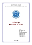
Figure 3: Simplified schematic of the pipelined digital beamform- ing.
(cid:3)
· · ·
∆N/2 ∆3 ∆2 ∆1 ∆0
3 2 1 0 N/2
The focusing process can be accomplished by using ana- log discrete components, but such an approach does not al- low to deliver the precise delays, and it generally results in a complex and bulky circuitry [18]. To improve the quality of the acquired images, analog circuit implementations as well as software calculations must be avoided. Instead, DBF tech- nique is used. Its implementation can be based on sampled- delay focusing (SDF), which consists of combining memories (FIFO) to delay and store the sampled signals, and lookup ta- bles (LUT) that contain precalculated scan lines [17, 19]. In order to improve the system design, pipelined SDF technique can be adopted to implement the variable delay without us- ing FIFO memories and with a minimum of LUTs.
3.1.1. Delay variation
(b)
Figure 2: Beamforming: (a) resulting focal point, and (b) delay generation.
Figure 3 illustrates echoes coming from a specific point (fo- cal point-FP) that are preamplified, digitized, adequately de- layed, and then added to produce a focused signal. The fo- cused signal f (t) can be expressed as [19]
N/2(cid:4)
(cid:5)
(cid:6)
3.1. Digital beamforming
Xn
t − τn
f (t) =
,
(2)
n=−N/2
where Xn is the received echo from the nth sensor element, N + 1 is the total number of sensors, and τn is the focusing and steering delay required for the nth element at depth R and is driven by
(cid:13)
(cid:11)
(cid:11)
(cid:12)
(cid:12)2
(cid:7)(cid:8) (cid:9) (cid:10)
τn =
+ 2
1 +
sin θ − 1
,
(3)
R c
nd R
nd R
where c = 1540 m/s is the average propagation speed of sound in the medium, d is the sensor spacing, and θ is the steering angle (Figure 4) [19].
For ultrasound medical imaging, ultrasonic pulses are sent into a patient’s organ and the resulting reflections (echoes) from tissues are detected by an array of sensors. One impor- tant step is the electronic dynamic focusing and steering of the echoes by means of a phased transducer array to meet the quality of the real-time processes [17]. The geometrical approach is used to realize focusing and steering by insert- ing a variable time delay after each transducer element in the array to compensate echoes for different arrival times. Using such an array of sensors transducer, the beam is fo- cused and steered by exciting each one of the array sensors at specific time. As a result, the resulting sound waves coming from all sensors arrive simultaneously at a given focal point, during the transmission. Figure 2a shows an example of this principle. During reception, a beam focusing must also be accomplished; the signals coming into the ultrasound scan- ner from the various sensors must be delayed to arrive at the same time, as shown in Figure 2b.
After exciting the sensor array, a signal is transmitted with the steering angle θ and, then, echo signals are prop- agated back from the focal point to the sensors. The distance from the focal point to the sensor located in the center of the array is R and it is different from the distance to a sensor
1074
EURASIP Journal on Applied Signal Processing
· · · Delay N/2
Delay 1 Delay 2 Focal point pointer Controller R2 Focal point Delay calculation block (DCB) LUT sin(θ) values R1
Figure 5: Proposed delay calculation architecture.
R R
−N/2 · · · −4 −3 −2 −1
θ L
0 1 2 3 4 · · · N/2
d Sensor array
maximum time to sample one scan line is tMAX(2R/c = 260 microseconds), which corresponds to 6400 samples at 50 MHz. For the whole 128 scan lines (SL), the total scan time needed is 128×260 microseconds (0.033 second), cor- responding to one frame of the scanned image. The memory required to store this image is 128×6400×8 bits/sample = 800 Kbytes.
To minimize the operations of the delay calculation, (3)
Figure 4: Dynamic focusing and steering delay.
can be modified as follows:
(cid:14)(cid:2)
(cid:15) R2 + (nd)2 + 2ndR sin θ − R
(cid:14)(cid:2)
(4)
element located at another position (R + L), where L is the propagation distance (Figure 4).
.
(cid:15) (R + nd)2 − ndR(2 − 2 sin θ) − R
τn = 1 c = 1 c
As shown in (4), the division-by-R and one multiplication operation were eliminated, thus reducing the complexity of the required hardware.
3.1.2. Pipelined sampled-delay focusing
implementation
The most important factors in implementing the pipelined SDF are the number of registers and the registers control. For each channel i of the transducer, there is a variable number of registers Regi [25]:
(cid:11)
(cid:12)
,
(5)
Regi = fs
Ln − Li c
where Ln is the maximum distance delay, n is the nth array channel and Li is the distance delay of ith channel, and fs is the sampling frequency. The maximum number of registers is determined by the sampling frequency fs and the maxi- mum distance delay of the array channel:
(cid:11)
(cid:12) .
= fs
(6)
RegMAX
Ln c
The delay information for a complete scan line can be precalculated and stored in a lookup table, using a first-in- first-out (FIFO) memory with a sampling clock generator (SCG) [19]. In a typical ultrasound image, a sector is formed of 128 beams (scan lines) and corresponds to a propagation depth of about 20 cm. The total memory requirement for such case to store the precalculated delays is about 1 Mbytes per channel (sensor), assuming that the sampling time res- olution used for focusing the phased array is 10 times if the selected transducer center frequency is 5 MHz. This would require a large memory [20, 21, 22, 23]. To resolve this prob- lem, a pipelined sampled-delay focusing architecture is used. The variable delay circuit architecture is shown in Figure 5. It includes a controller, a simplified lookup table that stores sin(θ) values, where θ is the rotation angle with values between −45◦ and 45◦, with a step of 0.7◦, the next focal point (FP) pointer calculation block and the delay cal- culation block (DCB) are activated by the controller. At the same time, the initial FP value (R) is delivered to the DCB. The delay (τn) defined in (3) is computed for the line delay of each array element and for specific angle and FP. The next FP is determined in parallel when computing τn and delivered to the DCB, and this operation is repeated M sampled times to produce a complete scan line, where M is the sampled pixel per scan line. For each angle, a scan line is formed to pro- duce a scanned image frame. To reduce the delay quantiza- tion error, and to obtain precise sampling values, fast digital circuitry is required, and the ADC must have a fast conver- sion rate. In our design, the clock frequency is 50 MHz which corresponds to 10 times if the transducer selected center fre- quency ( f0) is 5 MHz [24].
Note that the number of registers required for each channel of the transducer array varies from zero to the maximum value RegMAX. To implement such pipelined SDF, we use a counter, variable registers, and an adder, assuming that the data is coming from an array of ADCs, as shown in Figure 6. For each channel, the data acquisition is valid at the trans- ducer when the time distance 2(R + Li) is attained, where i = 0, . . . ,n, L0 = 0 is the free delay, and Li is the time dis- tance of channel i (this distance is the 2-way sound trip from the transducer to the FP). This data is controlled by a main counter and a comparator at each channel. The sequences of
As an example, assume the following conditions: array aperture (Nd) of 20 mm, scanning angle (θ) varying be- tween +45◦ and −45◦, scanning done to a depth (R) of 20 cm, and transducer center frequency ( f0) of 5 MHz. The
Perception SoC Based on an Ultrasonic Array of Sensors
1075
X 0 U
X 1 . . U . M
m u S
−
√
(cid:1)
X N/2 . U . . M
CLK Count out Counter d Sel n R 2 − 2 sin(θ) ndR CLK = fs = 50 MHz 2R R + nd nd Cmp MUX MUX Number of pipelined registers Count out ≥ 2R Reg CH (0) Reg Oper (×, +) ADC Ln c/ fs . .. M CLK Reg Count out 2(R + L1) θ CLK Cmp Count out ≥ 2(R + L1) DEMUX (R + nd)2 ndR(2 − 2 sin(θ)) CH (1) ADC Ln − L1 c/ fs Reg Reg CLK .. . θ (R + nd)2 − ndR(2 − 2 sin(θ)) Count out 2(R + Ln) CLK Cmp Count out ≥ 2(R + Ln) R + Ln = (R + nd)2 − ndR(2 − 2 sin(θ)) CH (n) ADC Ln − Ln c/ fs
Figure 7: Block diagram of the delay time distance calculation.
CLK θ
Figure 6: Block diagram of the pipelined sampled-delay.
signal, the sampling rate must be greater than twice the max- imum signal frequency, according to the Nyquist criterion. However, since the bandwidth of the envelope is less than that of the received signal, it is possible to reduce the sam- pling rate accordingly. This can be achieved by using the quadrature sampling method, which splits a band-pass sig- nal into in-phase and quadrature baseband components, and each of them is sampled separately [17]. Such bandpass sig- nal can be expressed by
(cid:16)
(cid:17)
(8)
f (t) = A(t) cos = AI (t) cos
+ AQ(t) sin
(cid:6) ,
w0t + ϕ(t) (cid:6) (cid:5) w0t
(cid:5) w0t
sampled data are inserted into the variable registers at each clock cycle. As a result of the variable registers, the echo sig- nals that were sampled at different times to compensate for different propagation path delays will be aligned at the out- put of each variable register and they will be summed to ob- tain the focused signal. For each angle, the counter and all the variable registers are reset, and the outputs of these reg- isters are selected according to the specific pipelined registers (Regi) [25]. The time distance for each channel can be com- puted by (7) adapted from (4):
where
(cid:2)
(cid:2)
Ln + R =
R2 + (nd)2 + 2ndR sin θ
A2
A(t) =
(cid:2)
(7)
Q(t), (cid:19)
=
(9)
(R + nd)2 − ndR(2 − 2 sin θ).
.
ϕ(t) = tan−1
I (t) + A2 (cid:18) AQ(t) AI (t)
In (8), ω0 and ϕ(t) are the center frequency of the trans- ducer and its phase, and AI (t) and AQ(t) are the envelopes of the in-phase and quadrature-phase components. They are obtained by mixing the bandpass beamformed signal with sine and cosine references, and subsequently are lowpass fil- tered (Figure 8). Since AI (t) and AQ(t) are baseband signals, they may be sampled at their bandwidth rate [26]. The en- velope detection is achieved by evaluating A(t) where t is re- placed by KTs, where
.
Ts ≤
(10)
1 bandwidth
For each angle, a scan line is formed to produce a scanned image frame. The distance times (Li + R) are calculated in series from L1 to Ln for each element. As an example, as- sume the same conditions as defined in the previous sec- tion with a distance spacing between channels of 0.154 mm (d = λ/2) for 129 channels (sensors) and starting scan line from 10 mm (R = a/2). The delay time distance before starting the first sample of the scan line is 2(R + Li) where L0 = 0, L1 = 131 µm, . . . , L64 = 8450 µm, and the number of pipelined registers is zero registers for channel 64, 4 regis- ters for channel 63, and the number is 274 registers for chan- nel 0 according to (5). By scheduling few operations, (7) can be realized as shown in Figure 7, which gives an optimized pipelined architecture.
3.2. Quadrature demodulation and
envelope detection
The implementation of the IQ demodulation is accom- plished by using two lookup tables for the sine and cosine, with a finite impulse response (FIR) digital lowpass filter (LPF). Finally, the Cordic method can be used to detect the envelope of the echoes [27, 28].
The received echo is envelope-detected signal after focus- ing by the DBF. To reconstruct the envelope of the received
1076
EURASIP Journal on Applied Signal Processing
I (kTs) + A2
Q(kTs)
x(n) Demodulator LPF I Magnitude (cid:2) cos(w0kTs) DBF xaN−1 xaN−2 xa1 xa0 A2 Q LPF A(kTs) = y(n) T T T sin(w0kTs) + + +
(a)
Figure 8: Quadrature sampling technique for bandpass signals.
T T
3.3. Digital filter
x(n) T T T
+ + +
Equation (11), represents the FIR filter transfer function in the time domain [29, 30]:
N −1(cid:4)
xap xa0 xa1 xap−1 y(n) + + +
y(n) =
aix(n − i − 1).
(11)
i=0
(b)
Figure 9: Realization of FIR filter: (a) simple direct structure and (b) direct structure for a linear phase filter.
In this equation, N data memories are required to hold the intermediate results and, for each output of index n, N mul- tiplications and N − 1 additions have to be performed [30]. By designing a linear phase filter, the symmetry of the coef- ficients allows to reduce by half the number of multiplica- tions. Figure 9 shows a realization of the filter and the corre- sponding structure when the number of coefficients is odd. To minimize the memory size required to implement the fil- ter, we used the minimum possible number of bits such that the characteristics of the filter are not affected for both the input data (16 bits) and/or the coefficients (12 bits).
For the needed LPF for our application that requires a sampling frequency of 50 MHz, and a cut-off frequency of 5 MHz, the transition bandwidth is 4 MHz and the stop band attenuation is greater than 35 dB. To design such a filter, Mat- lab was used to simulate the required 23rd order.
as shown in Figure 10. These data are the sampled signals from all eight channels of the ADC array, where each sample is 8 bits wide. The ARM processor writes and reads the sam- pled data via the AMBA bus at a 100 MHz clock frequency (HCLK). Because of the 50 MHz sampling period of the DSP core, each read/write cycle from the ARM processor must be divided by two to meet the DSP sampling period (50 MHz). The DSP module, programmed in the FPGA, reads the data from the AMBA bus, computes the digital beamforming, eliminates the high frequency and maintains the phase-angle by IQ demodulating and digital lowpass filtering, and finally, produces the magnitude received signal.
4.
IMPLEMENTATION OF THE DSP CORE
The DSP core requires a 50 MHz clock (CLK) that is de- rived from the main HCLK clock. HCLK is generated using one of the ICS525 programmable oscillators integrated on board of the logic module. Table 1 summarizes the DSP core parameters, and the operation of the system is as follows:
(i) the ARM processor sends data (32 bits) across the
AMBA bus at the effective rate of HCLK;
(ii) a frequency divider generates CLK from the HCLK; (iii) each 2 HCLK clock cycles, a data of 64 bits is inputted
to the DSP core module;
In order to validate the proposed architecture of the DSP core, a front-end of eight sensors was simulated and imple- mented. There were three main steps achieved: (1) Simulink model study using Matlab, (2) VHDL code generation us- ing Synospys, and (3) hardware implementation using the ARM Integrator/LM logic module rapid prototyping plat- form (ARM-RPP). The Matlab simulation was performed in a DSP core composed of 9 modules. They are the image in- put matrix, the input delay, the beamforming block, the IQ demodulation, the lowpass filter, the envelope detector, the logarithmic compressor, the decimator, and the image out- put matrix.
(iv) each 64-bit data is separated into eight 8-bit words data, which represent the output sampled data from the eight ADC channels;
(v) the data is processed at a clock rate of 50 MHz in the
DSP core module;
(vi) the ARM processor receives data from AMBA bus, and
processes it at 2 HCLK clock cycles.
A hardware reset initializes the whole system. Then, the counter addresses of the sine/cosine LUTs and all FIFO regis- ters are set to zero and R is set to its minimum value (10 mm).
The ARM-RPP platform contains an ARM7TDMI pro- cessor and a Xilinx Virtex II FPGA which provides logic and core modules. The logic module contains the FPGA, SSRAM, connectors, and several interface circuits. The core module contains an ARM processor and some configurations, and in- terface circuits. The communication between these modules is possible via a 32-bit bidirectional bus (AMBA). Due to this limitation, a modified block diagram of the ARM platform is done to produce 64-bit data as input in the DSP block,
Perception SoC Based on an Ultrasonic Array of Sensors
1077
Logic module Core module Data out
X U M E D
s u b A B M A
32 D Q Data 32 Data in/out ARM 64 32 D Q Virtex II FPGA (DSP)
D CLK = 50 MHz ¯Q Interface circuit User interface HCLK = 100 MHz
Figure 10: Block diagram of the ARM platform used for DSP core implementation.
Table 1: DSP core parameters.
Notation f0 fs fCLK θ
SL D∗∗ d R n
Parameter name Center frequency ADC sampling frequency DSP clock frequency Angle of view Number of scan lines Number of sampled data per scan line Distance between sensors Maximum distance Number of sensors
Value 5 50 50 90◦ 128 6400 0.154 200 8
Unit MHz MHz MHz Degree N/A∗ N/A∗ mm mm N/A∗
∗N/A = Not applicable. ∗∗According to this table setting.
5. SIMULATION AND EXPERIMENTAL RESULTS
the ARM-RPP platform, and after logarithmic compression using Matlab simulation. Also, this figure shows that when the number of ADC channels increases, the image resolution increases too. The number of the ADC channels used in this application is eight due to the ARM bus limitation which is 32 bits, as explained in the previous section.
Functionality of this prototype has been tested on a Xilinx FPGA, satisfying all timing constraints for the re- quired application. The timing requirements for 30 frames at 50 MHz sampling frequency is 0.5 second. Moreover, tim- ing results for FPGA implementation show that higher data rate could be operated correctly for 60 frames/s.
To test the implemented design, a phantom fetus image was generated by the Field-II ultrasound simulation software program [31, 32]. Then, the simulated image data in polar coordinates (R, θ) was inputted to the DSP core. All sam- pled data were stored in files corresponding to the data of the ADC channels, including the estimated delay of each channel at the transmission. These data were organized as one col- umn of 128×6400 values. The first 6400 values represented the first sampled scan line at −45◦, while the last 6400 val- ues represent the last sampled scan line at +45◦ for each file. The ARM processor retrieves the sampled data values from the previously created files, and sends them to the DSP core prototype via the AMBA bus. The DSP processes the sampled data and produces the magnitude values, which are saved in a new file by the ARM processor.
The DSP prototype occupies 61% (314 535 gates) of the XCV2000E FPGA, including the AMBA protocol and inter- face drivers. Table 2 summarizes the implementation results such as the needed area and the timing constraints. Finally, using this prototype, we could demonstrate that the pro- posed DSP core architecture works properly and can be ef- ficiently integrated for the purpose of building a perception SoC.
Prior to building a hardware prototype on the ARM-RPP, a Matlab model using a fetus image was implemented and simulated in order to familiarize us with the DSP core archi- tecture. The model used a depth range of 1–20 cm, and a view angle of 90◦.
6. CONCLUSION
To demonstrate the flexibility of the DSP core, the sim- ulations are done using 2, 4, and 8 ADC channels. Figure 11 illustrates the fetus images created by taking the values from the DSP prototype for 2, 4, and 8 ADC channels, built around
A perception SoC based on an array of sensors dedi- cated for ultrasound imaging system is reported. It is an
1078
EURASIP Journal on Applied Signal Processing
×103
1
2
3
4
5
6
20 40 80 100 120 60
×103
(a)
1
2
3
4
5
6
20 40 80 100 120 60
×103
(b)
1
2
3
4
5
6
60 20 40 80 100 120
(c)
Figure 11: Images produced by ARM data using (a) 2 ADC channels, (b) 4 ADC channels, and (c) 8 ADC channels.
uses an FIFO register and some LUTs to store the cosine and sine angle requirements.
implementation for an efficient DSP core. Also, subsequent experimental results are demonstrated. The DSP core is based on the digital beamforming, digital IQ demodula- tion, LPF, and envelope detection. The proposed system was implemented in a reduced complexity architecture that only
The proposed architecture reduces the complexity and the needed memory and increases the performance of the processed images by taking multirate sampling. The
Perception SoC Based on an Ultrasonic Array of Sensors
1079
Table 2: Report from implemented DSP core in the Xilinx Virtex II FPGA.
0 223
Using target part “v2000efg680-6.” Design summary: Number of errors: Number of warnings: Logic utilization:
31%
Total number of slice registers: Number used as flip flops: Number used as latches: Number of 4-input LUTs:
47%
11 936 out of 38 400 10 334 1 602 18 349 out of 38 400
Logic distribution:
Number of occupied slices: Number of slices containing only related logic: Number of slices containing unrelated logic:
14 850 out of 19 200 14 850 out of 14 850 0 out of 14 850
77% 100% 0%
∗See notes below for an explanation of the effects of unrelated logic.