Hindawi Publishing Corporation EURASIP Journal on Advances in Signal Processing Volume 2007, Article ID 13659, 8 pages doi:10.1155/2007/13659
Research Article A Hub Matrix Theory and Applications to Wireless Communications
1 Harvard School of Engineering and Applied Sciences, Harvard University, Cambridge, MA 02138, USA 2 US Air Force Research Laboratory, Rome, NY 13440, USA
H. T. Kung1 and B. W. Suter1, 2
Received 24 July 2006; Accepted 22 January 2007
Recommended by Sharon Gannot
This paper considers communications and network systems whose properties are characterized by the gaps of the leading eigen- values of AH A for a matrix A. It is shown that a sufficient and necessary condition for a large eigen-gap is that A is a “hub” matrix in the sense that it has dominant columns. Some applications of this hub theory in multiple-input and multiple-output (MIMO) wireless systems are presented.
Copyright © 2007 H. T. Kung and B. W. Suter. This is an open access article distributed under the Creative Commons Attribution License, which permits unrestricted use, distribution, and reproduction in any medium, provided the original work is properly cited.
1. INTRODUCTION theory and our mathematical results to multiple-input and multiple-output (MIMO) wireless systems.
2. HUB MATRIX THEORY
⎛
⎞
It is instructive to conduct a thought experiment on a com- putation process before we introduce our hub matrix the- ory. The process iteratively computes the values for a set of variables, which for example could be beamforming weights in a beamforming communication system. Figure 1 depicts an example of this process: variable X uses and contributes to variables U2 and U4, variable Y uses and contributes to variables U3 and U5, and variable Z uses and contributes to all variables U1, . . . , U6. We say variable Z is a “hub” in the sense that variables involved in Z’s computation constitute a superset of those involved in the computation of any other variable. The dominance is illustrated graphically in Figure 1. We can describe the computation process in matrix no- tation. Let There are many communications and network systems whose properties are characterized by the eigenstructure of a ma- trix of the form AH A, also known as the Gram matrix of A, where A is a matrix with real or complex entries. For exam- ple, for a communications system, A could be a channel ma- trix, usually denoted H. The capacity of such system is related to the eigenvalues of H H H [1]. In the area of web page rank- ing, with entries of A representing hyperlinks, Kleinberg [2] shows that eigenvectors corresponding to the largest eigen- values of AT A give the rankings of the most useful (author- ity) or popular (hub) web pages. Using a reputation system that parallels Kleinberg’s work, Kung and Wu [3] developed an eigenvector-based peer-to-peer (P2P) network user rep- utation ranking in order to provide services to P2P users based on past contributions (reputation) to avoid “freeload- ers.” Furthermore, the rate of convergence in the iterative computation of reputations is determined by the gap of the leading two eigenvalues of AH A.
⎜ ⎜ ⎜ ⎜ ⎜ ⎜ ⎜ ⎜ ⎜ ⎜ ⎝
⎟ ⎟ ⎟ ⎟ ⎟ ⎟ ⎟ ⎟ ⎟ ⎟ ⎠
A = . (1)
The recognition that the eigenstructure of AH A deter- mines the properties of these communications and network systems motivates the work of this paper. We will develop a theoretical framework, called a hub matrix theory, which al- lows us to predict the eigenstructure of AH A by examining A directly. We will prove sufficient and necessary conditions for the existence of a large gap between the largest and the sec- ond largest eigenvalues of AH A. Finally, we apply the “hub” 0 0 1 1 0 1 0 1 1 1 0 1 0 1 1 0 0 1
Z
Y
U6
U3
X U4
U5
U2
U1
2 EURASIP Journal on Advances in Signal Processing
Figure 1: Graphical representation of hub concept.
In this paper, we study the eigenvalues of S = AH A, where A is a hub matrix. Since the eigenvalues of S are invariant under similarity transformations of S, we can permute the columns of the hub matrix A so that its last column is the hub column without loss of generality. For the rest of this paper, we will denote the columns of a hub matrix A by a1, . . . , am, and assume that columns a1, . . . , am−1 are orthogonal to each other, that is, aH i a j = 0 for i (cid:6)= j and i, j = 1, . . . , m − 1, and column am is the hub column. The matrix A introduced in the context of the graphical model from Figure 1 is such a hub matrix.
In Section 4, we will relax the orthogonality condition of a hub matrix, by introducing the notion of hub and arrow- head dominant matrices. This process performs two steps alternatively (cf. Figure 1). (1) X, Y , and Z contribute to variables in their respective regions. (2) X, Y , and Z compute their values using variables in their respective regions. Theorem 1. Let A ∈ Cn×m and let S ∈ Cm×m be the Gram matrix of A that is, S = AH A. S is an arrowhead matrix if and only if A is a candidate-hub matrix.
⎛
⎞
The first step (1) is (U1, U2, . . . , U6)T ← A∗(X, Y , Z)T and next step (2) is (X, Y , Z)T ← AT∗(U1, U2, . . . , U6)T . Thus, the computational process performs the iteration (X, Y , Z)T ← S∗(X, Y , Z)T , where S is defined as follows:
⎜ ⎝
⎟ ⎠ .
S = AT A = (2) 2 0 2 0 2 2 2 2 6
mam, d(i) = aH
Proof. Suppose A is a candidate-hub matrix. Since S = AH A, the entries of S are s(i, j) = aH i a j for i, j = 1, . . . , m. By Definition 2 of a candidate-hub matrix, the nonhub columns of A are orthogonal, that is, aH i a j = 0 for i (cid:6)= j and i, j = 1, . . . , m − 1. Since S is Hermitian, the transpose of the last column is the complex conjugate of the last row and the di- agonal elements of S are real numbers. Therefore, S = AH A is an arrowhead matrix by Definition 1.
Note that an arrowhead matrix S, as defined below, has emerged. Furthermore, note that matrix A exhibits the hub property of Z in Figure 1 in view of the fact that the last col- umn of A consists of all 1’s, whereas other columns consist of only a few 1’s.
(cid:9)
(cid:8)
Definition 1 (arrowhead matrix). Let S ∈ Cm×m be a given Hermitian matrix. S is called an arrowhead matrix if Suppose S = AH A is an arrowhead matrix. Note that the components of the S matrix of Definition 1 can be repre- sented in terms of the inner products of columns of A, that i ai, c(i) = aH is, b = aH i am for i = 1, . . . , m − 1. Since S is an arrowhead matrix, all other off-diagonal entries of S, s(i, j) = aH i a j for i (cid:6)= j and i, j = 1, . . . , m − 1, are zero. Thus, aH i a j = 0 if i (cid:6)= j and i, j = 1, . . . , m − 1. So, A is a candidate-hub matrix by Definition 2. D c S = (3) , cH b
Before proving our main result in Theorem 4, we first re- state some well-known results which will be needed for the proof.
where D = diag(d(1), . . . , d(m−1)) ∈ R(m−1)×(m−1) is a real di- agonal matrix, c = (c(1), . . . , c(m−1)) ∈ Cm−1 is a complex vector, and b ∈ R is a real number.
(cid:8)
Theorem 2 (interlacing eigenvalues theorem for bordered matrices). Let U ∈ C(m−1)×(m−1) be a given Hermitian ma- trix, let y ∈ C(m−1) be a given vector, and let a ∈ R be a given real number. Let V ∈ Cm×m be the Hermitian matrix obtained by bordering U with y and a as follows: (cid:9) U y V = . The eigenvalues of an arbitrary square matrix are invari- ant under similarity transformations. Therefore, we can with no loss of generality arrange the diagonal elements of D to be ordered so that d(i) ≤ d(i+1) for i = 1, . . . , m − 2. For details concerning arrowhead matrices, see for example [4]. (4) yH a
Let the eigenvalues of V and U be denoted by {λi} and {μi}, respectively, and assume that they have been arranged in in- creasing order, that is, λ1 ≤ · · · ≤ λm and μ1 ≤ · · · ≤ μm−1. Then
(5) λ1 ≤ μ1 ≤ λ2 ≤ · · · ≤ λm−1 ≤ μm−1 ≤ λm.
Proof. See [5, page 189].
Definition 2 (hub matrix). A matrix A ∈ Cn×m is called a candidate-hub matrix, if m − 1 of its columns are orthogonal to each other with respect to the Euclidean inner product. If in addition the remaining column has its Euclidean norm greater than or equal to that of any other column, then the matrix A is called a hub matrix and this remaining column is called the hub column. We are normally interested in hub matrices where the hub column has much large magnitude than other columns. (As we show later in Theorems 4 and 10 that in this case the corresponding arrowhead matrices will have large eigengaps). Definition 3 (majorizing vectors). Let α ∈ Rm and β ∈ Rm be given vectors. If we arrange the entries of α and β in
H. T. Kung and B. W. Suter 3
k(cid:10)
(cid:11) (cid:11)2 2
≤
=
i=1
(cid:11) (cid:11)am (cid:11) (cid:11)2 2
i=1 with equality for k = m.
·
=
This result implies that d(m−1) + b ≥ λ1 + λm ≥ λm. By noting that d(m−2) ≤ λm−1, we have increasing order, that is, α(1) ≤ · · · ≤ α(m) and β(1) ≤ · · · ≤ β(m), then vector β is said to majorize vector α if k(cid:10) β(i) ≥ α(i) for k = 1, . . . , m (6) EigenGap1(S) = d(m−1) + b d(m−2)
(cid:11) (cid:11)2 2 (cid:11) (cid:11)2 2
(cid:11) (cid:11) (cid:11)am−1 (cid:11)2 2 + (cid:11) (cid:11)am−2 (cid:11) (cid:11)2 2 (cid:11) (cid:11)2 2
=
+
(cid:11) (cid:11)am−1 (cid:11) (cid:11)am−2 · HubGap2(A).
For details concerning majorizing vectors, see [5, pages 192–198]. The following theorem provides an important property expressed in terms of vector majorizing. λm λm−1 (cid:11) (cid:11) (cid:11) (cid:11)am−1 (cid:11)2 (cid:11)am 2 (cid:11) (cid:11) (cid:11) (cid:11)am−2 (cid:11)2 (cid:11)am−1 2 (cid:12) (cid:13) HubGap1(A) + 1 (11)
≤ · · · ≤ (cid:8)am−1(cid:8)2 2
Theorem 3 (Schur-Horn theorem). Let V ∈ Cm×m be Her- mitian. The vector of diagonal entries of V majorizes the vector of eigenvalues of V . By Theorem 4, we have the following result, where nota- tion “(cid:9)” means “much larger than.” Proof. See [5, page 193].
(cid:11) (cid:11)2 2
Corollary 1. Let A ∈ Cn×m be a matrix with its columns a1, . . . , am satisfying 0 < (cid:8)a1(cid:8)2 ≤ (cid:8)am(cid:8)2 2. 2 Let S = AH A ∈ Cm×m with its eigenvalues λ1, · · · , λm satisfy- ing 0 ≤ λ1 ≤ · · · ≤ λm. The following holds Definition 4 (hub-gap). Let A ∈ Cn×m be a matrix with its columns denoted by a1, . . . , am with 0 < (cid:8)a1(cid:8)2 ≤ · · · ≤ 2 (cid:8)am(cid:8)2 2. For i = 1, . . . , m − 1, the ith hub-gap of A is defined to be
(cid:11) (cid:11)am−(i−1) (cid:11) (cid:11) (cid:11)2 (cid:11)am−i 2
. (7) HubGapi(A) =
(1) if A is a hub matrix with (cid:8)am(cid:8)2 (cid:9) (cid:8)am−1(cid:8)2, then S is an arrowhead matrix with λm (cid:9) λm−1; and (2) if S is an arrowhead matrix with λm (cid:9) λm−1, then A is a hub matrix with (cid:8)am(cid:8)2 (cid:9) (cid:8)am−1(cid:8)2 or (cid:8)am−1(cid:8)2 (cid:9) (cid:8)am−2(cid:8)2 or both.
Definition 5 (eigengap). Let S ∈ Cm×m be a Hermitian ma- trix with its real eigenvalues denoted by λ1, . . . , λm with λ1 ≤ · · · ≤ λm. For i = 1, . . . , m−1, the ith eigengap of S is defined to be
≤ · · · ≤ (cid:8)am(cid:8)2
3. MIMO COMMUNICATIONS APPLICATION . (8) EigenGapi(S) = λm−(i−1) λm−i
Theorem 4. Let A ∈ Cn×m be a hub matrix with its columns denoted by a1, . . . , am and 0 < (cid:8)a1(cid:8)2 2. Let S = 2 AH A ∈ Cm×m be the corresponding arrowhead matrix with its eigenvalues denoted by λ1, . . . , λm with 0 ≤ λ1 ≤ · · · ≤ λm. Then A multiple-input multiple-output (MIMO) system with Mt transmit antennas and Mr receive antennas is depicted in Figure 2 [6, 7]. Assume the MIMO channel is modeled by the Mr × Mt channel propagation matrix H = (hi j). The input-output relationship, given a transmitted symbol s, for this system is given by
(9) HubGap1(A) ≤ EigenGap1(S) (cid:12) ≤ x = szH Hw + zH n. (12) HubGap2(A).
i=1 (cid:14)m i=1
d(i) ≥
(cid:13) HubGap1(A) + 1 Proof. Let T be the matrix formed from S by deleting its last row and column. This means that T is a diagonal ma- trix with diagonal elements (cid:8)ai(cid:8)2 2 for i = 1, . . . , m − 1. By Theorem 2, the eigenvalues of S interlace those of T, that is, λ1 ≤ (cid:8)a1(cid:8)2 ≤ λm. Thus, ≤ · · · ≤ λm−1 ≤ (cid:8)am−1(cid:8)2 2 2 λm−1 is a lower bound for (cid:8)am−1(cid:8)2 2. By Theorem 3, the vec- tor of diagonal values of S majorizes the vector of eigenval- (cid:14)k (cid:14)k ues of S, that is, λi for k = 1, . . . , m − 1 and i=1 (cid:14)m−1 d(i) + b = λm. So, b ≤ λm. Since b = (cid:8)am(cid:8)2 2, i=1 λm is an upper bound for (cid:8)am(cid:8)2 2. Hence, (cid:8)am(cid:8)2 ≤ 2 λm/λm−1 or HubGap1(A) ≤ EigenGap1(S).
The vectors w and z in the equation are called the beamform- ing and combining vectors, respectively, which will be chosen to maximize the signal-to-noise ratio (SNR). We will model the noise vector n as having entries, which are independent and identically distributed (i.i.d.) random variables of com- plex Gaussian distribution CN(0, 1). Without loss of gener- ality, assume the average power of transmit signal equals one, that is, E|s|2 = 1. For the beamforming system described here, the signal to noise ratio, γ, after combining at the re- ceiver is given by
(cid:15) (cid:15)2
(cid:14)m i=1
(cid:15) (cid:15)zH Hw (cid:8)z(cid:8)2 2
(cid:13)
(cid:13)
Again, by using Theorems 2 and 3, we have /(cid:8)am−1(cid:8)2 2 (cid:14)m−1 i=1 γ = . (13) d(i) + λm and λ1 ≤ d(1) ≤ λ2 ≤ d(2) ≤ λ3 ≤ · · · ≤
(cid:15) (cid:15)zH Hw
(cid:15) (cid:15)2.
(cid:12) λ2 + · · · + λm−1 (cid:12) d(1) + · · · + d(m−2)
≥ λ1 +
Without loss of generality, assume (cid:8)z(cid:8)2 = 1. With this as- sumption, the SNR becomes b = d(m−2) ≤ λm−1 ≤ d(m−1) ≤ λm, and, as such, (cid:12) d(1) + · · · + d(m−2) + d(m−1) + b = λ1 + (10) + λm (cid:13) γ = + λm. (14)
h1,Mt
Bit stream
n1
w1
z∗ 1
n2
w2
z∗ 2
s
hMr −1,2
x
Coding and modulation
. . .
. . .
wMt −1
nMr −1
z∗ Mr −1
wMt
nMr
z∗ Mr
4 EURASIP Journal on Advances in Signal Processing
Figure 2: MIMO block diagram (see [6, datapath portion of Figure 1]).
√
3.1. Maximum ratio combining
(cid:15) (cid:15)zH Hw
(cid:15) (cid:15)2 ≤ (cid:8)z(cid:8)2 2
(cid:8)Hw(cid:8)2 2
2
k(cid:10)
A receiver where z maximizes γ for a given w is known as a maximum ratio combining (MRC) receiver in the literature. By the Cauchy-Bunyakovskii-Schwartz inequality (see, e.g., [8, page 272]), we have By definition, a generalized subset selection (GSS) [10] sys- tem powers those k transmitters which yield the top k SNR values at the receiver for some k > 1. That is, if f (1), f (2), . . . , f (k) stand for the indices of these transmit- ters, then w f (i) = 1/ k for i = 1, . . . , k, and all other entries of w are zero. It follows that, for the combined GSS/MRC communications system, the SNR gain is given by . (15)
(cid:11) (cid:11) (cid:11) (cid:11) (cid:11)
(cid:11) (cid:11) (cid:11) (cid:11) (cid:11)
i=1
2
(cid:15) (cid:15)zH Hw
. (21) h f (i) Since we already assume (cid:8)z(cid:8)2 = 1, γGSS/MRC = 1 k
(cid:15) (cid:15)2 ≤ (cid:8)Hw(cid:8)2 2
(cid:18)
. (16)
Mt(cid:10)
(cid:11) (cid:11) (cid:11) (cid:11) (cid:11)
i=1
(cid:11) (cid:11) 2 (cid:11) (cid:11) (cid:11) 2
Moreover, since in MRC we desire to maximize the SNR, we must choose z to be In the limiting case when k = Mt, GSS becomes equal gain transmission (EGT) [6, 7], which requires all Mt transmit- ters to be equally powered, that is, w f (i) = 1/ Mt for i = 1, . . . , Mt. Then, for the combined EGT/MRC communica- tions system, the SNR gain takes the expression zMRC = , (17) Hw (cid:8)Hw(cid:8)2 . (22) h f (i) γEGT/MRC = 1 Mt which implies that the SNR for MRC is
. (18) γMRC = (cid:8)Hw(cid:8)2 2 3.3. Maximum ratio transmission and combined MRT/MRC
(cid:12) H H Hw
(cid:13) .
3.2. Selection diversity transmission, generalized subset selection, and combined SDT/MRC and GSS/MRC Suppose there are no constraints placed on the form of the vector w. Let us reexamine the expression of SNR gain γMRC. Note
γMRC = (cid:8)Hw(cid:8)2 2
= (Hw)H (Hw) = wH (23) With the assumption that (cid:8)w(cid:8)2 = 1, the above equation is maximized under maximum ratio transmission (MRT) [9] (see, e.g., [5, page 295]), that is, when
(cid:14)
w = (19) , For a selection diversity transmission (SDT) [9] system, only the antenna that yields the largest SNR is selected for trans- mission at any instant of time. This means (cid:16) (cid:17)T δ1, f (1), . . . , δMt, f (1)
where the Kronecker impulse δi, j is defined as δi, j = 1 if i = j, and δi, j = 0 if i (cid:6)= j, and f (1) represents the value of the in- i |hi,x|2. Thus, the SNR for the com- dex x that maximizes bined SDT/MRC communications system is w = wm, (24) where wm is the normalized eigenvector corresponding to the largest eigenvalues λm of H H H. Thus, for an MRT/MRC sys- tem, we have
(cid:11) (cid:11)h f (1)
(cid:11) (cid:11)2 2
γSDT/MRC = . γMRT/MRC = λm. (20) (25)
H. T. Kung and B. W. Suter 5
3.4. Performance comparison between SDT/MRC and MRT/MRC
≤ · · · ≤ (cid:8)hm−1(cid:8)2 2
transmitters. Let f (1), f (2), . . . , f (k) be the indices of these k transmitters, and (cid:19)H the matrix formed by columns h f (i) of H for i = 1, . . . , k. It is easy to see that the SNR for GSS- MRT/MRC is
≤
≤ 1.
≤ · · · ≤ (cid:8)hm−1(cid:8)2 2
γGSS-MRT/MRC = (cid:19)λm, (30) Theorem 5. Let H ∈ Cn×m be a hub matrix with its columns denoted by h1, . . . , hm and 0 < (cid:8)h1(cid:8)2 ≤ 2 2. Let γSDT/MRC and γMRT/MRC be the SNR gains for (cid:8)hm(cid:8)2 SDT/MRC and MRT/MRC, respectively. Then where (cid:19)λm is the largest eigenvalue of (cid:19)H H (cid:19)H. (26) γSDT/MRC γMRT/MRC HubGap1(H) HubGap1(H) + 1
≤
Theorem 6. Let H ∈ Cn×m be a hub matrix with its columns denoted by h1, . . . , hm and 0 < (cid:8)h1(cid:8)2 ≤ 2 2. Let γGSS−MRT/MRC and γMRT/MRC be the SNR values for (cid:8)hm(cid:8)2 GSS-MRT/MRC and MRT/MRC, respectively. Then
≤ λm. It follows that
≤ HubGap1(H) + 1 HubGap1(H)
≤ 1.
≤ (cid:8)hm(cid:8)2
≤ · · · ≤ (cid:8)hm−1(cid:8)2 2
2 +(cid:8)hm(cid:8)2
. Proof. We note that the A matrix in hub matrix theory of Section 2 corresponds to the H matrix here, and the ai col- umn of A corresponds to the hi column of H for i = 1, . . . , m. From the proof of Theorem 4, we note b = (cid:8)am(cid:8)2 ≤ λm or 2 (cid:8)hm(cid:8)2 2 γGSS−MRT/MRC γMRT/MRC HubGap1(H) HubGap1(H) + 1 (31) (27) γSDT/MRC γMRT/MRC
2, (cid:19)H con- Proof. Since 0 < (cid:8)h1(cid:8)2 2 sists of the last k columns of H. Moreover, since H is a hub matrix, so is (cid:19)H. From the proof of Theorem 4, we note both λm and (cid:19)λm are bounded above by (cid:8)hm−1(cid:8)2 2 and below by (cid:8)hm(cid:8)2
2. It follows that
To derive a lower bound for γSDT/MRC/γMRT/MRC, we note from the proof of Theorem 4 that λm ≤ d(m−1) + b. This means that
=
(cid:11) (cid:11)am
(cid:11) (cid:11)hm
(cid:11) (cid:11)am−1
(cid:11) (cid:11)hm−1
(cid:11) (cid:11)2 2 +
(cid:11) (cid:11)2 2
(cid:11) (cid:11)2 2 +
(cid:11) (cid:11)2 2
=
≤
=
γMRT/MRC ≤ . (28)
(cid:19)λm λm
≥
Thus γGSS−MRT/MRC γMRT/MRC HubGap1(H) HubGap1(H) + 1
(cid:11) (cid:11)2 2 (cid:11) (cid:11)2 2
≤
(cid:11) (cid:11)2 2 (cid:11) (cid:11)hm
= HubGap1(H) HubGap1(H) + 1
(cid:11) (cid:11)hm−1
(cid:11) (cid:11)hm (cid:11) (cid:11)2 2 +
(cid:11) (cid:11)2 2
= HubGap1(H) + 1 HubGap1(H)
(cid:11) (cid:11) (cid:11)hm (cid:11)2 2 (cid:11) (cid:11) (cid:11) (cid:11)hm (cid:11)hm−1 (cid:11)2 2 + (cid:11) (cid:11) (cid:11) (cid:11)hm−1 (cid:11)hm (cid:11)2 2 + (cid:11) (cid:11) (cid:11)2 (cid:11)hm 2
. γSDT/MRC γMRT/MRC .
(29) (32)
3.6. Diversity selection with partitions, DSP-MRT/MRC, and performance bounds
The inequality γSDT/MRC/γMRT/MRC ≤ 1 in Theorem 5 ref- lects the fact that in the SDT/MRC system, w is cho- sen to be a particular unit vector rather than an optimal choice. The other inequality of Theorem 5, HubGap1(H)/ (HubGap1(H) + 1) ≤ γSDT/MRC/γMRT/MRC, implies that the SNR for SDT/MRC approaches that for MRT/MRC when H is a hub matrix with a dominant hub column. More precisely, we have the following result.
Suppose that transmitters are partitioned into multiple transmission partitions. We define the diversity selection with partitions (DSP) to be the transmission scheme where in each transmission partition only the transmitter with the largest SNR will be powered. Note that SDT discussed above is a special case of DSP when there is only one partition con- sisting of all transmitters.
Corollary 2. Let H ∈ Cn×m be a hub matrix with its columns denoted by h1, . . . , hm and 0 < (cid:8)h1(cid:8)2 ≤ · · · ≤ 2 2. Let γSDT/MRCand γMRT/MRC be the SNR for SDT/MRC (cid:8)hm(cid:8)2 and MRT/MRC, respectively. Then, as HubGap1(H) increases, γMRT/MRC/γSDT/MRC approaches one at a rate of at least HubGap1(H)/(HubGap1(H) + 1).
Let k be the number of partitions, and f (1), f (2), . . . , f (k) the indices of the powered transmitters. A DSP- MRT/MRC system is defined to be an MRT/MRC system applied to these k transmitters. Define (cid:20)H to be the matrix formed by columns h f (i) of H for i = 1, . . . , k. Then the SNR for DSP-MRT/MRC is 3.5. GSS-MRT/MRC and performance comparison with MRT/MRC γDSPS-MRT/MRC = (cid:20)λm, (33)
where (cid:20)λm is the largest eigenvalue of (cid:20)H H (cid:20)H.
Using an analysis similar to the one above, we can derive per- formance bounds for a recently discovered communication system that incorporates antenna selection with MRT on the transmission side while applying MRC on the receiver side [11, 12]. This approach will be called GSS-MRT/MRC here. Given a GSS scheme that powers those k transmitters which yield the top k highest SNR values, a GSS-MRT/MRC sys- tem is defined to be an MRT/MRC system applied to these k Note that in general the powered transmitters for DSP are not the same as those for GSS. This is because a trans- mitter that yields the highest SNR among transmitters in one of the k partitions may not be among the transmit- ters that yield the top k highest SNR values among all transmitters. Nevertheless, when H is a hub matrix with
≤ (cid:8)hm(cid:8)2
6 EURASIP Journal on Advances in Signal Processing
m−1(cid:10)
2 and below by (cid:8)hm(cid:8)2
2 +(cid:8)hm(cid:8)2
(cid:15) (cid:15)e(i,i)
(cid:15) (cid:15)e(i, j)
(cid:15) (cid:15) ≥
(cid:15) (cid:15) for i = 1, . . . , m.
greater than or equal to the row sum of magnitudes of all off-diagonal entries, that is,
j=1 j(cid:6)=i
≤ (cid:8)hm−1(cid:8)2
2, we can bound (cid:20)λm ≤ · · · ≤ (cid:8)hm−1(cid:8)2 0 < (cid:8)h1(cid:8)2 2 2 for DSP-MRT/MRC in a manner similar to how we bound (cid:19)λm for GSS-MRT/MRC. That is, for DSP-MRT/MRC, (cid:20)λm is bounded above by (cid:8)hk(cid:8)2 2, where hk is the second largest column of (cid:20)H in magnitude. Note that 2, since the second largest column of (cid:20)H in (cid:8)hk(cid:8)2 2 magnitude cannot be larger that than of H. We have the fol- lowing result similar to that of Theorem 6.
(36)
≤ · · · ≤ (cid:8)hm−1(cid:8)2 2
For more information on diagonally dominant matrices, see for example [5, page 349].
(cid:8)
(cid:9)
≤
≤ HubGap1(H) + 1 HubGap1(H)
Definition 9 (arrowhead dominant matrix). Let S ∈ Cm×m be a given Hermitian matrix. S is called an arrowhead dominant matrix if Theorem 7. Let H ∈ Cn×m be a hub matrix with its columns denoted by h1, . . . , hm and 0 < (cid:8)h1(cid:8)2 ≤ 2 2. Let γDSP−MRT/MRC and γMRT/MRC be the SNR for DSP- (cid:8)hm(cid:8)2 MRT/MRC and MRT/MRC, respectively. Then D c S = , (37) . cH b γDSP−MRT/MRC γMRT/MRC HubGap1(H) HubGap1(H) + 1 (34)
where D ∈ C(m−1)×(m−1) is a diagonally dominant matrix, c = (c(1), . . . , c(m−1)) ∈ Cm−1 is a complex vector, and b ∈ R is a real number.
Theorems 6 and 7 imply that when HubGap1(H) becomes large, the SNR values of both GSS-MRT/MRC and DSP- MRT/MRC approach that of MRT/MRC. Similar to Theorem 1, we have the following theorem.
4. HUB DOMINANT MATRIX THEORY
Theorem 8. Let A ∈ Cn×m and let S ∈ Cm×m be the Gram matrix of A, that is, S = AH A. S is an arrowhead dominant matrix if and only if A is a candidate-hub-dominant matrix.
|aH
We generalize the hub matrix theory presented above to situ- ations when matrix A (or H) exhibits a “near” hub property. In order to relax the definition of orthogonality of a set of vectors, we use the notion of frame.
(cid:14)m−1
n(cid:10)
i ai| ≥
j=1, j(cid:6)=i |aH
(cid:11) (cid:11)2
(cid:11) (cid:11)2 ≤
Definition 6 (frame). A set of distinct vectors { f1, . . . , fn} is said to be a frame if there exist positive constants ξ and ϑ called frame bounds such that
(cid:11) (cid:11) f j
(cid:11) (cid:15) (cid:11) f j (cid:15) ≤ ϑ
(cid:15) (cid:15) f H i
i=1
ξ f j for j = 1, . . . , n. (35)
Proof. Suppose A is a candidate-hub-dominant matrix. Since S = AH A, the entries of S can be expressed as s(i, j) = aH i a j for i, j = 1, . . . , m. By Definition 7 of a hub-dominant matrix, the nonhub columns of A form a frame with frame bounds (cid:14)m−1 ξ = 1 and ϑ = 2, that is (cid:8)a j (cid:8)2 ≤ i a j | ≤ 2(cid:8)a j (cid:8)2 i=1 for j = 1, . . . , m − 1. Since (cid:8)a j (cid:8)2 = |aH j a j |, it follows that |aH i a j |, i = 1, . . . , m − 1, which is the diag- onal dominance condition on the sub-matrix D of S. Since S is Hermitian, the transpose of the last column is the complex conjugate of the last row and the diagonal elements of S are real numbers. Therefore, S = AH A is an arrowhead domi- nant matrix in accordance with Definition 9.
(cid:14)m−1 |aH
i ai| ≥ (cid:14)m−1 i=1
|aH
(cid:14)m−1 i=1
Note that if ξ = ϑ = 1, then the set of vectors { f1, . . . , fn} is orthogonal. Here we use frames to bound the non- orthogonality of a collection of vectors, while the usual use for frames is to quantify the redundancy in a representation (see, e.g., [13]).
Suppose S = AH A is an arrowhead dominant matrix. Note that the components of the S matrix of Definition 9 can be represented in terms of the columns of A. Thus b = aH mam and c(i) = aH i am for i = 1, . . . , m − 1. Since |aH j a j | = (cid:8)a j (cid:8)2, the diagonal dominance condition, |aH j=1, j(cid:6)=i |aH i a j |, i = 1, . . . , m − 1, implies that (cid:8)a j (cid:8)2 ≤ i a j | ≤ 2(cid:8)a j (cid:8)2 for j = 1, . . . , m − 1. So, A is a candidate-hub-dominant ma- trix by Definition 7.
Definition 7 (hub dominant matrix). A matrix A ∈ Cn×m is called a candidate-hub-dominant matrix if m − 1 of its columns form a frame with frame bounds ξ = 1 and ϑ = 2, that is, (cid:8)a j (cid:8)2 ≤ i a j | ≤ 2(cid:8)a j (cid:8)2 for j = 1, . . . , m − 1. If in addition the remaining column has its Euclidean norm greater than or equal to that of any other column, then the matrix A is called a hub-dominant matrix and the remaining column is called the hub column. Before proceeding to our results in Theorem 10, we will first restate a well-known result which will be needed for the proof.
We next generalize the definition of arrowhead matrix to arrowhead dominant matrix, where the matrix D in Definition 1 goes from being a diagonal matrix to a diago- nally dominant matrix.
Theorem 9 (monotonicity theorem). Let G, H ∈ Cm×m be Hermitian. Assume H is positive semidefinite and that the eigenvalues of G and G + H are arranged in increasing order, that is, λ1(G) ≤ · · · ≤ λm(G) and λ1(G + H) ≤ · · · ≤ λm(G + H). Then λκ(G) ≤ λk(G + H) for k = 1, . . . , m.
Proof. See [5, page 182]. Definition 8 (diagonally dominant matrix). Let E ∈ Cm×m be a given Hermitian matrix. E is said to be diagonally dom- inant if for each row the magnitude of the diagonal entry is
H. T. Kung and B. W. Suter 7
≤ r ·
then the inequality (b) in Theorem 10 implies
(42) , d(m−1) + b d(m−2) λm λm−1
(cid:12)
(cid:13) HubGap1(A) + 1
· HubGap2(A).
where r = (1 + p)/q. As in the end of the proof of Theorem 4, it follows that
EigenGap1(S) ≤ r · (43) σ (i))/(d(m−2) − σ (m−2)). Theorem 10. Let A ∈ Cn×m be a hub-dominant matrix with its columns denoted by a1, . . . , am with 0 < (cid:8)a1(cid:8)2 ≤ · · · ≤ (cid:8)am−1(cid:8)2 ≤ (cid:8)am(cid:8)2. Let S = AH A ∈ Cm×m be the correspond- ing arrowhead dominant matrix with its eigenvalues denoted by λ1, . . . , λm with λ1 ≤ · · · ≤ λm. Let d(i) and σ (i) denote the diagonal entry and the sum of magnitudes of off-diagonal entries, respectively, in row i of S for i = 1, . . . , m. Then (a) HubGap1(A)/2 ≤ EigenGap1(S), and (b) EigenGap1(S) = λm/λm−1 ≤ (d(m−1) + b + (cid:14)m−2 i=1
≤ · · · ≤ (cid:8)am−1(cid:8)2 2
This together with (a) in Theorem 10 gives the following re- sult.
Corollary 3. Let A ∈ Cn×m be a matrix with its columns a1, . . . , am satisfying 0 < (cid:8)a1(cid:8)2 ≤ (cid:8)am(cid:8)2 2. 2 Let S = AH A ∈ Cm×m be a Hermitian matrix with its eigen- values λ1, . . . , λm satisfying 0 ≤ λ1 ≤ · · · ≤ λm. The following holds
(cid:14)m−2 i=1
/(2(cid:8)am−1(cid:8)2 Proof. Let T be the matrix formed from S by deleting its last row and column. This means that T is a diagonally dominant matrix. Let the eigenvalues of T be {μi} with μ1 ≤ · · · ≤ μm−1. Then by Theorem 9, we have λ1 ≤ μ1 ≤ λ2 ≤ · · · ≤ λm−1 ≤ μm−1 ≤ λm. Applying Gershgorin’s theorem to T and noting that T is a diagonally dominant with d(m−1) being its largest diagonal entry, we have μm−1 ≤ 2d(m−1). Thus λm−1 ≤ 2d(m−1) = 2(cid:8)am−1(cid:8)2 2. As observed in the proof of Theorem 4, λm ≥ b = (cid:8)am(cid:8)2 2) ≤ λm/λm−1 2. Therefore, (cid:8)am(cid:8)2 2 or HubGap1(A)/2 ≤ EigenGap1(S).
(cid:9)
(1) if A is a hub-dominant matrix with (cid:8)am(cid:8)2 (cid:9) (cid:8)am−1(cid:8)2, then S is an arrowhead dominant matrix with λm (cid:9) λm−1; and (2) if S is an arrowhead dominant matrix with λm (cid:9) λm−1, and if p(d(m−1) + b) ≥ σ (i) and (1 − q)d(m−2) ≥ σ (m−2) for some positive numbers p and q with q < 1, then A is a hub-dominant matrix with (cid:8)am(cid:8)2 (cid:9) (cid:8)am−1(cid:8)2 or (cid:8)am−1(cid:8)2 (cid:9) (cid:8)am−2(cid:8)2 or both.
Let E be the matrix formed from T with its diagonal en- tries replaced by the corresponding off-diagonal row sums, and let T = T − E. Since T is a diagonally dominant matrix, T is a diagonal matrix with nonnegative diagonal entries. Let the diagonal entries of T be {d(i)}. Then d(i) = d(i) − σ (i). Assume that d(1) ≤ · · · ≤ d(m−1) . Since E is a symmetric di- agonally dominant matrix with positive diagonal entries, it is a positive semidefinite matrix. Since T = T+E, by Theorem 9 we have μi ≥ d(i) for i = 1, . . . , m − 1. Let (cid:8) Sometimes, especially for large-dimensional matrices, it is desirable to relax the notion of diagonal dominance. This can be done using arguments analogous to those given above (see, e.g., [14]), and extensions represent an open research problem for the future. D c S = (38) cH b 5. CONCLUDING REMARKS
(cid:14)m i=1
d(i) + b = in accordance with Definition 9. By Theorem 3, we have (cid:14)m−1 λm. Thus, by noting λ1 ≤ μ1 ≤ λ2 ≤ i=1 · · · ≤ λm−1 ≤ μm−1 ≤ λm, we have
d(1) + d(2) + · · · + d(m−1) + b
= λ1 + λ2 + · · · + λm ≥ λ1 + μ1 + · · · + μm−2 + λm ≥ λ1 + d(1)
+ · · · + d(m−2) + λm. (39)
(cid:14)m−2 i=1
σ (i) ≥ λ1 + λm ≥ λm. Since
≤
d(m−1) + b + . (40) EigenGap1(S) = This implies that d(m−1) + b + d(m−2) − σ (m−2) = d(m−2) ≤ μm−2 ≤ λm−1, we have (cid:14)m−2 σ (i) i=1 d(m−2) − σ (m−2) λm λm−1
m−2(cid:10)
(cid:13)
Note that if there exist positive numbers p and q, with q < 1, such that (1 − q)d(m−2) ≥ σ (m−2) and
≥
(cid:12) d(m−1) + b
i=1
p σ (i), (41) This paper has presented a hub matrix theory and applied it to beamforming MIMO communications systems. The fact that the performance of the MIMO beamforming scheme is critically related to the gap between the two largest eigenval- ues of the channel propagation matrix is well known, but this paper reported for the first time how to obtain this insight di- rectly from the structure of the matrix, that is, its hub prop- erties. We believe that numerous communications systems might be well described within the formalism of hub matri- ces. As an example, one can consider the problem of nonco- operative beamforming in a wireless sensor network, where several source (transmitting) nodes communicate with a des- tination node, but only one source node is located in the vicinity of the destination node and presents a direct line-of- sight to the destination node. Extending the hub matrix for- malism to other types of matrices (e.g., matrices with a clus- ter of dominant columns) represents an interesting open re- search problem. The contributions reported in this paper can be extended further to treat the more general class of block arrowhead and hub dominant matrices that enable the anal- ysis and design of algorithms and protocols in areas such as distributed beamforming and power control in wireless ad- hoc networks. By relaxing the diagonal-matrix condition, in
8 EURASIP Journal on Advances in Signal Processing
[12] A. F. Molisch, M. Z. Win, and J. H. Winter, “Reduced- complexity transmit/receive-diversity systems,” IEEE Transac- tions on Signal Processing, vol. 51, no. 11, pp. 2729–2738, 2003. [13] R. M. Young, An Introduction to Nonharmonic Fourier Series,
Academic Press, New York, NY, USA, 1980.
the definition of an arrowhead matrix, with a block diagonal condition, and enabling groups of columns to be correlated or uncorrelated (orthogonal/nonorthogonal) in the defini- tion of block dominant hub matrices, a much larger spec- trum of applications could be treated within the proposed framework.
[14] N. Sebe, “Diagonal dominance and integrity,” in Proceedings of the 35th IEEE Conference on Decision and Control, vol. 2, pp. 1904–1909, Kobe, Japan, December 1996.
ACKNOWLEDGMENTS
The authors wish to acknowledge discussions that occurred between the authors and Dr. Michael Gans. These discus- sions significantly improved the quality of the paper. In ad- dition, the authors wish to thank the reviewers for their thoughtful comments and insightful observations. This re- search was supported in part by the Air Force Office of Sci- entific Research under Contract FA8750-05-1-0035 and by the Information Directorate of the Air Force Research Labo- ratory and in part by NSF Grant no.ACI-0330244.
REFERENCES