Hindawi Publishing Corporation EURASIP Journal on Advances in Signal Processing Volume 2008, Article ID 479357, 17 pages doi:10.1155/2008/479357
Research Article Uplink SDMA with Limited Feedback: Throughput Scaling
Kaibin Huang, Robert W. Heath Jr., and Jeffrey G. Andrews
Wireless Networking and Communications Group, Department of Electrical and Computer Engineering, The University of Texas at Austin, Austin, TX 78712-0240, USA
Correspondence should be addressed to Kaibin Huang, huangkb@mail.utexas.edu
Received 15 June 2007; Accepted 23 October 2007
Recommended by Christoph F. Mecklenbr¨auker
Combined space division multiple access (SDMA) and scheduling exploit both spatial multiplexing and multiuser diversity, in- creasing throughput significantly. Both SDMA and scheduling require feedback of multiuser channel sate information (CSI). This paper focuses on uplink SDMA with limited feedback, which refers to efficient techniques for CSI quantization and feedback. To quantify the throughput of uplink SDMA and derive design guidelines, the throughput scaling with system parameters is analyzed. The specific parameters considered include the numbers of users, antennas, and feedback bits. Furthermore, different SNR regimes and beamforming methods are considered. The derived throughput scaling laws are observed to change for different SNR regimes. For instance, the throughput scales logarithmically with the number of users in the high SNR regime but double logarithmically in the low SNR regime. The analysis of throughput scaling suggests guidelines for scheduling in uplink SDMA. For example, to maximize throughput scaling, scheduling should use the criterion of minimum quantization errors for the high SNR regime and maximum channel power for the low SNR regime.
Copyright © 2008 Kaibin Huang et al. This is an open access article distributed under the Creative Commons Attribution License, which permits unrestricted use, distribution, and reproduction in any medium, provided the original work is properly cited.
1. INTRODUCTION
Both uplink SDMA and scheduling require CSI of the multiuser uplink channels at the base station. In the pres- ence of line-of-sight propagation, the base station estimates the directions of arrival of different users, and uses this infor- mation for beamforming and scheduling [10, 11]. For chan- nels with rich scattering (non-line-of-sight), the base station can estimate uplink channels using pilot symbols transmitted by scheduled users [12–14]. Nevertheless, for a large num- ber of users, scheduled users constitute only a small subset of users, but joint SDMA and scheduling require CSI of all users. Therefore, CSI feedback from all users is required if the user pool is large.
Two CSI feedback methods exist, namely, limited feed- back [15] and analog feedback [16]. Analog feedback in- volves uplink transmission of pilot symbols from the mobile users and thereby enables channel estimation at the base sta- tion [16]. Alternatively, limited feedback replaces pilot sym- bols with quantized CSI [15]. The relative efficiency of these two types of feedback overhead, namely, pilot symbols and quantized CSI, is unclear but is outside the scope of this paper. The use of limited feedback requires channel reci- procity (in, e.g., time division multiplexing (TDD) systems), which enables users to acquire uplink CSI through downlink channel estimation. Compared with analog feedback, limited In a wireless communication system, using the spatial de- grees of freedom, a base station with multiantennas can com- municate with multiple users in the same time and frequency slot. This method, known as space division multiple access (SDMA), significantly increases throughput. SDMA is capa- ble of achieving multiuser channel capacity with only one- end joint processing at the base station by employing dirty paper coding for the downlink [1] or successive interfer- ence cancelation for the uplink [2]. Despite being subopti- mal, SDMA with the linear beamforming constraint has at- tracted extensive research recently due to its low-complexity and satisfactory performance (see, e.g., [3–5]). In a system with a large number of users, the simplicity of beamform- ing SDMA facilitates its joint designs with scheduling [6–8]. Integrating SDMA and scheduling achieves both the multi- plexing and multiuser diversity gains [6, 8, 9], leading to high throughput. This paper considers an uplink SDMA system with scheduling. Specifically, this paper characterizes how the throughput of uplink SDMA scales with different system parameters. These parameters include the number of anten- nas, the number of users, and the amount of channel state information (CSI) feedback.
2 EURASIP Journal on Advances in Signal Processing
feedback supports flexible feedback rates and CSI protec- tion using error-control coding. For these advantages, lim- ited feedback is considered in this paper. The required as- sumption on the existence of channel reciprocity is made in this paper.
includes a base station with multiantennas and users with single-antennas. The multiuser channels are assumed to fol- low the i.i.d. Rayleigh distribution. The CSI feedback of each user consists of a quantized channel-direction vector and two real scalars, namely, the quantization error and the chan- nel power, which can be assumed perfect since they require much less feedback than the vector. Moreover, both orthog- onal [8, 17] and zero-forcing beamforming [6, 21] are con- sidered for beamforming at the base station.
To maximize throughput, the design of SDMA with limited feedback requires joint optimization of scheduling, beamforming, and CSI quantization algorithms. This opti- mization problem is difficult and remains open. Neverthe- less, it is a much easier task to design an SDMA system that achieves the optimum throughput scaling with key sys- tem parameters such as the feedback rate, the number of users, and the antenna array size. The analysis of throughput scaling laws provides useful guidelines for designing uplink SDMA with limited feedback. Therefore, such analysis forms the theme of this paper. The main contributions of this paper are the asymptotic throughput scaling laws for uplink SDMA with limited feed- back in different SNR regimes and for both orthogonal and zero-forcing beamforming. The derivation of the throughput scaling laws makes use of new analytical tools including the Vapnik-Chervonenkis theorem [22] and the bins-and-balls model [23] for analyzing multiuser limited feedback. Our re- sults are summarized as follows. 1.1. Prior work and motivation
(1) In the high SNR regime and for orthogonal beam- forming, an upper and a lower bound are derived for the throughput scaling factor. These bounds show that the throughput scales logarithmically with both the number of users U and the quantization codebook size N. Furthermore, the linear scaling factor is smaller than the number of antennas Nt, indicating the loss in the spatial multiplexing gain.
(2) In the high SNR regime and for zero-forcing beam- forming, the exact throughput scaling factor is derived, which provides the same observations as for orthogo- nal beamforming. To be specific, the throughput scales logarithmically with both U and N. The linear factor of the asymptotic throughput is smaller than Nt. (3) In the normal SNR regime, for both orthogonal and zero-forcing beamforming, the throughput is shown to scale double logarithmically with U and linearly with Nt. (4) The same results are obtained for the lower SNR regime.
The prior work on throughput scaling laws of SDMA with limited feedback targets the downlink [6, 8, 17]. The exist- ing analytical approach is to use the extreme value theory [6, 8], but this approach is not directly applicable for up- link SDMA as explained below. The key to this approach is the derivation of the probability density function (pdf) of the signal-to-interference-noise ratio (SINR). This SINR PDF al- lows the application of extreme value theory for analyzing the throughput scaling law. The above approach is feasible for downlink SDMA because the SINR of a scheduled user depends only on this user’s CSI [6, 8]. In contrast, for uplink SDMA, this SINR is a function of the CSI of all scheduled users. Such a discrepancy is due to the difference between the downlink and uplink. To be specific, both the signal and interference received by a user (the base station) propagate through the same channel (different channels) in the down- link (uplink). Consequently, the derivation of the SINR pdf for uplink SDMA is complicated because of its dependence on the specific scheduling algorithm. This motivates us to seek new tools for analyzing the throughput scaling laws for uplink SDMA.
The analysis of the throughput scaling laws provides the following guidelines for designing uplink SDMA with limited feedback. In the high SNR regime, the scheduling algorithm should select users with minimum quantization errors. Thus, feedback of channel power for scheduling is unnecessary. In the lower SNR regime, the scheduled users should be those with maximum channel power. Consequently, scheduling re- quires no feedback of quantization errors. In the normal SNR regime, the scheduling criterion should include both channel power and quantization errors. This implies that the feed- back of both types of CSI is needed.
Two beamforming and scheduling methods, zero-forcing beamforming [6, 18] and orthogonal beamforming [8, 17, 19], are being discussed for enabling downlink SDMA with lim- ited feedback in the 3GPP-LTE standard [19, 20]. Due to the uplink-downlink difference mentioned above, the scal- ing laws for downlink SDMA in [6, 8, 17] cannot be directly extended to the uplink counterpart. Furthermore, the scaling law for orthogonal beamforming in the interference-limited regime remains unknown even for downlink SDMA. This motivates us to consider both orthogonal and zero-forcing beamforming in the analysis of uplink SDMA. Furthermore, the throughput scaling analysis covers high SNR (interfer- ence limited), normal SNR, and low SNR (noise limited) regimes.
1.2. Contributions
The remainder of this paper is organized as follows. The system model is described in Section 2. Background on lim- ited feedback, scheduling, and beamforming is provided in Section 3. Analytical tools are discussed in Section 4. Us- ing these tools, the asymptotic throughput scaling of uplink SDMA is analyzed in Sections 5, 6, and 7, respectively, for the high, normal, and low SNR regimes. Numerical results are presented in Section 8, followed by concluding remarks in Section 9. To discuss the contributions of this paper, the system model is summarized as follows. The uplink SDMA system model
Kaibin Huang et al. 3
2. SYSTEM DESCRIPTION
(cid:3)
(cid:2)
(cid:4)xu = v†
u y =
u suxu +
u smxm + νu,
m∈A/{u}
more, the recovered data symbol for the scheduled uth user after beamforming is given as (cid:3) P ρuv† P ρmv†
(2)
where vu is the beamforming vector used for retrieving the data symbol of the uth user.
3. LIMITED FEEDBACK, SCHEDULING, AND BEAMFORMING
The uplink SDMA system considered in this paper is illus- trated in Figure 1. In this system, U backlogged users each with a single antenna attempt to communicate with a base station with Nt antennas. For each time slot, up to Nt users are scheduled for uplink SDMA transmission. Users learn the scheduling decisions from the indices of scheduled users broadcast by a base station. The base station separates the data packets of scheduled users by receive beamforming. The base station requires the CSI feedback from all users for scheduling and beamforming. Each user sends back CSI using limited feedback as elaborated later. Two approaches for scheduling and beamforming based on limited feedback are analyzed in this paper, namely, orthogonal beamforming [8, 17] and zero-forcing beamforming [6, 21], which are dis- cussed, respectively, in Sections 3.3.1 and 3.3.2.
Assuming the presence of channel reciprocity (hence a time-division multiplexing (TDD) system), each user esti- mates the downlink channel, equivalently the uplink chan- nel, using pilot symbols periodically broadcast by the base station. For simplicity, we make the following assumption. This section presents the analytical framework for limited feedback, scheduling, and beamforming for uplink SDMA. SINR and throughput are important quantities for schedul- ing at the base station. Their exact values are unknown to the base station because of imperfect CSI feedback. The approx- imated SINR and throughput, named expected SINR and ex- pected throughput, are discussed in Sections 3.1 and 3.2, re- spectively. These new quantities are computable at the base station using limited feedback.
Assumption 1. Each user has perfect CSI of the correspond- ing uplink channel. Based on limited feedback, the beamforming vectors of scheduled users are computed at the base station to satisfy the following constraint:
(3) vu ⊥ (cid:4)su(cid:5) ∀u, u(cid:5) ∈ A, u /= u(cid:5),
This assumption simplifies analysis by allowing omission of channel estimation errors. Consider a system with a large number of users. Even by exploiting channel reciprocity, the base station can acquire the CSI of only the scheduled uplink users, which is a small subset of users. Nevertheless, the base station requires the CSI of all users for scheduling and beam- forming, which motivates the CSI feedback from all users. Each user relies on a finite-rate feedback channel for CSI feedback, thus limited feedback is used for efficiently quan- tizing CSI for satisfying the finite-rate constraint. where vu is the beamforming vector, (cid:4)su the quantized channel-shape, and A the index set of scheduled users. This constraint has been also used for downlink SDMA with lim- ited feedback [7, 8, 17, 21]. For perfect feedback (su = (cid:4)su), the above constraint ensures no interference between sched- uled users. In Section 3.3, two beamforming approaches for satisfying (3), namely, orthogonal beamforming and zero- forcing beamforming, are introduced. In addition, the com- patible scheduling methods are also described.
3.1. Expected SINR
The uplink channel of each user is modeled as a frequency-flat block-fading vector channel. By blocking fad- ing, channel realizations for different time slots are indepen- dent. Consequently, the uplink channel of the uth user can be represented by a random vector hu. To simplify our analysis, we make the following assumption.
(cid:5) (cid:5)2
u su
(cid:6)
In this section, the expected SINRs of scheduled users are de- fined, which are computable using limited feedback. Given the index set of scheduled users A and corresponding beam- forming vectors {vu}, as in [6, 21], the SINR is obtained from (2) as Assumption 2. The vector channel of each user, hu where u = 1, 2, . . . , U, is an i.i.d vector with complex Gaussian co- efficients CN (0, 1).
(cid:5) (cid:5)v† γ ρu m∈A,m /=u ρm
(cid:2)mβm,u
, (4) SINRu = 1 + γ
(cid:3)
(cid:2)
≤ β0) = βNt −1
0
This assumption is commonly made in the literature of multiuser diversity [7, 8, 21, 24]. For analysis, the chan- nel vector hu is decomposed into channel shape and channel = (cid:2)hu(cid:2)2, respectively. power, defined as su = hu/(cid:2)hu(cid:2) and ρu Based on the above model, the vector of multiantenna observations at the base station, denoted as y, can be written as
u∈A
where the signal-to-noise ratio (SNR) γ = P/σ 2 ν, and su and ρu are, respectively, the channel shape and power of the uth user, (cid:2)u = sin2(∠(su, (cid:4)su)) is the quantization error of the chan- nel shape. Moreover, βm,u is a Beta random variable that is independent of (cid:2)m and has the cumulative density function (CDF) Pr (βm,u . (1) y = P ρusuxu + ν,
The direct feedback of SINRs in (4) by users is infeasible as computation of SINRs requires multiuser CSI and such information is unavailable to individual users. Note that the SINR feedback is feasible for downlink SDMA since the SINR where A is the index set of scheduled users, xu is the data symbol of the uth user, and ν is the AWGN vector. Further-
Downlink control channel
Scheduled user indices
Uplink channel
· · ·
User 1
RF
Scheduled user indices
Data streams
1 2
Beamforming vectors
SDMA
. . .
Beamforming & scheduling
Nt
User 2 . . . User U
Finite-rate feedback channels
Base station
· · ·
. . .
4 EURASIP Journal on Advances in Signal Processing
Figure 1: Uplink SDMA system with limited feedback.
(cid:11)
(cid:8)
(cid:9)(cid:12)
(cid:2)(N) (cid:12)
Lemma 1. Let (cid:2)(N) be the minimum of N i.i.d. Beta random variables. The following inequalities hold: depends only on single-user CSI [8] or approximately so [6]. Therefore, we require that the expected SINR is computable at the base station using individual users’ CSI feedback. E , (7)
− log (cid:11) (cid:2)(N) E
≤ log N + 1 Nt − 1 −1/(Nt −1).
< (N)
(cid:13)
(cid:9)
Let ϕu denote the angle between the beamforming vector and quantized channel shape of the uth scheduled user, hence = ∠(vu, (cid:4)su). Using this lemma, the following result on the ϕu difference between the expected and the exact throughput is proved. The expected SINR is defined as follows, which is com- putable from the feedback of channel power { ρu } and channel-shape quantization errors {(cid:2)u} by users. In addition, the feedback of quantized channel shapes allows the base sta- tion to compute beamforming vectors {vu} that satisfy the constraint in (3). As feedback of a scalar requires potentially much fewer bits than that of a vector, the following assump- tion is made throughout this paper unless specified other- wise.
(cid:5) (cid:5)≤max
≤ ϕ0, (cid:2)u ≤ θ0, and (ϕ0 + θ0) < π/2, then (cid:14) (cid:12) (cid:11) +1
(cid:9) (cid:8) Nt −1
(cid:8) ϕ0 +θ0
Assumption 3. The feedback of channel power { ρu } and channel-shape quantization errors {(cid:2)u} from all users are perfect. 2 log cos log , , Proposition 1. If ϕu (cid:5) (cid:5)R−C Nt Nt − 1
(8)
(cid:7)
(cid:2)
(cid:10) (cid:9)
where C is the exact throughput given as
(cid:8) 1 + SINRu
u∈A
(cid:6)
(9) log C = E . Depending on the operational SNR regime, either of these two types of scalar feedback can be avoided as shall be discussed later. Given Assumption 3, limited feedback in this paper focuses on quantization and feedback of channel shapes. Under Assumption 3, the expected SINR for the uth user, denoted as Ψu, is defined as
(cid:2)m
(5) . Ψu = 1 + γ γ ρu m∈A,m /=u ρm
3.2. Expected throughput
(cid:7)
(cid:2)
The proof is given in Appendix A. As shown in subse- quent sections, the expected throughput R increases con- tinuously with the number of users U. Consequently, from Proposition 1, the expected throughput R has the same asymptotic scaling factor as the exact throughput in (9).
(cid:10) (cid:9)
u∈A
In this section, the expected throughput that approximates the exact one is defined as follows: (cid:8) 3.3. Beamforming methods log , (6) R = E 1 + Ψu
where Ψu is defined in (5) and A is the index set of sched- uled users. This quantity is estimated by the base station using limited feedback and for a given set of scheduled users. The orthogonal and zero-forcing beamforming methods are commonly used in the literature of downlink SDMA with limited feedback [6, 8, 17, 18, 21]. These methods are adopted in this paper for uplink SDMA as elaborated in Sec- tions 3.3.1 and 3.3.2, respectively.
Next, the expected throughput is shown to converge to the actual one when the number of users is large. There- fore, the expected throughput can replace the actual one in the asymptotic analysis of throughput scaling, which signifi- cantly simplifies our analysis. To obtain the desired result, a useful lemma from [21] is provided below. The main difference between orthogonal and zero- forcing beamforming lies in their use of the quantizer code- book. For orthogonal beamforming, the codebook of unitary vectors provides potential beamforming vectors. In other words, quantized CSI of scheduled users directly provides their beamforming vectors. For zero-forcing beamforming,
Kaibin Huang et al. 5
3.3.2. Zero-forcing beamforming
the codebook is used in the traditional way as in vector quan- tization. Beamforming vectors are computed from quantized CSI using the zero-forcing method.
(cid:9)
⎧
(cid:8) ∠ (cid:4)su, (cid:4)su(cid:5) ≥ ϕ0 ∀u, u(cid:5) ∈ A, u /= u(cid:5),
In this section, the zero-forcing beamforming method for SDMA with limited feedback [6, 21] is introduced, which sat- isfies the following constraint: 3.3.1. Orthogonal beamforming
(zero-forcing beamforming)
⎪⎪⎪⎪⎪⎨ ⎪⎪⎪⎪⎪⎩ vu ⊥ (cid:4)su(cid:5)
∀u, u(cid:5) ∈ A, u /= u(cid:5).
In this section, orthogonal beamforming for downlink SDMA with limited feedback is discussed. The orthogonal beamforming method is characterized by the following con- straint [8, 17]:
(14)
(orthogonal beamforming)
⎧ ⎨ (cid:4)su ⊥ (cid:4)su(cid:5) ∀u, u(cid:5) ∈ A, u /= u(cid:5), ⎩ vu = (cid:4)su ∀u ∈ A.
(10)
n
n
The constant 0 < ϕ0 < 1, which is usually large, ensures that the quantized channel shapes of scheduled users are well separated in angles [6]. The second condition of the above constraint is satisfied by computing beamforming vec- tors {vu, u ∈ A} from {(cid:4)su, u ∈ A} using the zero-forcing method [6, 21]. Following [6, 21], the channel shape of each user is quantized using the random vector quantization method, where the codebook F consists of N i.i.d. isotropic unitary vectors.
(cid:24)
{B} =
(cid:25)
To derive an expression of the expected throughput for the criterion of maximizing throughput, define all subsets of users whose quantized channel shapes satisfy the first condi- tion of the beamforming constraint in (14) as follows:
∀u, u(cid:5) ∈ B, u /= u(cid:5)
≥ ϕ0
(15) . B ⊂ U | |B| ≤ Nt, (cid:9) (cid:8) ∠ (cid:4)su, (cid:4)su(cid:5) The above constraint can be implemented using the fol- lowing joint design of limited feedback, beamforming, and scheduling (see, e.g., [17]). First, the channel shape of each user is quantized using a codebook that is comprised of mul- tiple orthonormal vector sets. Let F denote the codebook, N = |F | the codebook size, and M := N/Nt the num- ber of orthonormal sets in F . Moreover, let v(m) denote the nth member of the mth orthonormal set in F . Thus, F = {v(m) , 1 ≤ n ≤ Nt, 1 ≤ m ≤ M}. As in [17], the M orthonormal vector sets of F are generated randomly and independently using a method such as that in [25]. Consider the quantization of su, the channel shape of the uth user. Fol- lowing [26], the quantizer function is given as
(cid:5) (cid:5)2,
(cid:5) (cid:5)v†su
In terms of the above subsets, the expected throughput can be written as (11)
(cid:4)su = arg max v∈F
(cid:7)
(cid:2)
(cid:10) (cid:9)
(cid:8) 1 + Ψu
u∈A
log , (16) Rzf = E max A⊂{B}
where the expected SINR Ψu is given in (5).
where (cid:4)su represents the quantized channel shape. The quan- tization error is given as (cid:2)u = |(cid:4)s†s|2. The quantized chan- } and quanti- nel shapes {(cid:4)su} as well as channel power { ρu zation error {(cid:2)u} are sent back from the users to the base station. 4. BACKGROUND: ANALYTICAL TOOLS
⎡
⎤
Nt(cid:2)
The base station constrains the quantized channel shapes of scheduled users to belong to the same orthonormal set in the codebook F . Furthermore, the quantized channel shapes of scheduled users are applied as beamforming vec- tors. Thereby, the orthogonal beamforming constraint in (10) is satisfied. Under this constraint and for the criterion of maximizing throughput, the expected throughput defined in (6) can be written as In this section, two analytical tools are provided for analyzing the throughput scaling laws in the sequel. In Section 4.1, the bins-and-balls model is discussed, which models multiuser limited feedback. In Section 4.2, the theory of uniform con- vergence in the weak law of large numbers is introduced. This theory is useful for characterizing the number of users whose channel shapes lie in a same Voronoi cell.
⎥ (cid:9) ⎥ ⎦ ,
(cid:8) 1 + Ψun
⎢ ⎢ ⎣ max 1≤m≤M
n=1
n
4.1. Bins and balls log (12) Ror = E max un∈I(m) n n=1,...,Nt
(cid:25)
(cid:24)
=
n
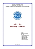
where Ψun is the scheduling metric defined in (5). The user index set I(m) , which groups users with identical quantized channel shapes, is defined as In this section, a bins-and-balls model for multiuser feed- back of quantized channel shapes is introduced. This model provides a useful tool for analyzing throughput scaling law for orthogonal beamforming in Section 5.1. In this model as illustrated in Figure 2, U balls are thrown into N + 1 bins: N small bins and one big one, whose total volume is equal to one. , 1 ≤ u ≤ U | (cid:4)su = v(m) I(m) n Some useful results are derived using the bins-and-balls model. Let the probability that a ball falls into a specific bin 1 ≤ m ≤ M, 1 ≤ n ≤ Nt. (13)
6 EURASIP Journal on Advances in Signal Processing
U balls
(cid:13)
(cid:14)
where
log , log , (20) Uo = max 3 τ1 16c τ2 4 τ1 2 τ2
· · ·
1
2
N
N + 1
and c is a constant.
Area of small bin = p
Area of big bin = 1 − N p
5. THROUGHPUT SCALING: HIGH SNR
Figure 2: The bins-and-balls model for multiuser feedback of quantized channel shapes.
(cid:6)
=
In this section, the throughput scaling law of uplink SDMA in the high SNR regime (γ (cid:10) 1) is analyzed. The expected SINR in (5) for this regime is simplified as
(cid:2)m
, (21) Ψ(α) u ρu m∈A,m /=u ρm
be equal to p for each small bin and q for the big bin, hence q = 1 − N p. The first question to ask is how many small bins are nonempty? The answer to this question is provided in the following lemma, obtained Using the Chebychev’s inequality [23]. where the superscript (α) is added to indicate the high SNR regime. Using the analytical tools discussed in Section 4, the throughput scaling laws are derived in Sections 5.1 and 5.2 for orthogonal and zero-forcing beamforming, respectively.
(cid:3)
(cid:9)(cid:29)
5.1. Throughput scaling for orthogonal beamforming Lemma 2. Denote (cid:27)p = 1−(1 − p)U . The number of nonempty small bins W satisfies
(cid:28) W ≥ N (cid:27)p −
(cid:8) N (cid:27)p − N (cid:27)p2
≥ 1 − 1 log N
(17) Pr log N .
In this section, we analyze the throughput scaling laws for orthogonal beamforming in the high SNR regime. Two cases are considered. First, both the number of users U and the quantization codebook size N are large. For this case, we de- rive an upper and a lower bounds for the throughput scaling factor as functions of U and N. Second, U is large but N is fixed. For this case, the exact throughput scaling factor in terms of U is obtained.
Next, consider clusters of Nt neighboring small bins. In Section 5.1, each cluster is related to an orthonormal vector set in the quantizer codebook for orthogonal beamforming. Each cluster is said to be nonempty if it contains no empty bins. Then, the second question to ask is how many clusters are nonempty? The answer is provided in the following corol- lary of Lemma 2. 5.1.1. U→∞ and N →∞
(cid:3)
(cid:28)
(cid:9)(cid:29)
≥ 1 − 1
Corollary 1. Denote the number of nonempty clusters of small bins as Q. Then Q satisfies
(cid:8) M (cid:27)pNt − M (cid:27)p2Nt
, Pr Q ≥ M (cid:27)pNt − log M log M (18)
where M is the total number of clusters.
or is derived as fol- lows. To avoid considering any specific scheduling algorithm in the derivation, the following assumption is made.
4.2. Uniform convergence in weak law of large numbers To derive the throughput scaling law for U→∞ and N →∞, the following approach is adopted. First, we derive an up- per bound for the throughput scaling factor of the expected throughput, which is defined in (6). To avoid confusion, the expected throughput is denoted as R(α) or where the superscript specifies the high SNR regime and the subscript indicates or- thogonal beamforming. Second, an achievable lower bound is obtained by constructing a suboptimal scheduling algo- rithm. Last, the throughput scaling law for R(α) is shown to or hold for the exact throughput. An upper bound for scaling factor of R(α)
Assumption 4. The channel power of a scheduled user is lower-bounded as:
≥
∀u ∈ A.
(cid:31)
(cid:30)
(cid:5) (cid:5) (cid:5) (cid:5)
In this section, a lemma on the uniform convergence in the weak law of large numbers [22] is obtained by generalizing [27, Lemma 4.8]. This lemma given below is useful for ana- lyzing the number of users whose channel shapes lie in one of a set of congruent disks on the surface of a hyper sphere. Such analysis will appear frequently in the subsequent throughput analysis. (22) ρu 1 log U + c
Pr (19) Lemma 3 (Gupta and Kumar). Consider U random points uniformly distributed on the surface of a unit hyper-sphere in CNt and N disks on the sphere surface that have equal volume denoted as A. Let Tn denote the number of points belong to the nth disk. For every τ1, τ2 > 0: (cid:5) (cid:5) (cid:5) − A (cid:5) ≤ τ1 > τ2 U ≥ Uo, is derived and shown in the following lemma. This assumption is justifiable under the current design criterion of maximizing throughput. Under this criterion, as U grows, the channel power of scheduled users increases but ≥ 0 and the lower bound in (22) converges to zero. Since ρu we are interested in the case of U→∞, Assumption 4 is justi- fied. Using this assumption, an upper bound for the scaling factor of R(α) or Tn U sup 1≤n≤N
Kaibin Huang et al. 7
!
Then the scheduled user set A is given as
(cid:2)u, 1 ≤ n ≤ Nt
(cid:8)
Lemma 4. In the high SNR regime and for the case of U→∞ and N →∞, the scaling factor of the expected throughput R(α) or in (6) is upper bounded as A = (27) . arg min (cid:3)) u∈I(m n
≤ 1.
(cid:8) Nt/
(23) R(α) or (cid:9)(cid:9) (log U + log N) Nt − 1 lim U→∞ B→∞ Using this scheduled algorithm, an achievable lower bound of the throughput scaling factor is obtained and shown in the following lemma.
(cid:9)(cid:9)
(cid:8)
(cid:9)(cid:9)
Lemma 5. In the high SNR regime and for the case of U→∞ and N →∞, the scaling factor of the expected throughput R(α) or in (6) is lower-bounded as
≥ 1.
(cid:8) Nt/
(cid:8) Nt − 1
(cid:8) Nt − 1
(28) R(α) or log U + 1/ log N lim U→∞ N →∞
The proof is given in Appendix C. The proof procedure involves using the bins-and-balls model and Lemma 1 in Sec- tion 4.1.
or . Let χ2
1, χ2
2, . . . , χ2 Nt
Proposition 1 implies the identical throughput scaling factors for the expected throughput R(α) or and the exact one, denoted as C(α) or , because their difference is no more than a constant. By combining Proposition 1, Lemmas 5 and 4, the main result of this section is obtained and summarized in the following theorem.
Theorem 1. In the high SNR regime and for the case of U→∞ and N →∞, the scaling law of the throughput for orthogonal beamforming is given as
(cid:9)(cid:9)
(cid:8)
(cid:9)(cid:9)
≤ 1,
⎡
⎤
The proof is given in Appendix B. Next, an achievable lower bound for the scaling factor of R(α) is obtained. The direct derivation of a scheduling al- or gorithm for maximizing the scaling factor of R(α) in (6) is or very difficult if not impossible. To overcome this difficulty, we argue that it is unnecessary to consider channel power in scheduling. In the sequel, we prove that the scheduling ne- glecting channel power leads to a reasonable lower bound of the optimum throughput scaling factor for orthogonal beamforming. The reason for the above argument is that scheduling users with largest channel power can at most in- crease the scaling factor by only O(log log U) since the largest power scales as log U [8]. Such an increment is negligible because the expected scaling factor is O(log U) as shown in Lemma 4. Thus, to achieve the optimum throughput scaling, using minimum quantization errors {(cid:2)u} as the scheduling criterion suffices. In the high SNR regime that is interference limited, such a criterion minimizes interference caused by quantization errors. The use of only quantization errors as the scheduling criterion leads to the following lower bound for R(α) denote a sequence of chi-squared random variables representing the channel power of sched- uled users. From (6) and (21),
(cid:8) Nt/
(cid:8) Nt − 1
(cid:30)
(cid:31)
Nt(cid:2)
(cid:6)
C(α) or (cid:8) log U + log N Nt/ Nt − 1 lim U→∞ N →∞
(cid:8)
(cid:9)(cid:9)
(cid:8)
(cid:9)(cid:9)
⎥ ⎥ ⎥ ⎦
≥ 1.
⎢ ⎢ ⎢ ⎣ max 1≤m≤M
(cid:2)uk
n=1
k
(cid:8) 1/
(cid:8) Nt/
(cid:30)
(cid:31)(cid:10)
(cid:7)
Nt(cid:2)
(cid:6)
log 1 + Ror ≥ E χ2 n Nt k=1,k /=nχ2 C(α) or log U + log N Nt − 1 Nt − 1 lim U→∞ N →∞ max uk ∈I(m) k k=1,...,Nt (29)
≥ E
(cid:2)u
n=1
k
≥ NtE
log 1+ A few remarks are in order. χ2 n Nt k=1,k /=n χ2 kmin u∈I(m) max 1≤m≤M (cid:7)
(cid:31)(cid:10)
(cid:6)
× log
max 1≤m≤M (cid:30)
(cid:2)u
k
n
Nt k=1,k /=nχ2
(cid:7)
(cid:30)
1+
(cid:6)
χ2 n min u∈I(m) (cid:31)(cid:10)
= NtE
(cid:2)(cid:3)
k
log 1 + , max1≤n≤Nt χ2 n N k=1, k /=nχ2 (i) The bounds in (29) agree on that the throughput scal- ing factor with respect to U is (Nt/(Nt − 1)) log U. (ii) The lower and the upper bounds in (29) differ by Nt times in the throughput scaling factor with respect to N. The smaller scaling factor in the constructive lower bound is due to the use of a suboptimal scheduling algorithm. The design of a scheduling algorithm for achieving the upper bound for the scaling factor in (29) is a topic for future investigation. (24)
where
(cid:2)u.
(cid:2)(cid:3) = min 1≤m≤M
(iii) No feedback of channel power is required for achiev- ing the lower bound for the throughput scaling factor in (29), because scheduling is independent of channel power. (25) max 1≤n≤Nt min u∈I(m) n 5.1.2. U→∞ and N fixed
(cid:30)
(cid:31)
A scheduling algorithm directly follows from the throughput lower bound in (24). Define
(cid:2)u
(26) . m(cid:3) = arg min 1≤m≤M In this section, the throughput scaling law for orthogonal beamforming is analyzed for the high SNR regime and the case where the codebook size N is fixed and the number of users U→∞. max 1≤n≤Nt min u∈I(m) k
8 EURASIP Journal on Advances in Signal Processing
5.2. Throughput scaling for zero-forcing beamforming
The upper bound of the throughput scaling factor is shown in the following lemma. The proof can be easily mod- ified from that for Lemma 4 by substituting lim U→∞ log N/ log U = 0.
zf and Cα zf .
(cid:9)(cid:9)
In this section, the scaling law for zero-forcing beamforming in the high SNR regime is analyzed. Two cases are considered: (1) U→∞ and N →∞ and (2) U→∞ and N is fixed, which are jointly analyzed due to their similarity in analysis. De- note the expected and the exact throughput for zero-forcing beamforming in the high SNR regime as Rα Lemma 6. In the high SNR regime and with N fixed, the throughput scaling factor for orthogonal beamforming is upper- bounded as
≤ 1.
(cid:8) Nt/
≤ 1,
(30) lim U→∞ log U R(α) or (cid:8) Nt − 1 The upper bounds of the throughput scaling factor for orthogonal beamforming in Lemmas 4 and 6 can be shown to hold for zero-forcing beamforming by trivial modifica- tions of the proofs. Thus,
(cid:8) Nt/
(cid:8) Nt − 1
n
(cid:9)(cid:9)
≤ 1.
R(α) (cid:9)(cid:9) zf (log U + log N) lim U→∞ N →∞ (34)
(cid:8) Nt/
n
lim U→∞ log U R(α) (cid:8) zf Nt − 1
(cid:7)
(cid:30)
(cid:31)(cid:10)
(cid:24)
(cid:25)
(cid:5) (cid:5)q†
Next, the equality in (30) is shown to hold using the fol- lowing scheduling algorithm. First, among users belonging to the index set I(m) , the one with the smallest quantiza- tion error is selected. Second, among the selected users cor- responding to the index sets {I(m) n }, an arbitrary set of users with orthogonal quantized channel shapes are scheduled and these orthogonal vectors are applied as their beamforming vectors. Using this scheduling algorithm, the index set of scheduled users can be written as A = {arg min u∈I(m) (cid:2)u, 1 ≤ n ≤ Nt}. Based on the above scheduling algorithm and from (6), the expected throughput is bounded as The above upper bounds for the throughput scaling fac- tor of zero forcing beamforming can be achieved using the following scheduling algorithm. Consider an arbitrary basis of CNt , denoted as {q1, q2, . . . , qNt }. Using this basis, we de- fine the following index sets:
(cid:5) (cid:5)2 ≤ τo
n
(cid:6)
≥ NtE
N
(cid:2)u
k
(35) 1 ≤ u ≤ U | 1− 1 ≤ k ≤ Nt, log 1 + (31) . R(α) or χ2 n k=1,k /=nχ2 k min u∈I(m)
Using the above throughput lower bound and Lemma 6, the following lemma is proved.
(cid:13)
(cid:14)
Jk = (cid:4)su where τo = sin2((π/4) − (ϕo/2)) = (1 + sin(ϕo))/2 and (cid:4)su is the quantized channel shape. The purpose of these index sets is to select users who satisfy the zero-forcing beamforming constraint in (14). Among the users in each of the index sets {Jk}, the one with the smallest quantization error is sched- uled. In other words, the index set of the scheduled users is Lemma 7. The upper bound of the throughput scaling factor in (30) is achievable:
(cid:2)u, 1 ≤ k ≤ Nt
(cid:9)(cid:9)
= 1.
(cid:8) Nt/
A = (36) . arg min u∈Jk (32) lim U→∞ log U R(α) or (cid:8) Nt − 1
(cid:7)
(cid:30)
(cid:31)(cid:10)
(cid:6)
The beamforming vectors of the scheduled users are com- puted from their quantized channel shapes using the zero- forcing method. From the above, scheduling algorithm re- sults in the following throughput lower bound: The proof is given in Appendix D. This proof makes use of the theory of uniform convergence in the weak law of large numbers as discussed in Section 4.2.
≥ NtE
N
(cid:2)u
log 1 + (37) . R(α) zf By combining Lemma 7 and Proposition 1, the main re- sult of this section is obtained and summarized in the follow- ing theorem. χ2 n k=1,k /=nχ2 kmin u∈Jk
Using the above throughput lower bound, we prove the following theorem. Theorem 2. In the high SNR regime (γ (cid:10) 1) and with a fixed codebook size N, the throughput scaling law for orthog- onal beamforming is
(cid:9)(cid:9)
= 1.
(cid:8) Nt/
Theorem 3. In the high SNR regime, the throughput scaling law for zero-forcing beamforming is given as follows. (33) lim U→∞ (1) For U→∞, N →∞, log U C(α) or (cid:8) Nt − 1
(cid:9)(cid:9)
(cid:9)(cid:9)
= 1.
(cid:8) Nt/
(cid:8) Nt − 1
(cid:8) Nt − 1
(cid:8)
(cid:8)
(cid:9)(cid:9)
Two remarks are given. log N C(α) (cid:8) zf log U + Nt/ lim U→∞ N →∞ (38) (i) The current throughput scaling factor is identical to the first terms of the bounds in (29) corresponding to the case of N →∞. (2) For U→∞, N fixed
= 1.
(39) log U Nt/ C(α) zf Nt − 1 (ii) For Nt ≥ 3, the linear scaling factor in (33), namely, Nt/(Nt − 1), is smaller than Nt, which is the number of available spatial degrees of freedoms. This indicates the loss in multiplexing gain for Nt ≥ 3. lim U→∞ N →∞
(cid:5) T (m)
n ⊂ I(m)
n
(cid:5) T (m) n
Kaibin Huang et al. 9
The proof is given in Appendix E. The proof uses the uni- form convergence in the weak law of large numbers. As be- fore, Proposition 1 is applied to equate the scaling laws be- tween the expected and the exact throughput.
and a scalar Uβ := exp (−dmin /4). Then for all U ≥ Uβ. From each set , the user with the maximum channel power is selected. Next, among the selected users, up to Nt users are scheduled using the criterion of maximizing throughput. Using this scheduling algorithm and from (12), a lower-bound of the throughput is obtained as
(cid:7)
(cid:30)
(cid:31)(cid:10)
Nt(cid:2)
n
(cid:6)
≥E
Ror
n=1
k
log 1+ A few remarks are in order. (i) For U→∞, N →∞, the throughput scaling factor for zero-forcing beamforming upper bounds that for or- thogonal beamforming (cf. (29)). Note that this does not imply the former is larger since the achievability of the same scaling factor for orthogonal beamforming is unknown. 1+γ max 1≤m≤M γmaxu∈T (m) Nt k=1, k/=umaxu(cid:5)∈T (m)
(cid:30)
(cid:7)
(cid:31)(cid:10)
Nt(cid:2)
n
(cid:6)
≥E
ρu ρu(cid:5) (1/log U) U ≥ Uβ
n=1
k
log 1 + 1 + γ (ii) The same scaling laws as in (3) have been also proved for downlink SDMA with limited feedback [6]. They are derived using a different approach based on the extreme value theory, though. This similarity demon- strates uplink-downlink duality. γmax u∈T (m) ρu Nt ρu(cid:5) (1/ log U) k=1,k /=umax u(cid:5)∈T (m) U ≥ Uβ. (42)
(iii) As for orthogonal beamforming, the scheduling algo- rithm, which achieves the above scaling laws for zero- forcing beamforming, requires no feedback of channel power.
Using the above lower bound, we prove the following theo- rem. 6. THROUGHPUT SCALING: NORMAL SNR
Theorem 4. In the normal SNR regime, the scaling law for or- thogonal beamforming is
= 1.
(43) lim U→∞ Cor Nt log log U
In this section, the throughput scaling law for uplink SDMA in the normal SNR regime is analyzed. In this regime, nei- ther the noise nor the interference dominates, thus the SINR and scheduling metric are given, respectively, in (4) and (5). The throughput scaling law for orthogonal beamforming and zero-forcing beamforming are analyzed separately in Sec- tions 6.1 and 6.2.
6.1. Orthogonal beamforming The proof is given in Appendix F. Again, the proof relies on the uniform convergence in the weak law of large num- bers. A few remarks are in order.
In this section, the throughput scaling factor for orthogonal beamforming is obtained by deriving an upper bound and an achievable lower bound of this factor.
(i) The throughput in the normal SNR regime scales as log log U but that in the high SNR regime increases as log U. Therefore, the throughput scaling rate is much higher in the high SNR regime than in the normal SNR regime. The upper bound of the scaling factor is given in the fol- lowing lemma. This upper bound also holds for the low SNR regime and the zero-forcing beamforming. (ii) The scaling law in Theorem 4 shows the full multiplex- ing gain.
Lemma 8. For both the normal and low SNR regimes, the throughput scaling factors for both orthogonal and zero-forcing beamforming are upper-bounded as
≤ 1.
(iii) Besides quantized channel shapes, feedback of both channel power and quantization errors from users are required. (40) lim U→∞ Ror/zf Nt log log U 6.2. Zero-forcing beamforming
(cid:31)
(cid:30)
The proof is similar to that for Lemma 4 and hence omit- ted. In the proof, the upper bound of the throughput scaling factor in (40) is derived by omitting interference. This im- plies that reducing interference by increasing the codebook size N has no effect on this upper bound. Thus it is unnec- essary to consider the case of N →∞ in the analysis for the normal SNR regime. The scheduling algorithm for achieving the equality in This section focuses on the throughput scaling law for zero- forcing beamforming in the normal SNR regime. A schedul- ing algorithm for achieving the scaling upper bound in Lemma 8 is constructed as follows. Define the index sets, {Tn}N n=1, similar to (41) but based on the RVQ codebook for zero-forcing beamforming (cf. Section 3.3.2). Next, define a new index set
(cid:30)
N"
(cid:5) T (m)
(40) is provided as follows. Define the user index sets (cid:31)!
n =
n
n=1
, (44) (41) Lk = Jk ∩ Tn 1 ≤ k ≤ Nt, 1 ≤ u ≤ U | su ∈ B(m) 1 (log U)Nt −1
10 EURASIP Journal on Advances in Signal Processing
!
Theorem 6. In the low SNR regime, the scaling law of uplink SDMA with orthogonal beamforming is given as where Jk is given in (35). From users in each of the sets {Lk}, the one with the maximum channel power is sched- uled. Thus, the index set of scheduled users is given as
= 1.
(β) C or Nt log log U
(49) lim U→∞ A = (45) . ρu, 1 ≤ k ≤ Nt max u∈Lk
Using the above scheduling algorithm, we obtain the follow- ing theorem by proving the achievability of the throughput- scaling upper bound in Lemma 8. The proof is similar to that for Theorem 4. Specifically, the proof uses the result of the extreme value theory in (B.6) and Lemma 3 of the uniform convergence in the weak law of large numbers. The details of the proof are omitted.
Theorem 5. In the normal SNR regime, the scaling law for zero-forcing beamforming is
= 1.
(46) lim U→∞ Czf Nt log log U Comparing Theorems 4 and 6, the scaling laws in the normal and the low SNR regimes are identical. The intuition is that the interference power decreases continuously with U. Thus, for a large U, both the low and normal SNR regimes become noise limited, resulting in the same throughput scal- ing laws.
7.2. Zero-forcing beamforming
The proof is given in Appendix G. The proof involves re- peated applications of Lemma 3, which show the uniform convergence of the numbers of users in the index sets {Tn} and Jn defined (35), respectively.
Comparing Theorems 4 and 5, the same scaling law holds for both orthogonal and zero-forcing beamforming in the normal SNR regime. Furthermore, this scaling law is identical to that for downlink SDMA with limited feedback [6, 8, 17].
!
7. THROUGHPUT SCALING: LOW SNR As in the last section, the derivation of the throughput scaling law for zero-forcing beamforming in the low SNR regime re- lies on the use of a specific scheduling for achieving the scal- ing upper bound in Lemma 8. This scheduling algorithm is simplified from that in Section 6.2 as follows. For the current algorithm, the scheduled users are selected from the index sets {Jk} in (35) rather than {Lk} as in Section 6.2. Conse- quently, the index set of scheduled users is A = (50) . ρu, 1 ≤ k ≤ Nt max u∈Lk
Using the above scheduling algorithm, we prove the follow- ing theorem. In this section, the analysis of the throughput scaling law for uplink SDMA focuses on the lower SNR regime where chan- nel noise is dominant. In this regime, the expected SINR in (5), denoted as Ψ(β), reduces to γ ρu. The following analysis is presented in Sections 7.1 and 7.2, which correspond, respec- tively, to orthogonal and zero-forcing beamforming.
Theorem 7. In the low SNR regime, the scaling law for zero- forcing beamforming is 7.1. Orthogonal beamforming
= 1.
(β) or and C
(51) lim U→∞ Czf Nt log log U
In the lower SNR regime, the throughput scaling law for or- thogonal beamforming is obtained by achieving the upper bound for the throughput scaling factor in Lemma 8 using a specific scheduling algorithm. Denote the expected and exact throughput as R
(β) or , respectively. A suitable scheduling algorithm can be modified from that in Section 6.1 by replacing the index sets in (41) with the following ones:
(cid:24)
(cid:8)(cid:8)
The proof is a simplified version of that for Theorem 7 due to the similarity in scheduling algorithms. Unlike the previous proof, the current proof requires only one-time ap- plication of Lemma 3. Similar remarks for Theorem 6 are also applicable here.
Nt −1(cid:9)(cid:25)
=
n
(cid:9) , dmin /4 1 ≤ m ≤ M, 1 ≤ n ≤ Nt.
n ∩ ˇT (m(cid:5)) ˇT (m)
n(cid:5)
= ∅ for all (m, n) /= (m(cid:5), n(cid:5)). Note that The modified scheduling algorithm leads to the following throughput lower bound: (cid:7)
(cid:31)(cid:10)
(cid:30)
8. NUMERICAL RESULTS 1 ≤ u ≤ U | su ∈ B(m) ˇT (m) n (47)
(β) or ≥ NtE R
log (48) . ρu 1 + γ max u∈ ˇT (m) n
Using the above throughput lower bound, the through- put scaling law is obtained and summarized in the following theorem. In this section, based on simulation, orthogonal and zero- forcing beamforming are compared in terms of uplink SDMA throughput for an increasing number of users U. Such a comparison is to evaluate the throughput difference between orthogonal and zero-forcing beamforming in the practical regime of U. Note that the throughput scaling laws derived in previous sections indicate the same slopes for the throughput versus U curves for both beamforming methods in the asymptotic regime of U. Furthermore, uplink SDMA with limited feedback is compared with uplink channel- aware random access proposed in [28], which requires no CSI feedback.
4.5
16
15
4
14
3.5
13
) z H
) z H
12
3
/ s / b (
/ s / b (
11
2.5
10
t u p h g u o r h T
9
t u p h g u o r h T
2
8
1.5
7
1
6
0
20
40
100
120
140 150
80
0
20
40
100
120
140 150
80
60 Number of users
60 Number of users
Orthogonal (0 dB) ZF (0 dB)
Orthogonal (−5 dB) ZF (−5 dB)
Orthogonal (30 dB) Orthogonal (20 dB)
ZF (30 dB) ZF (20 dB)
(a) High SNR
(b) Low SNR
Kaibin Huang et al. 11
Figure 3: Throughput comparisons between orthogonal and zero-forcing beamforming for uplink SDMA in (a) the high SNR regime and (b) the low SNR regime. The number of antennas at the base station is Nt = 2 and the quantizer codebook size is N = 8. The plotted values in brackets specify the SNR values in dB.
6
5
) z H
4
/ s / b (
3
t u p h g u o r h T
2
1
0
50
100
150
Number of users
SDMA (ZF) SDMA (orthogonal) Random access (number of scheduled users = 1) Random scheduling (number of scheduled users = 1) Random scheduling (number of scheduled users = 2)
optimum throughput scaling in Sections 5 and 7. For zero- forcing beamforming, the scheduling algorithms are modi- fied from that proposed in [6] by using the above criterions in greedy-search scheduling. For orthogonal beamforming, the scheduling algorithms are identical to those proposed in Sections 5.1 and 7.1. The throughput of orthogonal and zero-forcing beamforming are compared in Figure 3 for an increasing number of users U. For this comparison, the num- ber of antennas is Nt = 2, the quantizer codebook size is N = 8, and the SNRs are {−5, 0} dB for the low SNR regime and {20, 30} dB for the high SNR regime. Several observations are made from Figure 3. First, as shown Figure 3(a) for the high SNR regime, orthogonal beamforming provides higher (smaller) throughput than zero-forcing beamforming if the number of users is large (small). The crossing point between the curves for orthogonal and zero-forcing beamforming is at U = 20 for SNR = 20 dB and at U = 28 for SNR = 30 dB. Second, from Figure 3(b) for the low SNR regime, orthog- onal beamforming always achieves higher throughput than zero-forcing beamforming. Note that for U→∞, the curves for orthogonal and zero-forcing beamforming have identical slops according to the throughput scaling laws.
Figure 4: Throughput comparisons between uplink SDMA with limited feedback, SDMA with random scheduling, and uplink ran- dom access in [28]. The number of antennas at the base station is Nt = 2; the quantizer codebook size is N = 8; the SNR = 5 dB.
In Figure 4, the throughput of uplink SDMA is compared with that of SDMA with random scheduling and uplink ran- dom access [28], both of which require no CSI feedback. For SDMA with random scheduling, a random set of users is scheduled and their beamformers are columns of a random orthonormal basis. Note that with single-scheduled users, SDMA with random scheduling reduces to TDMA. For up- link random access, transmitting users are selected distribu- tively using a channel power threshold, which increases with the total number of users [28]. For fair comparison, the up- link random access design originally proposed in [28] for Orthogonal and zero-forcing beamforming are com- pared for both the high and the low SNR regimes. For sim- ulation, the scheduling criterion is minimum quantization error in the high SNR regime and maximum channel power in the low SNR regime. These criteria are shown to achieve
12 EURASIP Journal on Advances in Signal Processing
APPENDICES
A. PROOF OF PROPOSITION 1
(cid:9)
(cid:5) (cid:8) (cid:5) ≤ ∠
Using the triangular inequality, |∠(vu, (cid:4)su) − ∠(su, (cid:4)su)| ≤ ∠(vu, su) ≤ ∠(vu, (cid:4)su) + ∠(su, (cid:4)su). By definitions of ϕu and θu, the above expression can be rewritten as
− θu
(cid:5) (cid:5)ϕu
≤ ϕu + θu.
(A.1) vu, su
(cid:31)(cid:10)
(cid:7)
(cid:30)
(cid:9)(cid:9)
(cid:2)
From the given condition ϕu + θu ≤ ϕ0 + θ0 < π/2 and (A.1), cos(∠(vu, su)) ≥ cos(ϕ0 + θ0). Using this inequality, (9), and (4), then
(cid:8) (cid:8) ∠ vu, su
(cid:30)
(cid:2)mβm,u (cid:31)(cid:10) (cid:9)
u∈A (cid:7) (cid:2)
γ ρucos2 (cid:6) log 1 + C = E 1 + γ
(cid:2)m
u∈A
(a) ≥ E (cid:7)
m∈A,m /=u ρm (cid:8) ϕ0 + θ0 m∈A,m /=u ρm (cid:9)(cid:9)
γ ρucos2 (cid:6) log 1 + 1 + γ
≥ E
|A| log
(cid:8) ϕ0 + θ0
(cid:8) cos2 (cid:30)
(cid:31)(cid:10)
(cid:2)
SISO channels is modified to allow transmit beamforming at each user who has Nt antennas. For uplink SDMA with lim- ited feedback, the scheduling algorithms used in the previous comparison for the low SNR regime are applied. The simula- tion parameters are SNR = 5 dB, Nt = 2, and N = 8. Several observations are made from Figure 4. First, the throughput for uplink SDMA is much higher than that of SDMA with random scheduling and uplink random access. The through- put gains of uplink SDMA result from scheduling at the base station and the support of Nt simultaneous users. Second, the throughput of SDMA with random scheduling and up- link random access is insensitive to changes on the number of users U for the following reasons. Without giving prefer- ence to users with large channel power, random scheduling is incapable of exploiting multiuser diversity. Next, uplink ran- dom access achieves the throughput scaling of log log U but such a function grows extremely slowly with U. In summary, uplink SDMA outperforms SDMA with random scheduling and uplink random access in [28] by a large margin at the expense of finite-rate feedback from each user. Note that it is possible to schedule feedback users so as to constraint the total feedback overhead for uplink SDMA by following an approach similar to those proposed in [18, 29]. (A.2)
(cid:6)
(cid:2)m
(cid:8)
≤ 1. Next, an upper bound is obtained
9. CONCLUSION + 1 + γ (cid:9)(cid:9) γ ρu m∈A,m /=u ρm + R 1 + (cid:8) ϕ0 + θ0 (cid:9)(cid:9) cos2 + R. log u∈A (cid:8) = |A| log cos2 (cid:8) ≥ log ϕ0 + θ0
(cid:7)
(cid:30)
(cid:31)(cid:10)
(cid:2)
(cid:6)
For (a), note that βm,n for the throughput C as follows:
(cid:2)m
m∈A,m /=u ρm
u∈A
⎡
(cid:2)
⎢ ⎣
⎟ ⎠
≤E
log C ≤E 1+ ⎛ ⎛ γ ρu 1+min m∈A,m /=uβm,uγ ⎞ &
⎜ ⎜ ⎝1 ⎝
u∈A
⎛
⎞ ⎞ ⎞ ⎤
(cid:2)
log In this paper, the scaling law of uplink SDMA with limited feedback is analyzed for different SNR regimes and both or- thogonal and zero-forcing beamforming. In the high SNR regime and for orthogonal beamforming, for an increasing quantizer codebook size, the throughput scales logarithmi- cally with both the number of users and the codebook size; for a fixed codebook size, the throughput scales logarithmi- cally only with the codebook size. For both cases, the linear scaling factor is smaller than the number of antennas, indi- cating the loss in spatial multiplexing gain. Similar results are obtained for zero-forcing beamforming. In the normal SNR regime, for both orthogonal zero-forcing beamforming, the throughput is found to scale double logarithmically with the number of users and linearly with the number of antennas. The same results are obtained for the low SNR regime. βm,u ⎛ min m∈A m /=u &
⎟ ⎟ ⎟ ⎥ ⎟ ⎟ ⎟ ⎥ (cid:2)m ⎦ ⎠ ⎠ ⎠
⎜ ⎜ ⎝γ ρu
⎜ ⎜ ⎝min m∈A m /=u
m∈A m /=u
(cid:31)(cid:10)
(cid:7)
(cid:30)
(cid:2)
(cid:6)
≤E
+ ρm βm,uγ βm,u +min m∈A m /=u
(cid:2)m
u∈A
+
* + |A|E
log 1 + 1 + γ Simulation results suggest that orthogonal and zero- forcing beamforming achieve different uplink throughput in nonasymptotic regimes even though they may follow the same throughput scaling laws asymptotically. For a small SNR or a large SNR coupled with many users, orthogonal beamforming outperforms zero-forcing beamforming. The reverse is true for a large SNR and a small number of users. γ ρu m∈A,m /=u ρm ,-
(a)
βm,u
− log min m∈A,m /=u (cid:9) (cid:8) |A| − 1 Nt − 1 (cid:8)
≤ R + |A| log (cid:11)
(cid:12) , + 1
+ 1
≤ R +
(cid:9) Nt − 1
log Nt Nt − 1 (A.3)
where the inequality (a) is obtained by applying Lemma 1. Combining (A.2) and (A.3) gives the desired result. The analysis in this paper opens several interesting top- ics for future investigation. First, how to design a scheduling algorithm for uplink SDMA with orthogonal beamforming that achieves the optimum throughput scaling factor in the high SNR regime? Second, how to design scheduling algo- rithms for maximizing uplink SDMA throughput in practi- cal regimes? Note that the scheduling algorithms discussed in this paper only ensure the asymptotic throughput scal- ing. Third, how to select feedback users for reducing the sum feedback rate along the vein of [18, 29]? Last, what is the rel- ative efficiency of limited and analog feedback?
Kaibin Huang et al. 13
B. PROOF OF LEMMA 4
(cid:7)
(cid:30)
Nt(cid:2)
(a) ≤ E
(cid:2)u(cid:5)
n=1
k
(cid:31)(cid:10)
n
(cid:2)u(cid:5)
k
(cid:31)
(cid:7)
(cid:30)
Nt(cid:2)
≤ E
From (6) and given Assumption 4, The equality (a) is a property of the quantization for orthog- onal beamforming [17] where {βu,n } are i.i.d. delta random variables, (b) is obtained by applying Lemma 1. The desired result follows from (B.8) and (B.7). log R max 1≤m≤M 1 max u(cid:5)∈I(m) C. PROOF OF LEMMA 5 ρu + (log U + c)max u∈I(m) min u(cid:5)∈I(m)
n=1
(cid:31)(cid:10)!
− log
(cid:2)u(cid:5)
log ρu The proof is divided according to three cases: N = o(U), N = Θ(U), and N = O(U). Only the proof for the case N = o(U) is presented below and those for other two cases are omitted due to their similarity. max 1≤m≤M 1 + (log U + c) max u∈I(m) n (cid:30)
,-
+
* (b) ≤ NtE
min u(cid:5)∈I(m) k
− NtE
(cid:2)u(cid:5)
(cid:24)
(cid:25)
(cid:5) (cid:5)s†v(m)
n
+
,-
(cid:5) (cid:5)2 ≤ A1/(Nt −1) 1 ≤ m ≤ M, 1 ≤ n ≤ Nt,
ρu log (cid:7) 1 + (log U + c) max 1≤u≤U (cid:31)(cid:10) (cid:30) To begin, a bins-and-balls model is constructed for mul- tiuser feedback of quantized channel shapes as follows. In this model, the U balls of the channel shapes of U users, which are i.i.d. points, uniformly distributed on the surface of the unit hyper sphere. The small bins (cf. Section 4.1) are N congruent disks on the unit hyper-sphere as defined be- low: log min 1≤m≤M min u(cid:5)∈I(m) k s ∈ CNt | (cid:2)s(cid:2)2 = 1, 1 − , (A) = (B.4) B(m) n
− Π.
* = NtE
k
(cid:2)u(cid:5) ≤ 1). The in- The inequality (a) follows from (max u(cid:5)∈I(m) equality (b) is obtained by moving the “max” operator in (B.4) into the summation term. The definition of Π in (B.5) is obvious.
log (B.5) ρu (C.9) 1 + (log U + c) max 1≤u≤U
n
(cid:9)(cid:25)
,
+
,
=
(cid:8) U −1
n
− log U
(cid:5) (cid:5) (cid:5) (cid:5) < O(log log U)
+(cid:5) (cid:5) (cid:5) (cid:5) max 1≤u≤U
n
n = |T (m) |. De- n , 1 ≤ n ≤ Nt}.
(cid:24)
(cid:11)
(cid:12)(cid:25)
(cid:25)
(cid:24)
+
,-
n
×
The following result is well known from extreme value is specified by the following index set: theory (see, e.g., [8, Equation (A10)]): where A = 1/U is the disk volume. Note that the volume of the big bin is 1−N/U. Following this definition, each disk (or small bin) is centered at a code vector in the codebook F (cf. Section 3.3.1) and has a volume 1/U. The set of balls inside the small bin B(m) (cid:24) (C.10) 1 ≤ u ≤ U | B(m) . T (m) n Pr > 1 − O . ρu 1 log U (B.6) is T (m) n From (B.5) and (B.6), Therefore, the number of balls in B(m) fine the mth cluster of small bins as {B(m) Furthermore, define the index set for nonempty clusters: log U + O(log log U) R ≤ Nt log Q = (C.11) 1 ≤ m ≤ M : T (m) . /= ∅ ∀1 ≤ n ≤ Nt
* 1 − O (cid:7)
(cid:31)(cid:10)
+
,
U(cid:2)
1 + (log U + c) 1 log U (cid:30)
u=1
(cid:24)
(cid:12)(cid:25)
log O + Π 1 + (log U + c) + NtE ρu
,
+
⊂ I(m)
n
n
n
× O
1 log U (cid:11) 1 + (log U + c)UE ρu ), where T (m)
,
n
(cid:12) O
≤ O(log log U) + Nt log 1 log U (cid:11) 1 + (log U + c)UNt
n
n
.
+ Π = O(log log U) + Thus the number of nonempty clusters is Q = |Q|. The above bins-and-balls model allows us to apply Lemma 1 for characterizing Q. Specifically, Q satisfies (18) with p = 1/U. Next, we derive the probability that a small bin lies inside and are defined in (C.10) and (13), respectively. This prob- /= ∅ is given in + Π. a Voronoi cell, namely, Pr (T (m) I(m) n ability conditioned on a nonempty bin T (m) the following lemma. + Nt log 1 log U (B.7) and I(m) have the following Lemma 9. The index sets T (m) relationship:
1≤m≤M
+
,M−1
≥
(cid:9) /= ∅
,-
+
(cid:8) T (m) n
⊂ I(m) n
| T (m) n
− log
* Π ≤ NtE
(cid:2)u
+
,-
=
Last, a close-form expression is derived for Π defined in I(m) n ∈ {u | 1 ≤ u ≤ U}, Π is upper- (B.5). Since bounded as Pr . 1 − Nt4Nt −1 U (C.12) min 1≤u≤U
* (a)= NtE
−1/(Nt −1) N t
− log *
2
(b)= Nt
|
n
n
(B.8) min 1≤u≤U min 1≤n≤M βu,n - a T (m) n . log (MU) + log Nt + ∅, is 1−|v†v(m) Proof. Define Given condition for u ∈ T (m) U −1/(Nt −1). sufficient ≥sin2(2θ) sin2θ /= n ⇒ u ∈I(m) 1 Nt − 1 Nt − 1
14 EURASIP Journal on Advances in Signal Processing
⎞
⎛
⎤
⎡
(cid:9)
(cid:9) /= ∅ (cid:5) (cid:5)2 ≥ sin2(2θ) ∀v ∈ F , v /= v(m)
n
n
N(cid:2)
(cid:8)
(cid:9)(cid:12)
(cid:12)
(cid:12)M−1
, whose proof is straightforward for all v ∈ F and v /= v(m) n and hence omitted. Using this sufficient condition, Using the above results, the lower bound of the scaling is readily obtained as factor of the expected throughput R(α) or follows. From (24), Pr
⎢ ⎢ ⎣log
⎟ ⎟ ⎠
⎜ ⎜ ⎝
(cid:11) ≥ NtE
− NtE
⎥ (cid:11) ⎥ ⎦ − NtE
(cid:8) T (m) | T (m) ⊂ I(m) n n n (cid:5) (cid:8) (cid:5)v†v(m) 1 − ≥ Pr (cid:11) (a)= 1 − Nt(sin 2θ)2(Nt −1)
k=1 k /=n
(cid:9)(Nt −1)(cid:12)M−1
(cid:12)
≥
log log (cid:2)(cid:3) R(α) or χ2 n χ2 k
(cid:8) 4sin2θ
(cid:11) 1 − Nt
(cid:11) = O(1) − NtE
(cid:12)
(cid:8)
(cid:9)
(cid:27)(cid:2) = (cid:2)(cid:3)
, (C.13)
(cid:12)(cid:9)
(cid:9)
log (cid:2)(cid:3) (cid:11) (a) (cid:2)(cid:3) ≥ O(1) − Nt log E ≥ O(1) − Nt log E[(cid:27)(cid:2)] Pr
(cid:8) (cid:27)(cid:2) = (cid:2)(cid:3)
(b) ≥ O(1)−Nt log
(c) ≥ O(1) − Nt log
where (a) is a property of the quantization codebook for or- thogonal beamforming, which consists of M randomly gen- erated orthonormal sets [17]. The desired result follows from the last equation and the definition of sin θ. Pr
n
(cid:11) (cid:8) U −1/(Nt −1)E Q−1/Nt(Nt −1) 1 U −1/(Nt −1) (cid:3)
/
0−1/Nt(Nt −1)2
(cid:3)
× (cid:28)
(cid:2)u.
(cid:29) log Mvar(Q)
(cid:27)(cid:2) = min 1≤m≤M
× Pr ((cid:2)(cid:3) = (cid:27)(cid:2)) Pr (cid:7)+
-
(d) ≥ O(1)+
+
,M−1+
×
To use the result based on the bins-and-balls model, the in (25) with : following variable is defined by replacing I(m) T (m) n M p− log M var(Q) (C.14) max 1≤n≤Nt min u∈T (m) k Q ≥ M p − , A useful result is provided in the following lemma. log U + log M+O(1) Nt Nt − 1 Lemma 10. The mean of (cid:27)(cid:2) in (C.14) is upper-bounded as
(cid:12) ,
1 − 1 1 Nt − 1 , .
(cid:11) Q−1/Nt(Nt −1) E[ (cid:27)(cid:2) ] ≤ U −1/(Nt −1)E
(C.15) 1 − Nt4Nt −1 U log M (C.20) where Q := |Q| and Q is defined in (C.11).
(cid:7)
(cid:10)
Proof. From (C.14) and the definition of Q in (C.11),
(cid:2)u
n
E[ (cid:27)(cid:2) ] ≤ E (C.16) . min m∈Q max 1≤n≤Nt min u∈T (m) k The inequality (a) is the result of the Jensen’s inequality; (b) is obtained by using Lemma 10; (c) results from Lemma 1. The inequality (d) is obtained using Lemma 9, (25), and (C.14). The desired result in Lemma 5 follows from the last inequal- ity.
n
∼= U −1/(Nt −1)β, where β is a beta random For u ∈ T (m) variable (cf. Lemma 1) and ∼= denotes the equivalence in dis- tribution. Therefore, from (C.16) and the definition of T (m) in (C.10), then
0
(cid:2)u | u ∈ T (m)
k
, (cid:2)u D. PROOF OF LEMMA 7
0
min m∈Q max 1≤n≤Nt (C.17)
/ E[ (cid:27)(cid:2) ] ≤ E / = E
. U −1/(Nt −1)βm,n min m∈Q max 1≤n≤Nt
(cid:28)
(cid:29)
n
≤ (cid:2)0
= (cid:2)(Nt −1)N1 0
Next, a close-form expression is derived for the lower bound in (C.17). Since The idea for proof is summarized as follows. Consider a set of disks as defined in (C.9). A user is said to be in a disk if his/her channel shape belongs to the disk. First, the uniform convergence of the numbers of users in the N disks is shown using Lemma 3. Second, for a large number of users, a disk is shown to lie inside a corresponding Voronoi cell. With this result, considering only users in the disks rather than all re- sults in a throughput lower bound that is tight for a large number of users. Consider a set of N disks {B(m) , (C.18) Pr βm,n max 1≤n≤N1
n
(cid:13)
+
,(cid:14)
=
(1/ log U)} as defined in (C.9), each has a volume of 1/ log U. A corollary of Lemma 3 is provided as follows. Define the index set of the users in the disk B(m) (1/ log U):
≥ (cid:2)0) = (1 − we have Pr (min 1≤m≤N2 max 1≤n≤N1 βm,n (cid:2)(Nt −1)N1 )N2. Using the above CDF and following the simi- 0 lar procedure in the proof of Lemma 1 (cf. [21]), we obtain that
(cid:4)T (m) n
n
0
, 1 ≤ u ≤ U | su ∈ B(m) 1 log U (D.21) 1 ≤ m ≤ M, 1 ≤ n ≤ Nt. (C.19)
/ E
(cid:11) Q−1/Nt(Nt −1) = E
(cid:12) .
βm,n min m∈Q max 1≤n≤Nt
The desired result follows from the last equation and (C.17). The following corollary follows from Lemma 3 by substitut- ing A = 1/ log U and τ1 = τ2 = 1/ log U.
n)] = O(1) and by applying Jensen’s inequality,
Kaibin Huang et al. 15
⎞
⎛
(cid:10)
+
,
*
N(cid:2)
(cid:12)
(cid:5) (cid:5) ≥ U
Corollary 2. The numbers of users belonging to the index sets (D.21) satisfy Using E[log (χ2 from (D.25),
∀U ≥ Uo,
Pr
(cid:11) E
⎟ ⎟ ⎠
⎜ ⎜ ⎝
(cid:5) (cid:5) (cid:4)T (m) n
≥ − Nt log
(cid:2)u |
(cid:5) (cid:5) (cid:4)T (m) n
(cid:5) (cid:5) ≥ 2U log U
≥ 1 − 1 log U
+
,
×
E R(α) or χ2 k min m,n min u∈Tm,n 2 log U (D.22)
-,
(cid:5) (cid:5) ≥ U
(cid:2)u |
(cid:5) (cid:5) (cid:4)T (m) n
≥ −Nt log +
k=1 k /=n 1 2 log U + (cid:9) (cid:8) Nt −1 ,
×
1 − + O(1) * where U is defined in (20) with τ1 = τ2 = 1/ log U. E Nt min u∈Tm,n 2 log U
1 − + O(1). 1 2 log U Next, for a sufficiently large number of users, the disk B(m) (1/ log U) is shown to lie inside the corresponding n Voronoi cell. Define the minimum distance of the codebook F as (D.26)
(cid:5) (cid:5)2
(cid:5) (cid:5)v†v(cid:5)
+
,
,−1/(Nt −1)-+
Furthermore, using Lemma 1, 1 − (D.23) . dmin = min v,v(cid:5)∈F
≥ −Nt log
* N 2 t
n
1 − R(α) or U 2 log U 1 2 log U + O(1). (D.27)
The desired result follows from the above equation.
(cid:7)
(cid:30)
Nt(cid:2)
(cid:6)
≥ E
((dmin /4)Nt −1) ⇒ u ∈ Im,n. Using this Therefore, su ∈ B(m) fact and (D.21), there exists Uα such that for all U ≥ Uα, (cid:4)Tm,n ∈ Im,n. In other words, users in the disk B(m) n must also lie in the corresponding Voronoi cell. Using this fact, a throughput lower bound follows by replacing Im,n in (32) with (cid:4)Tm,n: E. PROOF OF THEOREM 3
(cid:31) (cid:5) (cid:5) (cid:5) (cid:5) (cid:5)
N
(cid:2)u
n=1
n
log 1 + R(α) or
(cid:9) /= ∅ ∀n, m
(cid:4)T (m) n
The proof procedure is similar to that in Appendix D. To ap- ply the theory of uniform convergence in the weak law of large numbers, the following corollary of Lemma 3 is ob- tained. Pr χ2 n k=1,k /=nχ2 kmin u∈ (cid:4)T (m) (cid:10) (cid:8) (cid:4)T (m) /= ∅ ∀n, m n
∀U ≥ Uα.
(cid:28)
(cid:29)
Corollary 3. The number of users in the index sets {Jk} satis- fies the following property:
(cid:5) (cid:5) ≥ τNt −1
(cid:5) (cid:5)Jn
∀U > Uo,
0 U
(cid:7)
(cid:30)
(D.24) (E.28) Pr min 1≤n≤Nt < 1 − 1 U By applying Corollary 2 on (D.24), where Uo is from (20) with τ1(U) = τ2(U) = 1/U.
Nt(cid:2)
(cid:6)
≥ E
(cid:31) (cid:5) (cid:5) (cid:5) (cid:5) (cid:5)
N
(cid:7)
(cid:30)
(cid:2)u
n=1
Nt(cid:2)
(cid:6)
Using this corollary and (38), log 1 + R(α) or
,
≥ E
(cid:31) (cid:5) (cid:5) (cid:5) (cid:5) (cid:5)
(cid:2)u
n=1
(cid:5) (cid:5) ≥ U
∀n, m
(cid:5) (cid:5)Tm,n
(cid:25)
(cid:7)
⎛
⎞
⎡
Nt(cid:2)
N(cid:2)
(cid:6)
χ2 n k=1,k /=nχ2 kmin u∈Tm,n (cid:10)+ log 1 + R(α) zf 1 − 2 log U 1 2 log U (cid:24) Pr Uo, Uα (E.29)
≥ E
N
⎢ ⎢ ⎣log
⎜ ⎜ ⎝
⎟ ⎟ ⎠
≥ − NtE
(cid:2)u
n=1
∀U ≥ max (cid:5) (cid:5) (cid:5) (cid:5) (cid:5) (cid:5) (cid:5) (cid:5)
k=1 k /=n
, .
log χ2 n N k=1,k /=nχ2 kmin u∈Jn (cid:10) (cid:9) (cid:8) Jn /= ∅ ∀n, m Jn /= ∅ ∀n, m (cid:31) (cid:5) (cid:30) (cid:5) (cid:5) (cid:5) (cid:5) χ2 k min u∈ (cid:4)T (m) n γχ2 n k=1,k /=nχ2 kmin u∈Jn (cid:10)+
⎤
o U − 1 ∀n, m
(cid:2)u 1 − 1 U
,
+
(cid:5) (cid:5) ≥ U
⎥ ⎦
Jn ≥ τNt −1
∀n, m
(cid:5) (cid:5)Tm,n
,
*+
,−1/(Nt −1)-+
(cid:24)
(cid:25)
(cid:9)(cid:12)
1 − 2 log U 1 2 log U Following similar steps in Appendix D, we obtain that
+ 1− 1
∀U ≥ max
, .
(cid:11) +NtE
≥ O(1) − Nt log
(cid:8) χ2 n
log . Uo, Uα R(α) zf 2 log U 1 − 1 U NU τNt −1 o (E.30) (D.25)
.
.
16 EURASIP Journal on Advances in Signal Processing
Nt n=1
Nt n=1
(cid:9)(cid:9)
(cid:8)
(cid:9)(cid:9)
≥ 1,
(cid:9)
It follows that Ln)| and L = | Ln|. Next, define Jn = |Jn ∩ ( Again, by applying Lemma 3,
(cid:8) Nt/
(cid:8) Nt − 1
∀L ≥ L1,
(cid:8) Jn ≥ τNt −1 o
(cid:9)(cid:9)
≥ 1.
R(α) (cid:8) zf log U + log N Nt/ Nt − 1 Pr (G.36) L − log L lim U→∞ N →∞ > 1 − log L L
(cid:8) Nt/
(cid:7)
(cid:30)
Nt(cid:2)
(cid:9)
(cid:6)
lim U→∞ log U R(α) (cid:8) zf Nt − 1 where L1=max{(3L/log L) log[10c(L/log L)], (4L/log L)log[2(L/ log L)]}. Denote (cid:27)U = U/(log U)Nt −1: (E.31)
(cid:31)(cid:5) (cid:5) (cid:5) (cid:5) (cid:5)
n=1
E log 1+ R ≥ From the above inequalities, (34), and Proposition 1, we ob- tain the desired scaling factors. 1+γ (cid:10)
(cid:7)
Nt(cid:2)
≥
(cid:9)
(cid:6)
γmaxu∈Jn ρu (cid:8) N 2−1/(Nt −1)/ logU k=1,k /=nmaxu(cid:5)∈Jk ρu(cid:5) Pr (L ≥ (cid:27)U) F. PROOF OF THEOREM 4 L ≥ (cid:27)U (cid:30)
(cid:31)(cid:5) (cid:5) (cid:5) (cid:5) (cid:5)
n=1
(cid:10)
(cid:5) (cid:5) ≥
+ (cid:5) (cid:5)T (m) n
∀U >Uo,
(cid:8)
(cid:27)U − log (cid:27)U | L ≥ (cid:27)U +
,-
(cid:9)
≥
n
(cid:6)
n=1
(cid:31)(cid:5) (cid:5) (cid:5) (cid:5) (cid:5)
k
,
(cid:5) (cid:5) ≥
(cid:5) (cid:5)T (m) n
∀U > U1
E log 1+ From the definition in (41) and by applying Lemma 3, , 1+γ Pr >1− U (log U)Nt −1 1 2(log U)Nt −1 Jn ≥ τNt −1 o γmax u∈Jn ρu (cid:8) N 2−1/(Nt −1)/ logU k=1,k /=nmaxu(cid:5)∈Jk ρu(cid:5) (cid:27)U − log (cid:27)U (cid:9) Pr Pr (L ≥ (cid:27)U) Jn ≥ τNt −1 o * Nt(cid:2) (F.32) where Uo is from (20) with τ1 = τ2 = 1/2(log U)Nt −1. From (42) and (F.32), (cid:30) (cid:7) E log 1 + γ log U (cid:8) 2−1/(Nt −1)/ log U 1 + γ log U log 1+ R ≥NtE 1 + γ U −→ ∞. (G.37) 1 − γmax u∈T (m) ρu Nt k=1,k /=umax u(cid:5)∈T (m) ρu(cid:5) (1/ log U) (cid:10)+ U (log U)Nt −1 1 2(log U)Nt −1
(cid:7)
,(cid:10)
+
(cid:11)
The desired result following from the last inequality and Proposition 1.
(a) ≥ NtE +
×
log 1+ ACKNOWLEDGMENTS 1/γ + log (cid:27)U − O(log log (cid:27)U) (cid:12) log (cid:27)U + O(log log (cid:27)U) (1/ log U) ,-Nt + ,* 1 − 1 − O 1 2(log U)Nt −1
where (cid:27)U = Kaibin Huang is the recipient of a Motorola Partnerships in Research Grant. This work is funded by the National Sci- ence Foundation under Grants nos. CCF-514194 and CNS- 435307. 1 log U U (log U)Nt −1 . (F.33) REFERENCES follows from the equation that last
It lim U→∞(R/ Nt log log U) ≥ 1. The desired result is obtained by combin- ing the above inequality, Lemma 8, and Proposition 1.
[1] S. Vishwanath, N. Jindal, and A. Goldsmith, “Duality, achiev- able rates, and sum-rate capacity of Gaussian MIMO broad- cast channels,” IEEE Transactions on Information Theory, vol. 49, no. 10, pp. 2658–2668, 2003.
G. PROOF OF THEOREM 5
Define the index set
[2] J. G. Andrews, “Interference cancellation for cellular systems: a contemporary overview,” IEEE Wireless Communications Mag- azine, vol. 12, no. 2, pp. 19–29, 2005.
(cid:13)
+
,(cid:14)
Ln = 1 ≤ u ≤ U | su ∈ Bn 1 ≤ n ≤ Nt. 1 2(log U)Nt −1
[3] D. Gesbert, M. Kountouris, R. W. Heath Jr., C.-B. Chae, and T. S¨alzer, “Shifting the MIMO paradigm,” IEEE Signal Processing Magazine, vol. 24, no. 5, pp. 36–46, 2007.
(G.34)
By applying Lemma 3,
[4] Q. H. Spencer, A. L. Swindlehurst, and M. Haardt, “Zero- forcing methods for downlink spatial multiplexing in mul- tiuser MIMO channels,” IEEE Transactions on Signal Process- ing, vol. 52, no. 2, pp. 461–471, 2004.
+
,
(cid:5) (cid:5) ≥
∀U > U1,
(cid:5) (cid:5)Ln
Pr > 1 − U (log U)Nt −1 1 2(log U)Nt −1 (G.35)
[5] M. Schubert and H. Boche, “Solution of the multiuser down- link beamforming problem with individual SINR constraints,” IEEE Transactions on Vehicular Technology, vol. 53, no. 1, pp. 18–28, 2004.
[6] T. Yoo, N. Jindal, and A. Goldsmith, “Multi-antenna down- link channels with limited feedback and user selection,” IEEE Journal on Selected Areas in Communications, vol. 25, no. 7, pp. 1478–1491, 2007.
= ∅ for all n /= n(cid:5).
where U1 = max {(3/2)(log U)Nt −1 log [10c(log U)Nt −1], (4/ 2)(log U)Nt −1 log [2(log U)Nt −1]}. There exists U0 such that Ln ∩ L(cid:5) n
Kaibin Huang et al. 17