
Recurrent Neural Networks for Prediction
Authored by Danilo P. Mandic, Jonathon A. Chambers
Copyright c
2001 John Wiley & Sons Ltd
ISBNs: 0-471-49517-4 (Hardback); 0-470-84535-X (Electronic)
7
Stability Issues in RNN
Architectures
7.1 Perspective
The focus of this chapter is on stability and convergence of relaxation realised through
NARMA recurrent neural networks. Unlike other commonly used approaches, which
mostly exploit Lyapunov stability theory, the main mathematical tool employed in
this analysis is the contraction mapping theorem (CMT), together with the fixed
point iteration (FPI) technique. This enables derivation of the asymptotic stability
(AS) and global asymptotic stability (GAS) criteria for neural relaxive systems. For
rigour, existence, uniqueness, convergence and convergence rate are considered and the
analysis is provided for a range of activation functions and recurrent neural networks
architectures.
7.2 Introduction
Stability and convergence are key issues in the analysis of dynamical adaptive sys-
tems, since the analysis of the dynamics of an adaptive system can boil down to the
discovery of an attractor (a stable equilibrium) or some other kind of fixed point. In
neural associative memories, for instance, the locally stable equilibrium states (attrac-
tors) store information and form neural memory. Neural dynamics in that case can be
considered from two aspects, convergence of state variables (memory recall) and the
number, position, local stability and domains of attraction of equilibrium states (mem-
ory capacity). Conveniently, LaSalle’s invariance principle (LaSalle 1986) is used to
analyse the state convergence, whereas stability of equilibria are analysed using some
sort of linearisation (Jin and Gupta 1996). In addition, the dynamics and conver-
gence of learning algorithms for most types of neural networks may be explained and
analysed using fixed point theory.
Let us first briefly introduce some basic definitions. The full definitions and further
details are given in Appendix I. Consider the following linear, finite dimensional,

116 INTRODUCTION
autonomous system1of order N
y(k)=
N
i=1
ai(k)y(k−i)=aT(k)y(k−1).(7.1)
Definition 7.2.1 (see Kailath (1980) and LaSalle (1986)). The system (7.1)
is said to be asymptotically stable in Ω⊆RN, if for any y(0), limk→∞ y(k)=0,for
a(k)∈Ω.
Definition 7.2.2 (see Kailath (1980) and LaSalle (1986)). The system (7.1) is
globally asymptotically stable if for any initial condition and any sequence a(k), the
response y(k) tends to zero asymptotically.
For NARMA systems realised via neural networks, we have
y(k+1)=Φ(y(k),w(k)).(7.2)
Let Φ(k, k0,Y0) denote the trajectory of the state change for all kk0, with
Φ(k0,k
0,Y0)=Y0.IfΦ(k, k0,Y∗)=Y∗for all k0, then Y∗is called an equi-
librium point. The largest set D(Y∗) for which this is true is called the domain of
attraction of the equilibrium Y∗.IfD(Y∗)=RNand if Y∗is asymptotically stable,
then Y∗is said to be asymptotically stable in large or globally asymptotically stable.
It is important to clarify the difference between asymptotic stability and abso-
lute stability. Asymptotic stability may depend upon the input (initial conditions),
whereas global asymptotic stability does not depend upon initial conditions. There-
fore, for an absolutely stable neural network, the system state will converge to one
of the asymptotically stable equilibrium states regardless of the initial state and the
input signal. The equilibrium points include the isolated minima as well as the maxima
and saddle points. The maxima and saddle points are not stable equilibrium points.
Robust stability for the above discussed systems is still under investigation (Bauer et
al. 1993; Jury 1978; Mandic and Chambers 2000c; Premaratne and Mansour 1995).
In conventional nonlinear systems, the system is said to be globally asymptotically
stable, or asymptotically stable in large, if it has a unique equilibrium point which is
globally asymptotically stable in the sense of Lyapunov. In this case, for an arbitrary
initial state x(0) ∈RN, the state trajectory φ(k, x(0),s) will converge to the unique
equilibrium point x∗, satisfying
x∗= lim
k→∞ φ[k, x(0),s].(7.3)
Stability in this context has been considered in terms of Lyapunov stability and M-
matrices (Forti and Tesi 1994; Liang and Yamaguchi 1997). To apply the Lyapunov
method to a dynamical system, a neural system has to be mapped onto a new system
for which the origin is at an equilibrium point. If the network is stable, its ‘energy’ will
decrease to a minimum as the system approaches and attains its equilibrium state. If
a function that maps the objective function onto an ‘energy function’ can be found,
then the network is guaranteed to converge to its equilibrium state (Hopfield and
1Stability of systems of this type is discussed in Appendix H.
STABILITY ISSUES IN RNN ARCHITECTURES 117
0 1 2 3 4 5 6
0
1
2
3
4
5
6
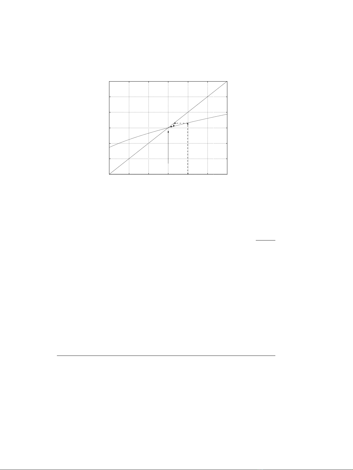
K(x)=sqrt(2x+3)
y=x
Fixed Point x*=3
x
K(x),y
Figure 7.1 FPI solution for roots of F(x)=x2
−2x−3
Tank 1985; Luh et al. 1998). The Lyapunov stability of neural networks is studied in
detail in Han et al. (1989) and Jin and Gupta (1996).
The concept of fixed point will be central to much of what follows, for which the
basic theorems and principles are introduced in Appendix G.
Point x∗is called a fixed point of a function Kif it satisfies K(x∗)=x∗, i.e. the
value x∗is unchanged under the application of function K. For instance, the roots of
function F(x)=x2−2x−3 can be found by rearranging xk+1 =K(xk)=√2xk+3
via fixed point iteration. The roots of the above function are −1 and 3. The FPI
which started from x0= 4 converges to within 10−5of the exact solution in nine
steps, which is depicted in Figure 7.1. This example is explained in more detail in
Appendix G.
One of the virtues of neural networks is their processing power, which rests upon
their ability to converge to a set of fixed points in the state space. Stability analysis,
therefore, is essential for the derivation of conditions that assure convergence to these
fixed points. Stability, although necessary, is not sufficient for effective processing
(see Appendix H), since in practical applications, it is desirable that a neural system
converges to only a preselected set of fixed points. In the remainder of this chapter,
two different aspects of equilibrium, i.e. the static aspect (existence and uniqueness
of equilibrium states) and the dynamic aspect (global stability, rate of convergence),
are studied. While analysing global asymptotic stability,2it is convenient to study the
static problem of the existence and uniqueness of the equilibrium point first, which is
the necessary condition for GAS.
2It is important to note that the iterates of random Lipschitz functions converge if the functions
are contracting on the average (Diaconis and Freedman 1999). The theory of random operators is
a probabilistic generalisation of operator theory. The study of probabilistic operator theory and its
applications was initiated by the Prague school under the direction of Antonin Spacek, in the 1950s
(Bharucha-Reid 1976). They recognised that it is necessary to take into consideration the fact that
the operators used to describe the behaviour of systems may not be known exactly. The application
of this theory in signal processing is still under consideration and can be used to analyse stochastic
learning algorithms (Chambers et al. 2000).

118 OVERVIEW
7.3 Overview
The role of the nonlinear activation function in the global asymptotic convergence of
recurrent neural networks is studied. For a fixed input and weights, a repeated appli-
cation of the nonlinear difference equation which defines the output of a recurrent
neural network is proven to be a relaxation, provided the activation function satis-
fies the conditions required for a contraction mapping. This relaxation is shown to
exhibit linear asymptotic convergence. Nesting of modular recurrent neural networks
is demonstrated to be a fixed point iteration in a spatial form.
7.4 A Fixed Point Interpretation of Convergence in Networks with a
Sigmoid Nonlinearity
To solve many problems in the field of optimisation, neural control and signal process-
ing, dynamic neural networks need to be designed to have only a unique equilibrium
point. The equilibrium point ought to be globally stable to avoid the risk of spuri-
ous responses or the problem of local minima. Global asymptotic stability (GAS) has
been analysed in the theory of both linear and nonlinear systems (Barnett and Storey
1970; Golub and Van Loan 1996; Haykin 1996a; Kailath 1980; LaSalle 1986; Priest-
ley 1991). For nonlinear systems, it is expected that convergence in the GAS sense
depends not only on the values of the parameter vector, but also on the parameters
of the nonlinear function involved. As systems based upon sigmoid functions exhibit
stability in the bounded input bounded output (BIBO) sense, due to the saturation
type sigmoid nonlinearity, we investigate the characteristics of the nonlinear activa-
tion function to obtain GAS for a general RNN-based nonlinear system. In that case,
both the external input vector to the system x(k) and the parameter vector w(k) are
assumed to be a time-invariant part of the system under fixed point iteration.
7.4.1 Some Properties of the Logistic Function
To derive the conditions which the nonlinear activation function of a neuron should
satisfy to enable convergence of real-time learning algorithms, activation functions
of a neuron are analysed in the framework of contraction mappings and fixed point
iteration.
Observation 7.4.1. The logistic function
Φ(x)= 1
1+e
−βx (7.4)
is a contraction on [a, b]∈Rfor 0<β<4and the iteration
xi+1 =Φ(xi) (7.5)
converges to a unique solution x∗from ∀x0∈[a, b]∈R.
Proof. By the contraction mapping theorem (CMT) (Appendix G), function Kis a
contraction on [a, b]∈Rif

STABILITY ISSUES IN RNN ARCHITECTURES 119
abK(a) K(b)
Figure 7.2 The contraction mapping
(i) x∈[a, b]⇒K(x)∈[a, b],
(ii) ∃γ<1∈R+s.t. |K(x)−K(y)|γ|x−y|∀x, y ∈[a, b].
The condition (i) is illustrated in Figure 7.2. The logistic function (7.4) is strictly
monotonically increasing, since its first derivative is strictly greater than zero. Hence,
in order to prove that Φis a contraction on [a, b]∈R, it is sufficient to prove that it
contracts the upper and lower bound of interval [a, b], i.e. aand b, which in turn gives
•a−Φ(a)0,
•b−Φ(b)0.
These conditions will be satisfied if the function Φis smaller in magnitude than the
curve y=x, i.e. if
|x|>
1
1+e
−βx ,β>0.(7.6)
Condition (ii) can be proven using the mean value theorem (MVT) (Luenberger 1969).
Namely, as the logistic function Φ(7.4) is differentiable, for ∀x, y ∈[a, b], ∃ξ∈(a, b)
such that
|Φ(x)−Φ(y)|=|Φ′(ξ)(x−y)|=|Φ′(ξ)||x−y|.(7.7)
The first derivative of the logistic function (7.4) is
Φ′(x)=1
1+e
−βx ′
=βe−βx
(1+e
−βx)2,(7.8)
which is strictly positive, and for which the maximum value is Φ′(0) = β/4. Hence,
for β4, the first derivative Φ′1. Finally, for γ<1⇔β<4, function Φgiven
in (7.4) is a contraction on [a, b]∈R.
Convergence of FPI: if x∗is a zero of x−Φ(x) = 0, or in other words the fixed
point of function Φ, then for γ<1(β<4)
|xi−x∗|=|Φ(xi−1)−Φ(x∗)|γ|xi−1−x∗|.(7.9)
Thus, since for γ<1⇒{γ}ii
−→ 0
|xi−x∗|γi|x0−x∗|⇒ lim
i→∞ xi=x∗(7.10)
and iteration xi+1 =Φ(xi) converges to some x∗∈[a, b].
Convergence/divergence of the FPI clearly depends on the size of slope βin Φ.
Considering the general nonlinear system Equation (7.2), this means that for a fixed
input vector to the iterative process and fixed weights of the network, an FPI solution
depends on the slope (first derivative) of the nonlinear activation function and some
measure of the weight vector. If the solution exists, that is the only value to which