14
THE LAPLACE TRANSIVRh4
Example 2.1. Find the
Laplace
transform of the function
f(t)
=
1
According to Eq. (2.
l),
f(s)
=
J-ow(l)e-“‘df
=
-
e-S’
t=cu
S
t=O
=
f
Thus,
L(1) =
f
There
am
several facts worth noting at this point:
1. The
Laplace
transform f(s) contains no information about the behavior of f(t)
for
t
< 0. This is not a limitation for control system study because
t
will
represent the time variable and we shall be interested in the behavior of systems
only for positive time. In fact, the variables and systems are usually defined so
that f (t) = 0 for
t
< 0. This will become clearer as we study specific examples.
2. Since the
Laplace
transform is defined in Eq. (2.1) by an improper integral,
it will not exist for every function f(t). A rigorous definition of the class of
functions possessing
Laplace
transforms is beyond the scope of this book, but
readers will note that every function of interest to us does satisfy the requirements
for possession of a transform.*
3. The
Laplace
transform is linear. In mathematical notation,
this
means:
~bfl(~)
+
bf2Wl
=
4fl(O)
+
mf2Wl
where a and b are constants, and f
1
and
f2
am
two functions of
t.
Proof. Using the definition,
Uafl(t)
+
bfdt))
=
lom[aflO)
+
bf2(~)le-s’d~
=a
I
omfl(r)e-stdt +
blom
f2(t)e-S’dr
=
&flW )
+
bUM )l
4. The
Laplace
transform operator transforms a function of the variable
I
to a func-
tion of the variable s. The
I
variable is eliminated by
the
integration.
Tkansforms
of Simple Fhnctions
We now proceed to derive the transforms of some simple and useful functions.
*For details on this and related mathematical topics, see Churchill (1972).
THE
LAPLACE
TRANSFORM
15
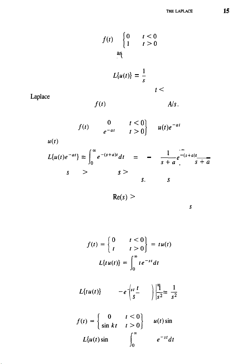
1. The step function
.m
= i
y
t<O
t>O
This important function is known a$ the unit-step function and will henceforth
be denoted by u(t). From Example 2.1, it is clear that
L{u(t)}
=
f
As expected, the behavior of the function for
t
< 0 has no effect on its
Laplace
transform. Note that as a consequence of linearity, the transform of
any constant A, that is,
f(t)
= Au(t), is just f(s) = A/s.
2. The exponential function
f (t )
=
._“,,
I
t <O
t >O
I
=
u(t )e-“’
where u(t) is the unit-step function. Again proceeding according to definition,
I
m m
L{u(t )e en’}
=
1
0
e-(s+a )rdt
=
_
Ae-(s+a )t
-
0
S+U
provided that
s
+ a > 0, that is, s > -a. In this case, the convergence of
the integral depends on a suitable choice of
S.
In case s is a complex number,
it may be shown that this condition becomes
Re(s) > -a
For problems of interest to us it will always be possible to choose
s
so that these
conditions are satisfied, and the reader uninterested in mathematical niceties
can ignore this point.
3. The ramp function
Integration by parts yields
L{ t u(t )}
=
-eesf
f .
+
f
i
ii
cc
s0
=
f
4. The sine function
= u(t)sin kt
L{u(t)sin kt} = sin kt ems’dt
16
THE
LAPLACE
TRANsmRM
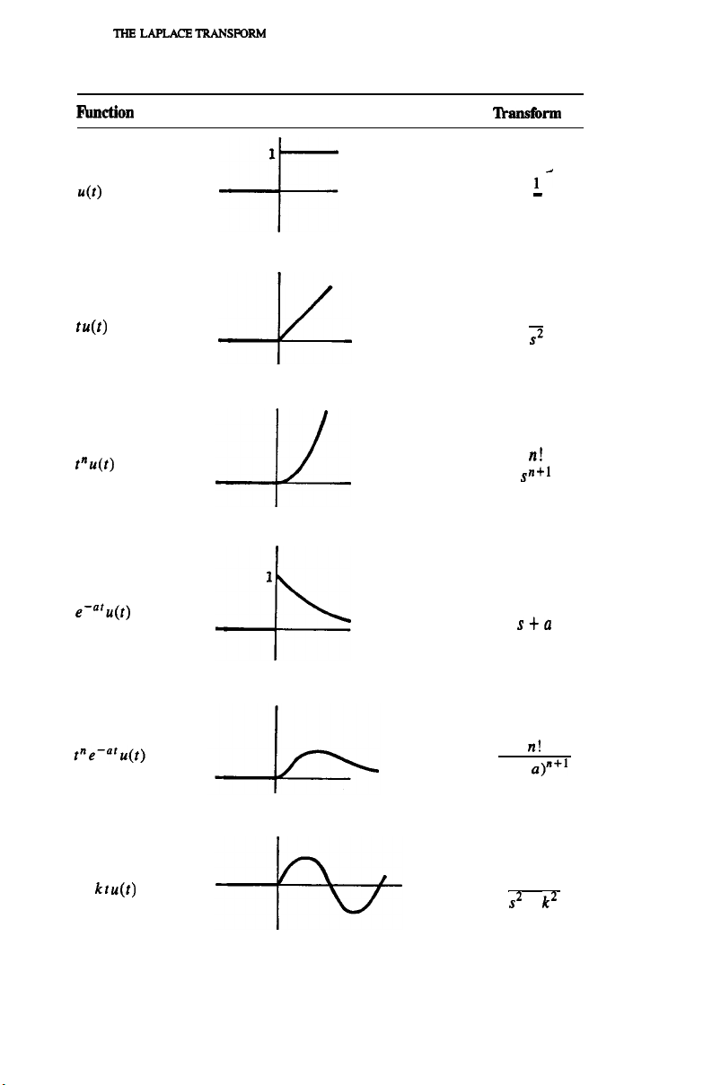
TABLE 2.1
FilDCtiOIl
Graph ‘llxmfbrm
1
u(t)
-F
ld
-
S
W)
Pu(t)
e-= “u(t)
sin kt u(t)
-4
4
1
4
1
7
?I!
sn+l
1
s+a
n!
(s + a)“+l
k
s2 +
k2
THE LAPLACE TRANSFORM
17
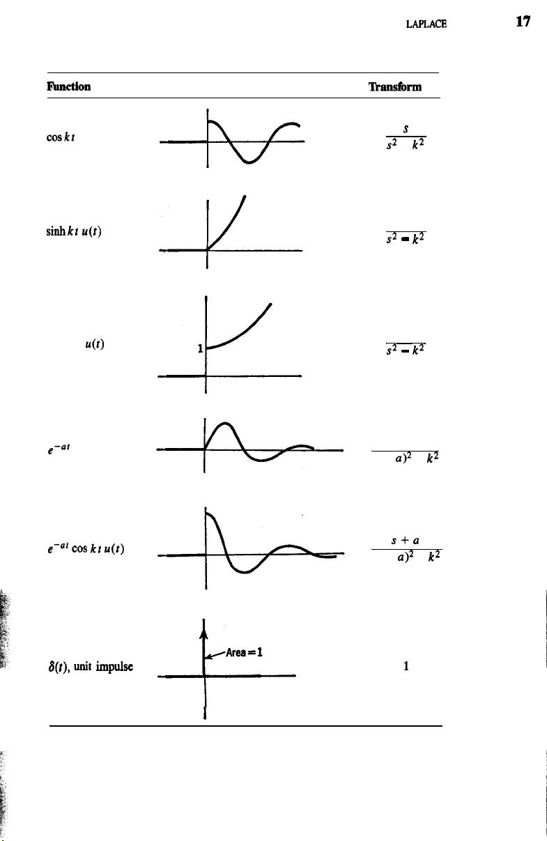
TABLE 2.1 (Continued)
lhlCtiOll
Graph
l.hmshm
coskt u(t)
sinhkt
u(t)
coshkr u(r)
e-= ’ Sink? u(r)
e-
cos
kt
u(t)
*
S(f),
unit
impulse
-k-
1
Area
=
1
+-
s
s2 +
k2
k
s2
-
k2
S
s2
-
k2
k
(s + a)? +
k2
s+a
(s +
a)2
+
k2
1
I
18
THE LAPLACE TRANSFORM
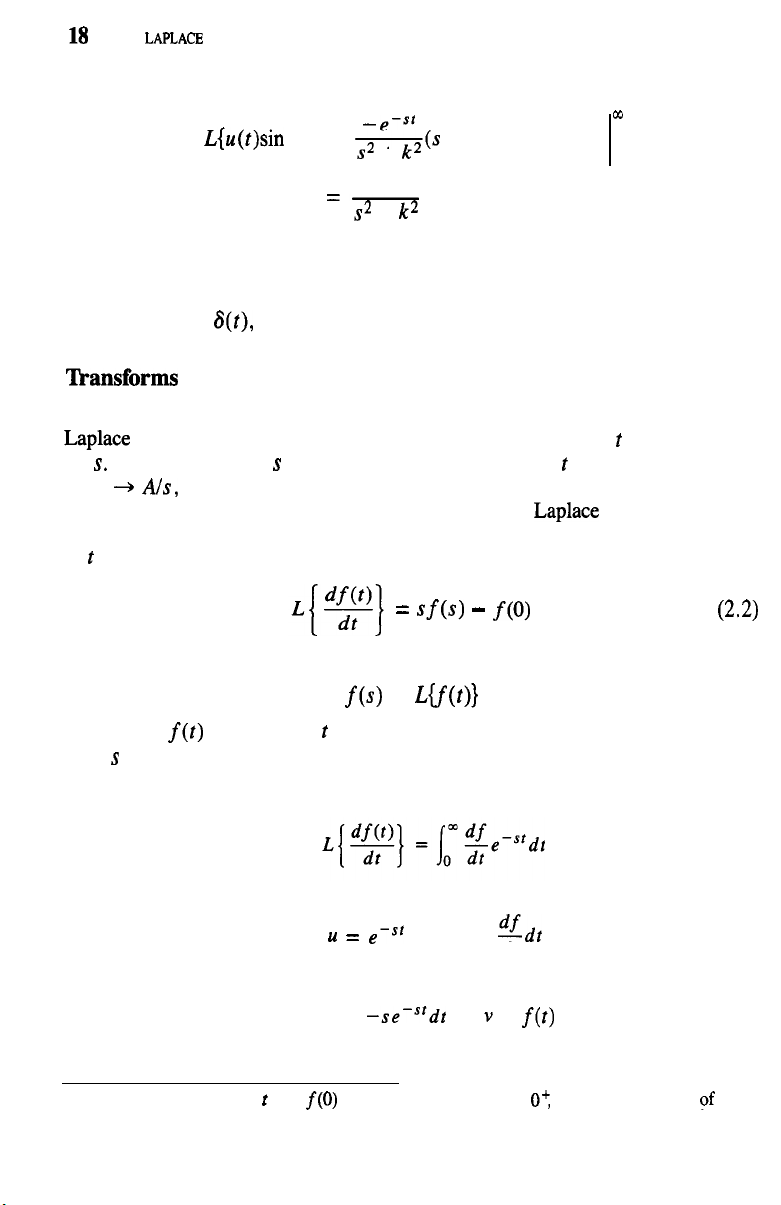
Integrating by parts,
L{u(t)sin
-e-St
01
kt} =
-(s
sin kt + k cos kt)
s* +
k*
0
k
=-
s* +
k*
In a like manner, the transforms of other simple functions may be derived.
Table 2.1 is a summary of transforms that will be of use to us. Those which have
not been derived here can be easily established by direct integration, except for
the transform of 6(t), which will be discussed in detail in Chap. 4.
Transforms of Derivatives
At this point, the reader may wonder what has been gained by introduction of the
Laplace
transform. The transform merely changes a function of
t
into a function
of
S.
The functions of s look no simpler than those of
t
and, as in the case
of A
--,
A/s, may actually be more complex. In the next few paragraphs, the
motivation will become clear. It will be shown that the
Laplace
transform has the
remarkable property of transforming the operation of differentiation with respect
to
t
to that of multiplication by s. Thus, we claim that
=
sf(s)
-
f(O)
(2.2)
where
f(s) = u.f(t)1
and f(0) is
f(t)
evaluated at
t
= 0. [It is essential not to interpret f(0) as f(s)
with s = 0. This will be clear from the following proof.]*
Proof.
To
integrate this
by parts, let
u
= e-S’ dv =
dfdt
dt
Then
du = --sems’dt
v
=
f(t)
* If f(t) is discontinuous at
t
= 0, f(0) should he evaluated at t =
O’,
i.e., just to the right
of
the
origin. Since we shall seldom want to differentiate functions that are discontinuous at the origin, this
detail is not of great importance. However, the reader is cautioned to watch carefully for situations
in which such discontinuities occur.


%20--%3e%3cdefs%3e%3cstyle%3e%20.st0%20{%20fill:%20%23fff;%20}%20.st1%20{%20fill:%20%237800fa;%20}%20%3c/style%3e%3c/defs%3e%3cpath%20class='st1'%20d='M117.78,12.18H43.11c2.9,3.47,4.65,7.94,4.65,12.82,0,5.6-2.3,10.66-6.01,14.29h76.02l7.22-13.56-7.22-13.56Z'/%3e%3cg%3e%3cpath%20class='st0'%20d='M53.58,26.17h-.59v-1.46h.59v-4.96h2.83c1.78,0,2.67.94,2.67,2.82v5.76c0,1.87-.89,2.81-2.67,2.81h-2.83v-4.96ZM55.36,21.37v3.34h1.1v1.46h-1.1v3.34h1.01c.61,0,.91-.37.91-1.1v-5.93c0-.74-.3-1.1-.91-1.1h-1.01Z'/%3e%3cpath%20class='st0'%20d='M65.99,31.14h-1.8l-.31-2.07h-2.19l-.31,2.07h-1.64l1.82-11.39h2.62l1.82,11.39ZM65.28,18.04c-.25.46-.51.77-.75.94-.21.15-.47.22-.79.22-.26,0-.57-.07-.92-.22l-.38-.15c-.14-.05-.26-.07-.37-.07-.3,0-.53.18-.71.54l-.91-.68c.25-.46.51-.77.75-.94.21-.14.48-.21.79-.21.26,0,.57.07.92.21l.38.15c.14.05.26.07.37.07.3,0,.53-.18.71-.54l.91.68ZM61.91,27.52h1.73l-.87-5.76-.87,5.76Z'/%3e%3cpath%20class='st0'%20d='M74.53,26.89v1.52c0,1.91-.89,2.86-2.67,2.86s-2.67-.95-2.67-2.86v-5.93c0-1.91.89-2.86,2.67-2.86s2.67.95,2.67,2.86v1.11h-1.69v-1.22c0-.75-.31-1.12-.93-1.12s-.93.37-.93,1.12v6.15c0,.74.31,1.11.93,1.11s.93-.37.93-1.11v-1.63h1.69Z'/%3e%3cpath%20class='st0'%20d='M81.4,31.14h-1.8l-.31-2.07h-2.19l-.31,2.07h-1.64l1.82-11.39h2.62l1.82,11.39ZM75.9,19.2l1.52-1.91h1.71l1.51,1.91h-1.61l-.76-.95-.75.95h-1.61ZM77.32,27.52h1.73l-.87-5.76-.87,5.76ZM83.1,15.99l-1.76,1.91h-1.26l1.17-1.91h1.86Z'/%3e%3cpath%20class='st0'%20d='M84.86,19.75c1.78,0,2.67.94,2.67,2.82v1.48c0,1.87-.89,2.81-2.67,2.81h-.85v4.28h-1.79v-11.39h2.64ZM84.01,21.37v3.86h.85c.58,0,.87-.36.87-1.08v-1.71c0-.71-.29-1.07-.87-1.07h-.85Z'/%3e%3cpath%20class='st0'%20d='M93.51,19.75c1.78,0,2.67.94,2.67,2.82v1.48c0,1.87-.89,2.81-2.67,2.81h-.85v4.28h-1.79v-11.39h2.64ZM92.66,21.37v3.86h.85c.58,0,.87-.36.87-1.08v-1.71c0-.71-.29-1.07-.87-1.07h-.85Z'/%3e%3cpath%20class='st0'%20d='M98.8,31.14h-1.79v-11.39h1.79v4.88h2.03v-4.88h1.83v11.39h-1.83v-4.88h-2.03v4.88Z'/%3e%3cpath%20class='st0'%20d='M105.36,24.55h2.46v1.62h-2.46v3.34h3.09v1.63h-4.88v-11.39h4.88v1.63h-3.09v3.18ZM108.17,17.29l-1.76,1.91h-1.26l1.17-1.91h1.86Z'/%3e%3cpath%20class='st0'%20d='M112.2,19.75c1.78,0,2.67.94,2.67,2.82v1.48c0,1.87-.89,2.81-2.67,2.81h-.85v4.28h-1.79v-11.39h2.64ZM111.35,21.37v3.86h.85c.58,0,.87-.36.87-1.08v-1.71c0-.71-.29-1.07-.87-1.07h-.85Z'/%3e%3c/g%3e%3ccircle%20class='st1'%20cx='25'%20cy='25'%20r='20'/%3e%3cpath%20class='st0'%20d='M32.78,19.27c2.92,0,4.43,2.55,5.28,5.33l.71,2.17c.14.38-.33.75-.71.75h-5.61c.19-.33.24-.71.09-1.08l-.75-2.45c-.43-1.32-.99-2.64-1.79-3.77.75-.57,1.65-.94,2.78-.94h0ZM25,18.38c3.25,0,4.9,2.78,5.89,5.89l.76,2.45c.14.42-.33.8-.8.8h-11.69c-.42,0-.94-.38-.8-.8l.75-2.45c.99-3.11,2.64-5.89,5.89-5.89h0ZM25,11.35c1.74,0,3.11,1.37,3.11,3.11s-1.37,3.11-3.11,3.11-3.11-1.41-3.11-3.11,1.41-3.11,3.11-3.11h0ZM17.27,19.27c1.08,0,1.98.38,2.73.94-.8,1.13-1.37,2.45-1.74,3.77l-.8,2.45c-.14.38-.05.75.09,1.08h-5.56c-.42,0-.9-.38-.75-.75l.71-2.17c.9-2.78,2.41-5.33,5.33-5.33h0ZM17.27,12.91c1.51,0,2.78,1.27,2.78,2.83s-1.27,2.83-2.78,2.83-2.83-1.27-2.83-2.83,1.27-2.83,2.83-2.83h0ZM32.78,12.91c1.56,0,2.78,1.27,2.78,2.83s-1.23,2.83-2.78,2.83-2.83-1.27-2.83-2.83,1.27-2.83,2.83-2.83h0ZM27.07,28.56v.09c0,.57-.24,1.08-.61,1.46h0v.05c-.38.33-.9.57-1.46.57s-1.08-.24-1.46-.61h0c-.38-.38-.61-.9-.61-1.46v-.09h1.41v.09c0,.19.05.38.19.47v.05c.09.09.28.19.47.19s.38-.09.47-.19v-.05c.14-.09.24-.28.24-.47t-.05-.09h1.41ZM30.99,28.56v.09c0,1.65-.66,3.16-1.74,4.24-1.08,1.08-2.59,1.79-4.24,1.79s-3.16-.71-4.24-1.79l-.05-.05c-1.04-1.08-1.7-2.55-1.7-4.2v-.09h1.41v.09c0,1.27.47,2.4,1.27,3.25h.05c.85.85,1.98,1.37,3.25,1.37s2.4-.52,3.25-1.37c.85-.8,1.37-1.98,1.37-3.25v-.09h1.37ZM34.99,28.56v.09c0,2.78-1.13,5.28-2.92,7.07-1.79,1.79-4.29,2.92-7.07,2.92s-5.23-1.13-7.07-2.92c-1.79-1.79-2.92-4.29-2.92-7.07v-.09h1.41v.09c0,2.4.94,4.53,2.5,6.08,1.56,1.56,3.72,2.5,6.08,2.5s4.52-.94,6.08-2.5c1.56-1.56,2.5-3.68,2.5-6.08v-.09h1.41Z'/%3e%3c/svg%3e)