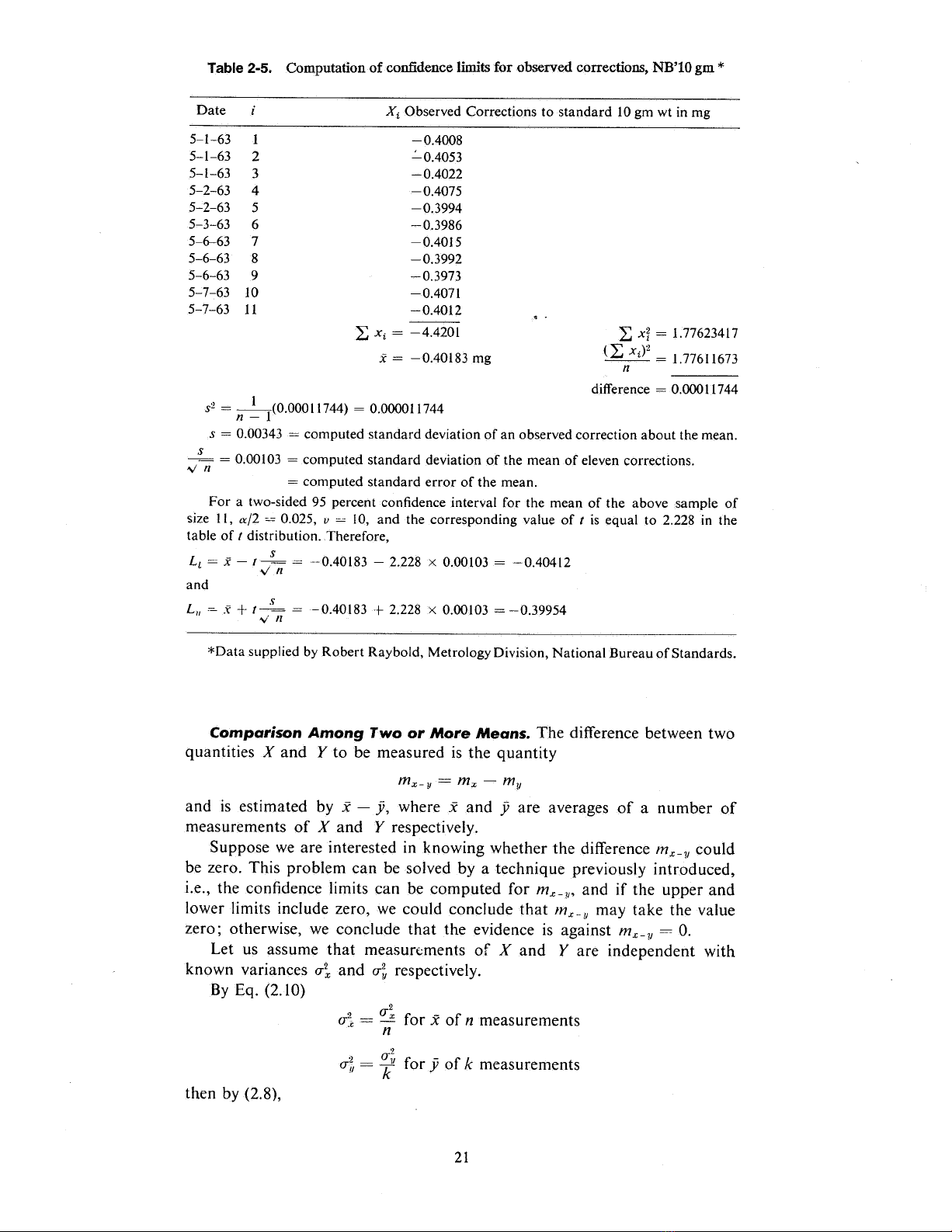
Table 2-5. Computation of confidence limits for ob:;erved corrections, NB' lO gm "'
Date Xi Observed Corrections to standard 10 gm wt in mg
63
63 2
63
63 4
63
63 6
6-63 7
63
63
63
63
0.4008
~0.4053
~0.4022
4075
0.3994
0.3986
0.4015
3992
3973
0.4071
0.4012
Xi
= -
4.4201
= -
0.40183 mg
xI = 1.77623417
(~
= 1.77611673
2 = (0,00011744) = 0,000011744
S = 0,00343 = computed standard deviation of an observed correction about the mean.
= 0.00103 = computed standard deviation of the mean of eleven corrections.
= computed standard error of the mean,
For a two-sided 95 percentcon.fidenceinterval for the mean of the above sample of
size 11 a/2 = 0.025, 10, and the corresponding value of is equal to 2,228 in the
table of distribution. Therefore
Ll
= --
0.40183 - 2.228 x 0,00103 = - 0.40412
and
lI
= .
X' +
= -
0.40183 + 2,228 x 0.00103 = - 39954
difference = 0.00011744
*Data supplied by Robert Raybold, Metrology Division, National Bureau of Standards.
Comparison Among Two or More Means. The difference between two
quantities and to be measured is the quantity
mx_ mx
and is estimated by :X
y,
where and yare averages of a number of
measurements of and respectively.
Suppose we are interested in knowing whether the difference mx- could
be zero. This problem can be solved by a technique previously introduced,
, the confidence limits can be computed for mx_
y,
and if the upper and
lower limits include zero, we could conclude that mx_ may take the value
zero; otherwise , we conclude that the evidence is against mx-
Let us assume that measur(;ments of and Yare independent with
known variances ()~ and (); respectively.
By Eq. (2. 10)
2 = ,2. for of measurements
()~()j,
for of measurements
then by (2. 8),
Simpo PDF Merge and Split Unregistered Version - http://www.simpopdf.com
2. - u;, U y
Therefore, the quantity
(x
y)
- 0
J:~
is approximately normally distributed with mean zero and a standard
deviation of one under the assumption mx-
If Ux and are not known, but the two can be assumed to be approxi-
mately equal, e. and yare measured by the same process, then s~ and
s~ can be pooled by Eq. (2- 15), or
(n l)s~ (k l)s~
.~ 2
, '
(2- 17)
This pooled computed variance estimates
u~
so that
2.
Thus, the quantity
(x
y)
- 0
In ;tk k
is distributed as Student's " , and a confidence interval .can be set about
mx-y with - 2 and I-a. If this interval does not include
zero, we may conclude that the evidence is strongly against the hypothesis
(2- 18)
mx
As an example, we continue with the calibration of weights with
NB' lO gm. For II subsequent observed corrections during September and
October, the confidence interval (computed in the same manner as in the
preceding example) has been found to be
Ll
= -
0.40782
Lu 0.40126
Also
y = -
0.40454 and
'"Jk
00147
It is desired to compare the means of observed corrections for the two sets
of data. Here
0.40183
s~ = 0.000011669
= -
40454
s~ = 0.000023813
s~ -!(0.000035482) = 0.000017741
n+k 11+11
---rik 121 =
In ---rik . TI X 0. 000017741 = 0.00180
Simpo PDF Merge and Split Unregistered Version - http://www.simpopdf.com
For al2 = 0.025 , 1 ~ = 0. , and 086. Therefore
(x ji)
-/n ;tk k 00271 + 2.086 x 0.00180
= 0.00646
Lt (x ji) -/n
;tk k 001O4
Since Ll ~ 0 ~ Lu shows that the confidence interval includes zero, we
conclude that there is no evidence against the hypothesis that the two
observed average corrections are the same, or mx
y.
Note, however
that we would reach a conclusion of no difference wherever the magnitude
of ~ ji (0.00271 mg) is less than the half-width of the confidence interval
(2.086 X 0.00180 = 0.00375 mg) calculated for the particular case. When
the true difference mx- is large, the above situation is not likely to happen;
but when the true difference is small, say about 0.003 mg, then it is highly
probable that a concl usion of no difference will still be reached. If a detection
of difference of this magnitude is of interest, more measurements will
be needed.
The following additional topics are treated in reference 4.
l. Sample sizes required under certain specified conditions-Tables
and
2. ()~ cannot be assumed to be equal to ()~-Section 3-
3. Comparison of several means by Studentized range-Sections 3-
and 15-
Comparison of variances or ranges. As we have seen, the precision of
a measurement process can be expressed in terms of the computed standard
deviation, the variance, or the range. To compare the precision of two
processes and any of the three measures can be used , depending on
the preference and convenience of the user.
Let s~ be the estimate of ()~ with Va degrees of freedom, and s~ be the
estimate of (J"~ with Vb degrees of freedom. The ratio s~/s~ has a distri-
bution depending on Va and Vb' Tables of upper percentage points of
are given in most statistical textbooks, e. , reference 4, Table and
Section 4-
In the comparison of means , we were interested in finding out if the
absolute difference between and mb could reasonably be zero; similarly,
here we may be interested in whether
()~
()~, or
()~/()~
1. In practice
however, we are usually concerned with whether the imprecision of one
process exceeds that of another process. We could, therefore, compute the
ratio of s~ to s~, and the question arises: If in fact
()~ =
()~, what is the
probability of getting a value of the ratio as large as the one observed?
For each pair of values of and Vb, the tables list the values of which are
exceeded with probability the upper percentage point of the distribution
of F. If the computed value of exceeds this tabulated value of
then we conclude that the evidence is against the hypothesis
()~ =
()~; if it
is less, we conclude that ()~ could be eql!al to
()~.
For example, we could compute the ratio of s~ to s~ in the preceding
two examples.
Here the degrees of freedom Vx = 10, the tabulated value of
which is exceeded 5 percent of the time for these degrees of freedom is
, and
000023813 - 2041
s~ - 0.000011669
Simpo PDF Merge and Split Unregistered Version - http://www.simpopdf.com
Since 2.04 is less than 2. , we conclude that there is no reason to believe
that the precision of the calibration process in September and October is
poorer than that of May.
For small degrees of freedom , the critical value of is rather large
, for Vb = 3, and = 0.05, the value of is 9. 28. It follows
that a small difference between O"~ and O"E is not likely to be detected with a
small number of measurements from each process. The table below gives
the approximate number of measurements required to have a four-out-
of-five chance of detecting whether is the indicated multiple of (Tb (while
maintaining at 0.05 the probability of incorrectly concluding that O"b,
when in fact O"b
Multiple
1.5
No. of measurements
Table A- II in reference 4 gives the critical values of the ratios of ranges
and Tables A-20 and A-21 give confidence limits on the standard deviation
of the process based on computed standard deviation.
Cont.rol Charts Technique for
Maintaining .Stability and Precision
A laboratory which performs routine measurement or calibration opera-
tions yields , as its daily product, numbers-averages, standard deviations
and ranges. The control chart techniques therefore could be applied to these
numbers as products of a manufacturing process to furnish graphical
evidence on whether the measurement process is in statistical control or out
of statistical control. If it is out of control, these charts usually also indicate
where and when the trouble occurred.
Control Chart for Averages, The basic concept of a control chart is
in accord with what has been disctlssed thus far. A measurement process
with limiting mean and standard deviation (J is assumed. The sequence
of numbers produced is divided into "rational" subgroups, e. , by day,
by a set of calibrations, etc. The averages of these subgroups are computed.
These averages will have a mean and a standard deviation 0"/ vn where
is the number of measurements within each subgroup. These averages
are approximately normally distributed.
In the construction of the control chart for averages is plotted as the
center line k(O"/vn) and k(O"/vn) are plotted as control limits,
and the averages are plotted in an orderly sequence. If is taken to be 3
we know that the chance of a plotted point falling outside of the limits
if the process is in control, is very small. Therefore, if a plotted point falls
outside these limits, a warning is sounded and investigative action to locate
the "assignable" cause that produced the departure, or corrective measures
are called for.
The above reasoning would be applicable to actual cases only if we have
chosen the proper standard deviation (T. If the standard deviation is estimated
by pooling the estimates computed from each subgroup and denoted by 0" w
(within group), obviously differences , if any, between group averages have
Simpo PDF Merge and Split Unregistered Version - http://www.simpopdf.com
not been taken into consideration. Where there are between-group differences
the variance of the individual is not u;,/n but, as we have seen before
u~ (u;,/n), where u~ represents the variance due to differences between
groups. If u~ is of any consequence as compared to u;" many of the values
would exceed the limits constructed by using alone.
Two alternatives are open to us: (l) remove the cause of the between-
group variation; or, (2) if such variation is a proper component of error
take it into account as has been previously discussed.
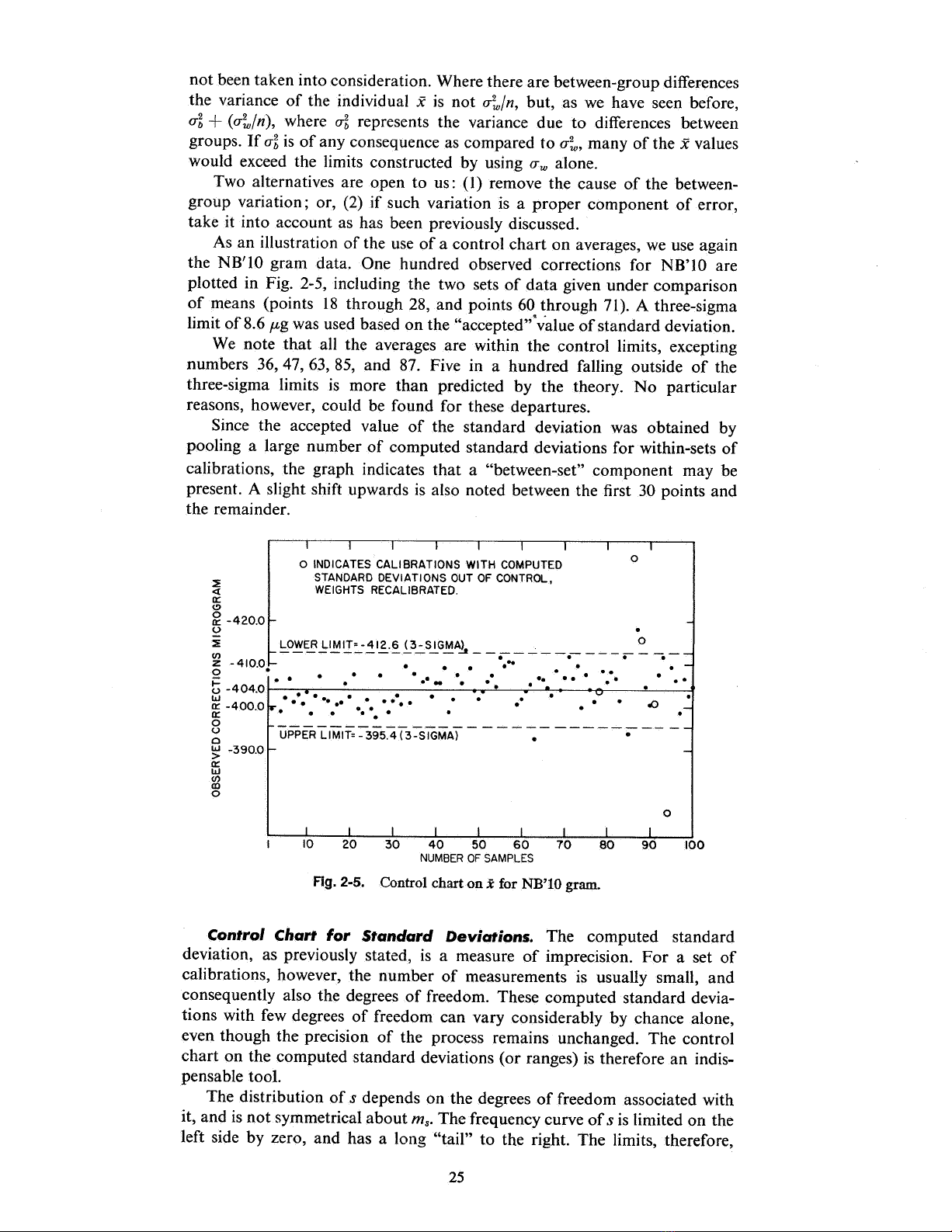
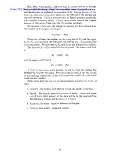
As an illustration of the use of a control chart on averages, we use again
the NB' lO gram data. One hundred observed corrections for NB' lO are
plotted in Fig. 2- , including the two sets of data given under comparison
of means (points 18 through 28 , and points 60 through 71). A three-sigma
limit of 8. 6 p,g was used based on the "accepted" valueof standard deviation.
We note that all the averages are within the control limits, excepting
numbers 36, 47, 63 , 85, and 87. Five in a hundred falling outside of the
three-sigma limits is more than predicted by the theory. No particular
reasons, however, could be found for these departures.
Since the accepted value of the standard deviation was obtained
pooling a large number of computed standard deviations for within-sets of
calibrations, the graph indicates that a "between-set" component may be
present. A slight shift upwards is also noted between the first 30 points and
the remainder.
:::;:
c:(
a::
:E - 20.
:::;:
LOWER lIMIT=- 412. 6 (3- SIGMA)
------------ ~------------- --
~ - 410,0 .
. . . .
0 o o.
i=
. . .. .
0 0
. .
. 0
u -404, . . o
. . . . ~ -
400.
. .~ -
390,
a::
CJ)
0 INDICATES CALIBRATIONS WITH COMPUTED
STANDARD DEVIATIONS OUT OF CONTROl,
WEIGHTS RECALIBRATED.
---------- ----- ----- --~------
UPPER LlMIT=- 395.4(3- SIGMA)
100
FIg. 2-5. Control chart on j for NB' 10 gram.
Control ChQrt lor StQndQrd f)ev;(Jf;ons. The computed standard
deviation, as previously stated, is a measure of imprecision. For a set of
calibrations, however, the number of measurements is usually small, and
consequently also the degrees of freedom. These computed standard devia-
tions with few degrees of freedom can vary considerably by chance alone
even though the precision of the process remains unchanged. The control
chart on the computed standard deviations (or ranges) is therefore an indis-
pensable tool.
The distribution of depends on the degrees of freedom associated with
, and is not symmetrical about mo. The frequency curve of is limited on the
left side by zero, and has a long "tail" to the right. The limits, therefore
Simpo PDF Merge and Split Unregistered Version - http://www.simpopdf.com
![Bảng tra dung sai lắp ghép Lê Hoàng Lâm: [Thêm từ mô tả phù hợp]](https://cdn.tailieu.vn/images/document/thumbnail/2022/20221205/camtucau205/135x160/9731670233749.jpg)


![Cẩm nang Gia công kim loại Việt Nam [mới nhất]](https://cdn.tailieu.vn/images/document/thumbnail/2026/20260513/baobinh_011/135x160/7971778670576.jpg)


![Giáo trình Hàn ống nâng cao (Nghề Hàn - CĐ) Trường Cao đẳng nghề Hải Dương [Mới nhất]](https://cdn.tailieu.vn/images/document/thumbnail/2025/20251212/laphong0906/135x160/47521779076565.jpg)


%20--%3e%3cdefs%3e%3cstyle%3e%20.st0%20{%20fill:%20%23fff;%20}%20.st1%20{%20fill:%20%237800fa;%20}%20%3c/style%3e%3c/defs%3e%3cpath%20class='st1'%20d='M117.78,12.18H43.11c2.9,3.47,4.65,7.94,4.65,12.82,0,5.6-2.3,10.66-6.01,14.29h76.02l7.22-13.56-7.22-13.56Z'/%3e%3cg%3e%3cpath%20class='st0'%20d='M53.58,26.17h-.59v-1.46h.59v-4.96h2.83c1.78,0,2.67.94,2.67,2.82v5.76c0,1.87-.89,2.81-2.67,2.81h-2.83v-4.96ZM55.36,21.37v3.34h1.1v1.46h-1.1v3.34h1.01c.61,0,.91-.37.91-1.1v-5.93c0-.74-.3-1.1-.91-1.1h-1.01Z'/%3e%3cpath%20class='st0'%20d='M65.99,31.14h-1.8l-.31-2.07h-2.19l-.31,2.07h-1.64l1.82-11.39h2.62l1.82,11.39ZM65.28,18.04c-.25.46-.51.77-.75.94-.21.15-.47.22-.79.22-.26,0-.57-.07-.92-.22l-.38-.15c-.14-.05-.26-.07-.37-.07-.3,0-.53.18-.71.54l-.91-.68c.25-.46.51-.77.75-.94.21-.14.48-.21.79-.21.26,0,.57.07.92.21l.38.15c.14.05.26.07.37.07.3,0,.53-.18.71-.54l.91.68ZM61.91,27.52h1.73l-.87-5.76-.87,5.76Z'/%3e%3cpath%20class='st0'%20d='M74.53,26.89v1.52c0,1.91-.89,2.86-2.67,2.86s-2.67-.95-2.67-2.86v-5.93c0-1.91.89-2.86,2.67-2.86s2.67.95,2.67,2.86v1.11h-1.69v-1.22c0-.75-.31-1.12-.93-1.12s-.93.37-.93,1.12v6.15c0,.74.31,1.11.93,1.11s.93-.37.93-1.11v-1.63h1.69Z'/%3e%3cpath%20class='st0'%20d='M81.4,31.14h-1.8l-.31-2.07h-2.19l-.31,2.07h-1.64l1.82-11.39h2.62l1.82,11.39ZM75.9,19.2l1.52-1.91h1.71l1.51,1.91h-1.61l-.76-.95-.75.95h-1.61ZM77.32,27.52h1.73l-.87-5.76-.87,5.76ZM83.1,15.99l-1.76,1.91h-1.26l1.17-1.91h1.86Z'/%3e%3cpath%20class='st0'%20d='M84.86,19.75c1.78,0,2.67.94,2.67,2.82v1.48c0,1.87-.89,2.81-2.67,2.81h-.85v4.28h-1.79v-11.39h2.64ZM84.01,21.37v3.86h.85c.58,0,.87-.36.87-1.08v-1.71c0-.71-.29-1.07-.87-1.07h-.85Z'/%3e%3cpath%20class='st0'%20d='M93.51,19.75c1.78,0,2.67.94,2.67,2.82v1.48c0,1.87-.89,2.81-2.67,2.81h-.85v4.28h-1.79v-11.39h2.64ZM92.66,21.37v3.86h.85c.58,0,.87-.36.87-1.08v-1.71c0-.71-.29-1.07-.87-1.07h-.85Z'/%3e%3cpath%20class='st0'%20d='M98.8,31.14h-1.79v-11.39h1.79v4.88h2.03v-4.88h1.83v11.39h-1.83v-4.88h-2.03v4.88Z'/%3e%3cpath%20class='st0'%20d='M105.36,24.55h2.46v1.62h-2.46v3.34h3.09v1.63h-4.88v-11.39h4.88v1.63h-3.09v3.18ZM108.17,17.29l-1.76,1.91h-1.26l1.17-1.91h1.86Z'/%3e%3cpath%20class='st0'%20d='M112.2,19.75c1.78,0,2.67.94,2.67,2.82v1.48c0,1.87-.89,2.81-2.67,2.81h-.85v4.28h-1.79v-11.39h2.64ZM111.35,21.37v3.86h.85c.58,0,.87-.36.87-1.08v-1.71c0-.71-.29-1.07-.87-1.07h-.85Z'/%3e%3c/g%3e%3ccircle%20class='st1'%20cx='25'%20cy='25'%20r='20'/%3e%3cpath%20class='st0'%20d='M32.78,19.27c2.92,0,4.43,2.55,5.28,5.33l.71,2.17c.14.38-.33.75-.71.75h-5.61c.19-.33.24-.71.09-1.08l-.75-2.45c-.43-1.32-.99-2.64-1.79-3.77.75-.57,1.65-.94,2.78-.94h0ZM25,18.38c3.25,0,4.9,2.78,5.89,5.89l.76,2.45c.14.42-.33.8-.8.8h-11.69c-.42,0-.94-.38-.8-.8l.75-2.45c.99-3.11,2.64-5.89,5.89-5.89h0ZM25,11.35c1.74,0,3.11,1.37,3.11,3.11s-1.37,3.11-3.11,3.11-3.11-1.41-3.11-3.11,1.41-3.11,3.11-3.11h0ZM17.27,19.27c1.08,0,1.98.38,2.73.94-.8,1.13-1.37,2.45-1.74,3.77l-.8,2.45c-.14.38-.05.75.09,1.08h-5.56c-.42,0-.9-.38-.75-.75l.71-2.17c.9-2.78,2.41-5.33,5.33-5.33h0ZM17.27,12.91c1.51,0,2.78,1.27,2.78,2.83s-1.27,2.83-2.78,2.83-2.83-1.27-2.83-2.83,1.27-2.83,2.83-2.83h0ZM32.78,12.91c1.56,0,2.78,1.27,2.78,2.83s-1.23,2.83-2.78,2.83-2.83-1.27-2.83-2.83,1.27-2.83,2.83-2.83h0ZM27.07,28.56v.09c0,.57-.24,1.08-.61,1.46h0v.05c-.38.33-.9.57-1.46.57s-1.08-.24-1.46-.61h0c-.38-.38-.61-.9-.61-1.46v-.09h1.41v.09c0,.19.05.38.19.47v.05c.09.09.28.19.47.19s.38-.09.47-.19v-.05c.14-.09.24-.28.24-.47t-.05-.09h1.41ZM30.99,28.56v.09c0,1.65-.66,3.16-1.74,4.24-1.08,1.08-2.59,1.79-4.24,1.79s-3.16-.71-4.24-1.79l-.05-.05c-1.04-1.08-1.7-2.55-1.7-4.2v-.09h1.41v.09c0,1.27.47,2.4,1.27,3.25h.05c.85.85,1.98,1.37,3.25,1.37s2.4-.52,3.25-1.37c.85-.8,1.37-1.98,1.37-3.25v-.09h1.37ZM34.99,28.56v.09c0,2.78-1.13,5.28-2.92,7.07-1.79,1.79-4.29,2.92-7.07,2.92s-5.23-1.13-7.07-2.92c-1.79-1.79-2.92-4.29-2.92-7.07v-.09h1.41v.09c0,2.4.94,4.53,2.5,6.08,1.56,1.56,3.72,2.5,6.08,2.5s4.52-.94,6.08-2.5c1.56-1.56,2.5-3.68,2.5-6.08v-.09h1.41Z'/%3e%3c/svg%3e)